


Abstract
We have obtained Infrared Telescope Facility/SpeX spectra of eight moderate-redshift (z = 0.7–2.4), radio-selected (log R* ≈ 0.4–1.9) broad absorption line (BAL) quasars. The spectra cover the rest-frame optical band. We compare the optical properties of these quasars to those of canonically radio-quiet (log R* ≲ 1) BAL quasars at similar redshifts and to low-redshift quasars from the Palomar–Green catalogue. As with previous studies of BAL quasars, we find that [O iii] λ5007 is weak, and optical Fe ii emission is strong, a rare combination in canonically radio-loud (log R* ≳ 1) quasars. With our measurements of the optical properties, particularly the Balmer emission-line widths and the continuum luminosity, we have used empirical scaling relations to estimate black hole masses and Eddington ratios. These lie in the range (0.4–2.6) × 109 M⊙ and 0.1–0.9, respectively. Despite their comparatively extreme radio properties relative to most BAL quasars, their optical properties are quite consistent with those of radio-quiet BAL quasars and dissimilar to those of radio-loud non-BAL quasars. While BAL quasars generally appear to have low values of [O iii] λ5007/Fe ii an extreme of ‘Eigenvector 1’, the Balmer line widths and Eddington ratios do not appear to significantly differ from those of unabsorbed quasars at similar redshifts and luminosities.
1 INTRODUCTION
In the past decade or so, a new class of AGN – radio-selected, broad absorption line (BAL) quasars – has brought new insights into the structure of quasars and quasar outflows. The deep images of the Faint Images of the Radio Sky at Twenty-Centimeters survey (FIRST; Becker, White & Helfand 1995) and the NRAO VLA Sky Survey (NVSS; Condon et al. 1998) led to the detection of BAL quasars in sufficient numbers (e.g. Gregg et al. 1996; Becker et al. 1997, 2000, 2001; Brotherton et al. 1998; White et al. 2000) that techniques for gauging orientation from radio properties (such as morphology, core-dominance and spectral index) could be used test ideas about the structure of quasar outflows.
Becker et al. (2000) reported that radio-selected BAL quasars had radio morphologies consistent with the entire range of viewing angles of type 1 quasars (those exhibiting broad emission lines). A comparison of the radio spectral index distributions between BAL and non-BAL quasars supports this finding (Becker et al. 2000; Montenegro-Montes et al. 2008; DiPompeo, Brotherton & De Breuck 2011a; Fine, Jarvis & Mauch 2011). Spectral index is a useful ensemble orientation indicator, as sources seen closer to the jet axis are dominated by radio core emission and will have flatter spectra than those seen more ‘edge-on’ that are dominated by radio lobe emission. Modelling spectral index distributions showed that while the likelihood of seeing a BAL increases at the largest inclinations, BAL outflows are found at a wide range of sight lines (DiPompeo et al. 2012a). Studies of the optical/ultraviolet polarization have been used to argue for an edge-on orientation for BAL quasars, but when combined with radio information it is apparent that the situation is much more complex (DiPompeo et al. 2010, 2013b). Furthermore, other results, such as the dependence of BAL fraction on redshift (Allen et al. 2011), suggest an evolutionary aspect to the BAL phenomenon. Shankar, Dai & Sivakoff (2008) use the dependence of radio power on BAL strength to argue that no single model (orientation or evolution) is sufficient to explain the class. All of these results continue to challenge the view that BAL quasars are simply ‘normal’ type 1 quasars seen at large viewing angles.
Since most, if not all, BAL quasars prior to FIRST and NVSS were radio quiet (e.g. Stocke et al. 1992), it seems reasonable to ask the question whether these radio-selected BAL quasars are special in some way, different than their radio-quiet kin and hence should be interpreted separately. We note here that, while the BAL quasars from FIRST are radio selected, most are not radio loud (RL) by canonical measures (e.g. radio-to-optical flux ratios; Kellermann et al. 1994). Moreover, the higher levels of extinction of the optical flux typically found in BAL quasars and beaming of the radio flux may mean that some of these radio-selected BAL quasars are in reality intrinsically radio quiet. Nevertheless, the question remains: are radio-selected BAL quasars more like other BAL quasars that happen to be detected in the radio, or are they more like RL quasars that happen to have high-velocity outflows?
Clues to possible distinctions between radio-selected BAL quasars and radio-quiet BAL quasars have been looked for both in the X-ray (e.g. Brotherton et al. 2005; Miller et al. 2009) and with spectropolarimetry (e.g. Brotherton et al. 1997; Brotherton, de Breuck & Schaefer 2006; DiPompeo et al. 2010). DiPompeo et al. (2012a) find that radio-selected BAL and non-BAL quasars have the same similarities and differences in rest-frame ultraviolet spectral properties as radio-quiet BAL versus non-BAL sources (e.g. Weymann et al. 1991). Here, we add more fuel to this discussion in presenting rest-frame optical spectra of a sample of radio-selected BAL quasars.
In presenting and discussing the optical properties of radio-selected BAL quasars from an observational viewpoint, we couch our analysis in the context of the Boroson & Green (1992) Eigenvector 1. Boroson & Green (1992) used principal component analysis to parametrize a variety of optical spectral measurements of a complete sample of z < 0.5 quasars from the Palomar–Green survey into perpendicular eigenvectors that account for the largest amount of variance between quasar spectra. The strongest set of relationships involves the strength of optical Fe ii broad emission lines, the strength of narrow [O iii] λ5007 emission, and the width and asymmtery of the broad Hβ emission line. In short, the strongest variations in optical quasar spectra describe the change in objects with weak Fe ii, strong [O iii] λ5007 and broad Hβ to objects with strong Fe ii, weak [O iii] λ5007 and narrow Hβ with strong blue wings. This set of relationships is collectively termed ‘Eigenvector 1' (hereafter EV1) and is also related to properties in other wavebands. Notably, radio-quiet quasars and BALs tend to sit at the end of EV1 with small EW([O iii] λ5007/Fe ii), while the RL quasars tend to sit at the other end with large EW([O iii] λ5007/Fe ii). The physical driver of EV1 remains elusive, although the Eddington ratio may play a role (Boroson 2002). In the Boroson & Green (1992) analysis, Eigenvector 2, which is primarily driven by luminosity, and later eigenvectors describe second-order effects in quasar spectra and are less interesting in the context of RL BALs.
Observationally, the handful of radio-quiet BAL quasars from the z < 0.5 Palomar–Green catalogue all preferentially appear at the extreme radio-quiet end of EV1 (weak [O iii], strong Fe ii, narrow Hβ). At higher redshift, McIntosh et al. (1999) finds the same behaviour where radio quiet and BAL objects sit on the opposite end of EV1 from RL objects. Yuan & Wills (2003, hereafter YW) investigated the properties of more luminous radio-quiet BAL quasars at z ∼ 2, finding that they also display extreme [O iii] and optical Fe ii but not extreme Hβ widths. Furthermore, Ganguly et al. (2007) have shown that z = 1.7–2 BAL quasars are not extreme Eddington ratio objects, at least not in comparison to other luminous quasars at those redshifts. Both YW and Ganguly et al. (2007) have proposed that, while Eddington ratio may be important to EV1 at low redshifts, other factors like absolute fuelling rate and environmental factors may play a role at higher redshifts and luminosities, and the relationships of EV1 may change.
Given the extremely different spectral characteristics of RL and BAL quasars, our primary goal is to determine whether radio-selected BAL quasars are more ‘BAL-like’ or more ‘RL-like’ in their optical properties. We further investigate the implications of the behaviour of radio-selected BAL optical properties for the bigger picture of BAL orientations and accretion physics, expressed in terms of EV1.
This makes RL BALs particularly interesting in terms of EV1, since they cannot simultaneously have large and small values of EW([O iii] λ5007/Fe ii).
In Section 2, we describe our sample, and present our Infrared Telescope Facility (IRTF) data. In Section 3, we detail the measurements made and physical quantities inferred from those measurements. In addition, we compute a composite optical spectrum of radio-selected BAL quasars. In Section 4, we discuss the implications of our results both for quasar outflow geometry and for the interpretation of EV1, and we summarize our findings in Section 5. Throughout this paper, we adopt a cosmology with H0 = 71 km s−1 Mpc|$^{-1},\ \Omega _\Lambda = 0.73$| and Ωm = 0.27.
2 DATA
2.1 Observations
Our sample is a subset of the radio-selected BAL quasars from the FIRST Bright Quasar Survey (FBQS) from Becker et al. (2000). The parent sample contains 29 quasars that are simultaneously blue, starlike sources and detected in the FIRST radio survey. The observed subset of the parent sample was determined by taking high-priority objects where Hα and Hβ were well placed in the available wavebands before bad weather prevented further data collection. Some general information on these targets is listed in Table 1 including radio properties. BAL properties from Becker et al. (2000) are summarized in Table 2. We observed eight of the brightest objects from this sample that also had redshifts putting optical emission lines into observable near-infrared windows. We made our observations over 2001 April 27 and 28 with the SpeX (Rayner et al. 2003) instrument at the NASA IRTF covering the wavelength range 0.8–2.4 μm. We employed a 0.8 arcsec slit and individual exposure times of 120 s to avoid saturating the detector with background photons. Total exposure times are listed in Table 3. Nearly all observations were carried out with a position angle of 90°. Q 1044+3656 was observed at a position angle of 155°.
Quasar general properties.
| Magnitudes | log Lν(5 Ghz) | Avc | ||||||||||
|---|---|---|---|---|---|---|---|---|---|---|---|---|
| Object | z | J | H | Ks | MB | (erg s−1 Hz−1) | log R* a | αb | (mag) | Redshift | ||
| 0809+2753 | 17.34 | 16.25 | 15.65 | 15.55 | −27.7 | 31.9 | 0.4 | – | 0.00 | 1.511 | ||
| 1031+3953 | 18.01 | – | – | – | −25.7 | 31.9 | 1.11 | −0.2 | 0.00 | 1.082 | ||
| 1044+3656 | 16.59 | 15.55 | 15.16 | 14.34 | −26.0 | 32.1 | 1.29 | −0.5 | 0.21 | 0.701 | ||
| 1312+2319 | 17.17 | 16.27 | 15.45 | 15.41 | −27.4 | 33.3 | 1.88 | −0.8 | 0.00 | 1.508 | ||
| 1324+2452 | 17.79 | 16.80 | 15.96 | 15.45 | −27.5 | 32.7 | 1.31 | −0.7 | – | 2.357 | ||
| 1408+3054 | 17.21 | 16.10 | 15.65 | 15.00 | −24.6 | 31.6 | 1.28 | −0.7 | 0.21 | 0.842 | ||
| 1427+2709 | 17.96 | – | – | – | −25.5 | 31.9 | 1.23 | −0.7 | 0.62 | 1.170 | ||
| 1523+3914 | 16.32 | 15.36 | 14.88 | 13.87 | −26.0 | 31.5 | 0.66 | −0.4 | 0.40 | 0.657 | ||
Note. Information for columns 6–10 was taken from tables 1 and 2 of Becker et al. (2000), corrected for an H0 = 71 km s−1 Mpc−1, |$\Omega _\Lambda = 0.73$| and Ωm = 0.27 cosmology.
aThe radio-loudness parameter, R*, is the ratio of the 5 GHz radio flux density to the 2500 Å optical flux density in the quasar rest frame.
bSpectral index (Fν ∼ να) in the radio band between 3.6 and 20 cm.
cV-band reddening calculated in DiPompeo, Brotherton & De Breuck (2013a).
BAL properties.
| Object | BALnicity | vmax | BAL class |
|---|---|---|---|
| 0809+2753 | 7000 | 27 400 | HiBAL |
| 1031+3953 | 20 | 5900 | LoBAL |
| 1044+3656 | 400 | 6600 | FeLoBAL |
| 1312+2319 | 1400 | 25 000 | HiBAL |
| 1324+2452 | 1300 | 6900 | LoBAL |
| 1408+3054 | 4800 | 22 000 | LoBAL |
| 1427+2709 | 30 | 5900 | FeLoBAL |
| 1523+3914 | 3700 | 19 000 | LoBAL |
IRTF/SpeX observation log.
| Object | RA (J2000.0) | Dec. (J2000.0) | Date | Exposure time (s) |
|---|---|---|---|---|
| 0809+2753 | 08 09 01.332 | +27 53 41.67 | 2001 April 28 | 5640 |
| 1031+3953 | 10 31 10.647 | +39 53 22.81 | 2001 April 28 | 7200 |
| 1044+3656 | 10 44 59.591 | +36 56 05.39 | 2001 April 27 | 3840 |
| 1312+2319 | 13 12 13.560 | +23 19 58.51 | 2001 April 27 | 7440 |
| 1324+2452 | 13 24 22.536 | +24 52 22.25 | 2001 April 28 | 7200 |
| 1408+3054 | 14 08 06.207 | +30 54 48.67 | 2001 April 28 | 2400 |
| 1427+2709 | 14 27 03.637 | +27 09 40.29 | 2001 April 27 | 6000 |
| 1523+3914 | 15 23 50.435 | +39 14 04.83 | 2001 April 27 | 1200 |
| 2001 April 28 | 2400 |
Note. In all cases, exposure times were broken up into 120 s segments to avoid background saturation.
We note that the BAL properties of the quasar 1408+3054 are known to vary, with the UV iron absorption disappearing from the spectrum over a period of years (Hall et al. 2011). Though it is listed as a low-ionization BAL (LoBAL) by Becker et al. (2000), it is likely that it was in an iron low-ionization BAL (FeLoBAL) state at the time that our observations were made. Spectra taken in 2000 and 2001, near the time of our observations, are presented in Hall et al. (2011) and DiPompeo et al. (2010), respectively. In both cases the UV Fe ii absorption is significant.
2.2 Data reduction
We extracted the IRTF/SpeX spectra using the idl-based spextool software version 2.1 (Cushing, Vacca & Rayner 2004). The apertures of different orders were located and traced using an internal template that is specific to the IRTF/SpeX instrument. The background is also fitted and subtracted. In the cases where the target was too faint and the spextool algorithm had difficulty in finding and tracing the apertures, we used the fitted aperture trace function from a close-by atmospheric star as a template to extract the spectral data from the target frame.
spextool also performs wavelength calibration. The target frame extraction parameters were used as templates to extract spectra from the calibration lamp frames. We reviewed the line identification on the calibration frames, fitted a dispersion curve and then applied the wavelength solution to the target spectra.
For relative flux calibration within orders and in between orders, we assumed that both the quasar spectra and the F or G standard star spectra were affected by the same atmospheric absorption and detector response functions. We divided the observed quasar spectra by appropriate standard star spectra to remove the effect of the telluric absorption and response functions (Vacca, Cushing & Rayner 2003). Then, we multiplied the result with the assumed blackbody spectrum of the standard star to get the relative flux density spectrum of the target quasar. Possible source of uncertainties in this step are as follows.
The removal of stellar absorption lines from the standard star, especially in the atmosphere absorbed parts of the spectrum, might be incomplete. Since the absorption lines in F and G stars are very weak and their peak intensity is less than 5 per cent of the continuum level in most cases, this only produces <5 per cent spikes in the noisy regions of the final spectrum.
The F and G standard star intrinsic continuum shapes are not perfect blackbodies. This introduces about 2–3 per cent of error in the continuum shape.
For each IRTF/SpeX object, we combined spectra of different orders to form a 1D continuous spectrum. We verified that the regions with overlapping wavelengths agreed with each other within 3σ of the noise. In those overlapping spectral regions, we calculated average values of the flux for the combined spectrum. As expected, the combined spectra showed very high noise levels outside the traditional atmospheric windows.
To carry out absolute flux calibration, we matched the observed count rate in the band containing the Hα emission line (where we usually have the most signal) to the corresponding J, H or Ks 2MASS magnitudes (Skrutskie et al. 2006). In two cases, Q 1031+3953 and Q 1427+2709, we used the Sloan z magnitude (e.g. Fukugita et al. 1996; Schneider et al. 2007) as the quasars were not detected by 2MASS. There was sufficient overlap between the Sloan z bandbass and the blue side of the SpeX spectrum to do so.
The IRTF/SpeX spectra are shown in Fig. 1. For rest-frame UV spectra for all but one of these objects, see DiPompeo et al. (2010) or Becker et al. (2000, 2001).
![Rest-frame optical spectra of objects in our sample. IRTF/SpeX spectra have been flux-calibrated to either 2MASS or SDSS photometry. Data are shown as a grey histogram. Superimposed on the data is the total fit from our specfit model (red), and the individual components of that model (orange: power-law continuum; green: Fe ii template; yellow: Balmer emission-line components; blue: [O iii] emission-line components) which are given arbitrary normalizations to help visualize the fit.](https://oup.silverchair-cdn.com/oup/backfile/Content_public/Journal/mnras/433/2/10.1093/mnras/stt852/2/m_stt852fig1.jpeg?Expires=1749544493&Signature=DJKnlnR21T0AlTrAzg~0TAiBs18DjlqbuLbSquSsKik~UmT8K9GdGTPaP-r6QMemn5rkicvCtHXmElFdof2bCCcGPvYjtdHJVcMufuteiTHSB3AMjblxz2toiZWrXcauHJo9ZDKYmjgmHJqMSOM6QKqRhk99JwxSF7dJNyv-cATauKdlmTOPLh3KNcWIPCMbVRiLni-5hR3GJsfe170nQFi1HzmxKg0r09UkHZmopDuldveQfHm9QQJVkiY4gX8jJYQhxMhT0zuL-Xo9NDS-OJzCL8MieGna4fGW~XGXFvyikkGc2jrJ3nK2e2znANUoV~oSSs-9kcnSybKWOPxO-Q__&Key-Pair-Id=APKAIE5G5CRDK6RD3PGA)
Rest-frame optical spectra of objects in our sample. IRTF/SpeX spectra have been flux-calibrated to either 2MASS or SDSS photometry. Data are shown as a grey histogram. Superimposed on the data is the total fit from our specfit model (red), and the individual components of that model (orange: power-law continuum; green: Fe ii template; yellow: Balmer emission-line components; blue: [O iii] emission-line components) which are given arbitrary normalizations to help visualize the fit.
3 ANALYSIS
3.1 Spectral fitting and derived parameters
Our primary goal is to make measurements of the rest-frame optical continuum and emission-lines present in the SpeX spectra. We use the iraf1 package specfit (Kriss 1994) to carry out these measurements. We model the optical spectrum as a power-law continuum, with superimposed Gaussians for the [O iii] λλ4959, 5007, Hα and Hβ emission lines, and the Fe ii emission-line template from I Zw 1 (Boroson & Green 1992). We do not attribute physical meaning to the Gaussians, but merely use them to reproduce and characterize the emission lines. For the [O iii] emission lines, we use two Gaussians, one for each component of the doublet; we use two Gaussians (both generally broad with >2500 km s−1) to reproduce the Hα and Hβ emission lines. All objects in this sample have extremely weak contributions from the narrow-line region, so we do not include such a component in the Hβ fit. Similarly, the [N ii] emission that often flanks the Hα emission in AGN is not readily seen in our spectra and we do not include it in our fitting model. Our fits are shown in Fig. 1, and the measurements are listed in Tables 4 and 5. When more than one Gaussian was used for a line fit, the parameters listed in these tables are for the combined line profile. Note that the Hβ emission in these objects is relatively weak and in most cases, the Hβ fits are more uncertain than the formal errors indicate. We include them here for completeness and because they are not independent of the other fitted components, but we generally use Hα for making physical calculations.
Spectral parameters of optical Fe ii blend and [O iii].
| Power law | Optical Fe ii | [O iii] λλ5007, λ4959 a | |||||||||
|---|---|---|---|---|---|---|---|---|---|---|---|
| Object | Redshift | f1000 | α | Scale | FWHM | Flux | FWHM | Centroid | |||
| 0809+2753 | 1.511 | 12.70 ± 0.02 | 1.36 ± 0.01 | 0.258 ± 0.023 | 3478 ± 780 | 3.05 ± 0.09 | 791 ± 7 | 5013 ± 0.02 | |||
| 1031+3953 | 1.082 | 11.70 ± 0.29 | 1.35 ± 0.01 | 0.288 ± 0.016 | 9000 | 4.09 ± 0.09 | 1730 ± 1 | 5000 ± 0.06 | |||
| 1044+3656 | 0.701 | 5.63 ± 0.04 | 1.51 ± 0.01 | 0.094 ± 0.003 | 2672 ± 18 | – | – | – | |||
| 1312+2319 | 1.508 | 3.18 ± 0.12 | 1.43 ± 0.02 | 0.091 ± 0.003 | 3958 ± 114 | 0.04 ± 0.06 | 1029 ± 10 | 5010 ± 0.14 | |||
| 1324+2452 | 2.357 | 0.99 ± 0.04 | 1.60 ± 0.02 | 0.002 ± 0.001 | 2777 ± 47 | 0.89 ± 0.12 | 2025 ± 317 | 5000 | |||
| 1408+3054 | 0.842 | 3.74 ± 0.26 | 1.46 ± 0.04 | 0.128 ± 0.012 | 2505 ± 117 | – | – | – | |||
| 1427+2709 | 1.170 | 2.85 ± 0.05 | 1.58 ± 0.02 | 0.017 ± 0.005 | 1000 | 3.42 ± 2.79 | 3957 ± 779 | 5007 ± 0.93 | |||
| 1523+3914 | 0.657 | 0.21 ± 0.01 | 0.63 ± 0.01 | 0.056 ± 0.004 | 7678 ± 2 | – | – | – | |||
| Composite | – | 17.90 ± 0.45 | 1.63 ± 0.01 | 0.233 ± 0.008 | 2474 ± 1 | 0.65 ± 0.85 | 852 ± 22 | 5006 ± 0.09 | |||
| FBQS composite | – | 0.78 ± 0.01 | 0.12 ± 0.01 | 0.069 ± 0.001 | 3786 ± 57 | 32.83 ± 0.06 | 739 ± 1 | 5006 ± 0.01 | |||
| PG composite | – | 15.38 ± 0.13 | 1.64 ± 0.00 | 0.194 ± 0.001 | 3602 ± 57 | 4.18 ± 0.08 | 811 ± 19 | 5006 ± 0.15 | |||
Note. The power law is given as f1000 ∼ λ−α, with flux density units 10−16 erg cm−2 s−1 Å−1. For the emission-line components, we list the integrated flux (in 10−16 erg cm−2 s−1), the centroid (in Å) and the full-width at half-maximum (in km s−1) of the combined line profile. For the Fe ii template, the flux listed is relative to the strength of the I Zw 1 Fe ii emission. When no values are reported for a given component, that component was not used in the fit. When no errors are reported for a given component, that component reached a limit and became fixed in the fit. We report the redshift as determined by the centroid of the total Hα line. In the case of Q 1031+3953, where the Hα is not covered, we use the [O iii] λ5007 line. All wavelengths are reported relative to our optically based redshift. The optically based redshift is also employed in the construction of the composite.
aThe [O iii] doublet was fitted with two Gaussian components. The λ4959 component has the listed flux and FWHM with a centroid of 0.990 4272 times the λ5007 centroid.
Spectral parameters of Hα and Hβ.
| Hβa | Hα | ||||||||
|---|---|---|---|---|---|---|---|---|---|
| Object | Redshift | Flux | FWHM | Centroid | Flux | FWHM | Centroid | ||
| 0809+2753 | 1.511 | 71.92 ± 0.15 | 4780 ± 1 | 4862 ± 2.14 | 398.69 ± 0.01 | 3989 ± 1 | 6563 ± 0.35 | ||
| 1031+3953 | 1.082 | 46.83 ± 0.09 | 2913 ± 1 | 4853 ± 0.09 | – | – | – | ||
| 1044+3656 | 0.701 | 82.46 ± 0.64 | 4381 ± 43 | 4871 ± 0.66 | 110.49 ± 0.54 | 3115 ± 7 | 6574 ± 0.33 | ||
| 1312+2319 | 1.508 | 18.76 ± 1.23 | 5973 ± 186 | 4857 ± 1.60 | 61.83 ± 0.36 | 3362 ± 9 | 6569 ± 0.18 | ||
| 1324+2452 | 2.357 | 2.50 ± 0.15 | 3619 ± 473 | 4873 ± 1.54 | 15.19 ± 0.10 | 4044 ± 37 | 6566 ± 0.07 | ||
| 1408+3054 | 0.842 | 16.52 ± 8.59 | 7731 ± 5510 | 4867 ± 14.08 | 80.86 ± 0.48 | 4650 ± 36 | 6590 ± 0.14 | ||
| 1427+2709 | 1.170 | 4.29 ± 2.08 | 4977 ± 1 | 4863 ± 6.97 | 48.05 ± 2.57 | 3063 ± 729 | 6550 ± 2.82 | ||
| 1523+3914 | 0.657 | – | – | – | 30.61 ± 0.56 | 2533 ± 31 | 6575 ± 0.39 | ||
| Composite | – | 47.27 ± 1.03 | 4803 ± 55 | 4860 ± 1.22 | 280.05 ± 1.71 | 3672 ± 25 | 6566 ± 0.73 | ||
| FBQS composite | – | 65.99 ± 0.67 | 6819 ± 458 | 4864 ± 0.58 | 230.71 ± 0.28 | 4927 ± 10 | 6564 ± 0.04 | ||
| PG composite | – | 59.80 ± 0.36 | 3068 ± 30 | 4861 ± 0.15 | – | – | – | ||
Note. Measurements are reported in the same way as in Table 4.
aFits to Hβ are more uncertain than the formal errors in most cases, but we report them because they are not independent of the other spectral components. These values are not used for calculating physical properties except in the case of 1031+3953 where Hα is absent and the Hβ fit is acceptable.
We have not included intrinsic reddening in our fits. The objects in this sample are all UV selected, implying that they cannot have significant reddening at UV wavelengths. This is confirmed by the estimates of reddening available from DiPompeo et al. (2013a) for all but one of the objects that are listed in Table 1. Briefly, these values are estimated by determining by eye the amount of reddening required to match each object's spectrum to the composite spectrum of all FBQS quasars (White et al. 2000; Brotherton et al. 2001) using a Small Magellanic Cloud extinction curve. A more detailed description is available in DiPompeo et al. (2013a). The majority of our sample demonstrates insignificant reddening in the V band, and in all cases the optical reddening at 5100 Å should be negligible.
Formal errors on the fit parameters are calculated following the method of DiPompeo et al. (2012a). We created synthetic spectra of each object by calculating the noise in each spectrum between 5090 and 5110 Å and then added random Gaussian noise consistent with this estimate to the best-fitting model. We then fitted the synthetic spectra and calculated spectral parameters following the procedure described above. This process is repeated 50 times per object and the standard deviation of each fit parameter is taken as the uncertainty. We stress that these errors are the formal uncertainties obtained from this fitting procedure but following another fitting procedure may yield results that differ from ours by more than these errors. In fact, particularly for [O iii] and Hβ emission which is often weak and located in a spectral region with greater noise, the formal errors likely underestimate the true uncertainty.
All of the spectra have well-detected Hα except one, Q1031+3953, where the Hα emission is buried in the atmospheric absorption. The Hβ emission line is detected in all of the spectra except for Q1523+3914, where the coverage cuts off at wavelengths longer than Hβ. The spectra are often noisy in the Hβ wavelength regime and the Hβ emission is much more difficult to resolve than the stronger Hα emission. The formal errors on the fit parameters for Hβ are generally small but measurements made via other fitting procedures may yield results inconsistent with ours even with the errors. Thus, we rather calculate physical parameters from the Hα emission line whenever possible.
The Hα emission-line FWHM is estimated from the sum of the two Gaussian components. The resulting Hβ FWHM are listed in Table 6 (column 2). We draw attention to the fact that the values of FWHM for Hβ measured from the spectra are systematically larger than the calculated ones. In the presence of strong Fe ii emission, as is common in BALs, and weak Hβ emission in low signal-to-noise spectra, the fitting method that we employ will often create very broad Hβ in order to bury the Hβ emission in the Fe ii and the noise. We take the broad measured values of Hβ FWHM as evidence that this is occurring in our fitting, at least to some extent, and confirm our choice to measure physical parameters from the Hα emission line.
Calculated BAL QSO properties.
| Object | FWHM(Hβ)calca (km s−1) | log(MBH) (M⊙) | log(Lbol) (ergs s−1) | Lbol/Ledd | EW([O iii] λ5007)b (Å) | EW(Fe ii)b (Å) | EW([O iii]/Fe ii) |
|---|---|---|---|---|---|---|---|
| 0809+2753 | 4688 | 9.27 | 46.87 | 0.266 | 0.77 ± 0.07 | 10.98 ± 0.08 | 0.07 |
| 1031+3953 | 2913 | 9.02 | 47.17 | 0.944 | 1.15 ± 0.09 | 92.0 ± 1.0 | 0.01 |
| 1044+3656 | 3615 | 8.87 | 46.57 | 0.325 | <2.0 | 44.90 ± 0.10 | <0.05 |
| 1312+2319 | 3916 | 9.23 | 47.08 | 0.473 | <0.64 | 143.90 ± 0.30 | <0.04 |
| 1324+2452 | 4755 | 9.42 | 47.13 | 0.339 | 3.3 ± 0.3 | 11.80 ± 0.20 | 0.28 |
| 1408+3054 | 5507 | 9.18 | 46.45 | 0.124 | <5.0 | 256.0 ± 2.0 | <0.02 |
| 1427+2709 | 3552 | 8.86 | 46.57 | 0.340 | 7.0 ± 1.0 | 42.8 ± 0.8 | 0.17 |
| 1523+3914 | 2909 | 8.63 | 46.47 | 0.456 | <24.0 | 61.64 ± 0.05 | <0.38 |
aThis value of FWHM(Hβ) is calculated from FWHM(Hα) via the prescription of Shen et al. (2011). This is the value used to calculate black hole mass.
bQuoted equivalent widths are the integrated line flux (see the text for Fe ii) divided by the continuum flux at 4861 Å, as given by the power-law fit in Table 5.
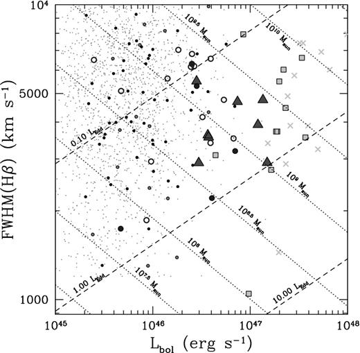
We show the Hβ emission-line FWHM versus the bolometric luminosity for several samples of quasars (tiny grey points: RL Shen et al. (2011); larger black dots: Shen et al. (2011) BALs; green dots: RL Shen et al. (2011) BALs; blue filled circles: BQS BALs; blue open circles: RL BQS; yellow filled squares: YW BALs; yellow crosses: RL YW; filled red triangles: radio-selected BALs from this work). Diagonal lines indicates black hole mass and Eddington ratio isopleths based on the Vestergaard & Peterson (2006) scaling relation. The bolometric luminosity is computed from the Runnoe et al. (2012) bolometric correction to the 5100 Å luminosity. The properties of radio-selected BALs do not stand out from the BQS and YW samples, and they are not super-accretors.
We calculate the correction to the scaling relationship for cosmology and find that it is negligible. Our black hole mass estimates are listed in Table 6 (column 3). For Eddington luminosity estimates, we use the relation LEdd = 1.51 × 1038(M/M⊙) erg s−1 (Krolik 1999).
These bolometric luminosity estimates as well as resulting estimating of the Eddington ratio are listed in Table 6 (columns 4 and 5).
We compare our sample to the higher redshift sample from YW and the lower redshift Bright Quasar Survey sample (BQS; Boroson & Green 1992) and Sloan Digital Sky Survey (SDSS) quasars from Shen et al. (2011). In order to facilitate the comparison, we re-calculate properties of interest for these samples in a consistent way. To calculate monochromatic luminosity at 5100 Å for the YW sample, we use the measured 3000 Å luminosities and a spectral index of αν = −0.44 (as is typical for quasars in this reshift range; Vanden Berk et al. 2001). For the BQS sample, we use the measured 9480 Å luminosities and spectral indices from Neugebauer et al. (1987). Shen et al. (2011) provide a measure of λLλ(5100 Å) that we adopt, although their average correction for host galaxy contamination warrants some discussion. All of the objects that we include from Shen et al. (2011) have redshifts less than 0.89, where objects with redshifts less than 0.5 are at risk for significant host contamination. In fact, the source luminosity is the important parameter for determining the fractional contribution to emission from the host galaxy, with low-luminosity sources prone to significant contamination. Shen et al. (2011) show that for sources with log λLλ(5100 Å) < 44.5 the host contributes of the order of a few per cent or less of the emission. For our bolometric correction this corresponds to log(Lbol) ≲ 45.5. The average host correction employed by Shen et al. (2011) may not be particularly accurate for individual objects, so the low-luminosity SDSS points where the host contributed a significant fraction of the total emission may be much more uncertain. Finally, to calculate bolometric luminosity in all samples, we applied the bolometric correction in equation (3).
The fact that our objects are not special in any particular parameter space is illustrated in Fig. 2, where we plot the Hβ FWHM versus bolometric luminosity (updating YW Fig. 2). We have placed isopleths of black hole mass (using the relation of Vestergaard & Peterson 2006) and Eddington ratio in the figure. The bolometric luminosities of our objects lie (mostly) below those of the higher redshift YW sample and above the lower redshift BQS and Shen et al. (2011) samples, as is completely expected for simple flux-limited surveys. This figure also clearly shows that neither radio-selected BAL quasars nor radio-quiet BAL quasars are exclusively super-accretors with Lbol/LEdd ≳ 1. We discuss this further below (Section 4).
We also consider the equivalent width ratio between the [O iii] λ5007 emission-line and the optical Fe ii emission-line complex. We follow the same method as Boroson & Green (1992) to calculate equivalent widths, taking the integrated flux of the emission line divided by the continuum flux at 4861 Å (the middle of the Hβ emission line). For the Fe ii flux, we integrate over the wavelength range 4434–4684 Å. In Fig. 3, we plot the cumulative distributions of the ratio for our sample and two subsamples from BQS (RL objects and radio-quiet BALs). Note that the BQS RL objects are typically more RL and cover a larger range in log(R*) than our sample. It is clear that the distribution of ratios for our radio-selected BALs differ greatly from the RL objects in the BQS [with mean ratios of 〈EW([O iii])/EW(Fe ii)〉 ≈ 0.1 and 1, respectively, and with only a 0.1 per cent Kolmogorov–Smirnov (KS) probability of being drawn from the same distribution]. On the other hand, the ratio resembles more the radio-quiet BALs from the BQS (〈EW([O iii])/EW(Fe ii)〉 ≈ 0.03), with a KS probability of 74 per cent of being drawn from the same parent distribution. The equivalent width ratio of [O iii] to Fe ii is essentially an estimate of an objects location on EV1, so this result supports the conclusion that RL BALs are more ‘BAL-like’ than ‘RL-like’.
![We show the cumulative probability distribution of the EW([O iii])/EW(Fe ii) equivalent-width ratio for three samples: our sample of radio-selected BAL quasars (bold solid line); 17 low-redshift RL objects from the BQS (Boroson & Green 1992, dashed black line) and 4 low-redshift, radio-quiet BAL quasars from the BQS (dot–dashed grey line). Arrows indicate objects that have only limits on the ratio from non-detection of either [O iii] or Fe ii. The limits are quoted at 3σ confidence.](https://oup.silverchair-cdn.com/oup/backfile/Content_public/Journal/mnras/433/2/10.1093/mnras/stt852/2/m_stt852fig3.jpeg?Expires=1749544493&Signature=FwoLPa3QOiRpYfr4eR5o6duY0MMdh8E5WXaB0dXi-teLErGULSzo3IVxLW3Sjlc8EHRobl6FT~teDke5fnSjXPUfOHczP-ofdK28WsGgkwfo1FtBP5Yyb8u3TNI9Tr~Q8hI2U8zUWOUC0UPYnsFggf39YqZBv7lqecNkV-ox45EO0brRSYYGcPGwPwjlAU7LZUlDV2hWqJYP7rnQmJwksS7Xee9kOuEOJ3kCWKtS0dy9oD0uGwaazgfaKChYqXnEFPaXGowJw8~7OFiH1lH8NBswhUaXlye3Vtxp49fGiD89BfaoOGYpcdtH8alO66UOSE~g-71Oda488512w5kJrQ__&Key-Pair-Id=APKAIE5G5CRDK6RD3PGA)
We show the cumulative probability distribution of the EW([O iii])/EW(Fe ii) equivalent-width ratio for three samples: our sample of radio-selected BAL quasars (bold solid line); 17 low-redshift RL objects from the BQS (Boroson & Green 1992, dashed black line) and 4 low-redshift, radio-quiet BAL quasars from the BQS (dot–dashed grey line). Arrows indicate objects that have only limits on the ratio from non-detection of either [O iii] or Fe ii. The limits are quoted at 3σ confidence.
3.2 A composite optical spectrum
To compare visually the general optical properties of radio-selected BAL quasars to other samples, we compute a composite spectrum from our eight quasars. To do so, we take the following steps: (1) Mask out pixels in the observed wavelength ranges 1.51–1.59 μm and 2.03–2.16 μm since these ranges cover the gaps between the J, H and K bands. (2) Use a cubic spline interpolation to place all spectra on the same rest-frame wavelength scale. The scale covers the range 3500–9000 Å in 3 Å bins. (3) Normalize the 5900–6000 Å average flux to unity. (4) For each wavelength bin, median combine the normalized flux from all spectra that have not been masked out at that wavelength.
The result of the compositing procedure is shown in Fig. 4. Two other composite spectra are also shown: RL quasars from the FBQS (Brotherton et al. 2001), and a composite of BAL quasars from Boroson & Green (1992) that have observed outflow velocities larger than 10 000 km s−1 (as listed in Laor & Brandt 2002). For this latter composite, we included the following quasars: PG 1700+518 (vmax = 31 000 km s−1), PG 2112+059 (vmax = 24 000 km s−1), PG 0043+039 (vmax = 19 000 km s−1), PG 1004+130 (vmax = 12 000 km s−1) and PG 1001+054 (vmax = 10 000 km s−1). To compute this composite, we use the same procedure as above except for step three, where we used the 4500–4510 Å flux to normalize the spectra. In addition, we have made measurements of the optical properties of the all three composites using basically the same specfit procedure as described above and listed them in Tables 4 and 5 (the results of the fit are also shown in Fig. 4).
![We show a composite optical spectrum of the eight IRTF/SpeX spectra of radio-selected BAL quasars (grey, solid histogram). In the top panel of the figure, we overlay the results of our spectral fit [total fit (red), Balmer emission (yellow), Fe ii template emission (green), [O iii] emission (blue), power-law continuum (orange)]. In the bottom panel, we show for comparison the composite quasar spectra of RL quasars (blue) from the FBQS (Brotherton et al. 2001), as well as a composite of low-redshift, radio-quiet BAL quasars from the BQS (red Boroson & Green 1992). All composites have been scaled to unit flux over the 5600–5680 Å wavelength range.](https://oup.silverchair-cdn.com/oup/backfile/Content_public/Journal/mnras/433/2/10.1093/mnras/stt852/2/m_stt852fig4.jpeg?Expires=1749544493&Signature=SLhwLQnbLNdYdu97UJhfcSxnQB06l1~leL-k9rpcdFqOXQReiIfrHbjEIUXdzaeo5~KvUTgouz3ozr2iVEgikreXJMfP5EPj8GcQKoQ5iK4Yfp-mV0kDCtSxGoO1gnpyDbV1XWIZEbWqnEz6l4paU7JB9y5qQBww~gRjpresHAfkNtsLbq519O7kdG4yiK277rynND3S8Ngf~PKU-EYGoEEuOfixZsJISf26MGqw6Qy7VvRLV4Xicgq-x0u~bxJ5Sw18~Y4EhumXPcWHSzskcSPPRpGjgUPsfXvBf4lxoV80MUZ1uumpxP79zZMfdd7UVNAziSnes6fiaE4sliRlyg__&Key-Pair-Id=APKAIE5G5CRDK6RD3PGA)
We show a composite optical spectrum of the eight IRTF/SpeX spectra of radio-selected BAL quasars (grey, solid histogram). In the top panel of the figure, we overlay the results of our spectral fit [total fit (red), Balmer emission (yellow), Fe ii template emission (green), [O iii] emission (blue), power-law continuum (orange)]. In the bottom panel, we show for comparison the composite quasar spectra of RL quasars (blue) from the FBQS (Brotherton et al. 2001), as well as a composite of low-redshift, radio-quiet BAL quasars from the BQS (red Boroson & Green 1992). All composites have been scaled to unit flux over the 5600–5680 Å wavelength range.
There were some differences in how the FBQS composite was fitted that resulted from the strong [O iii] and weak Fe ii. In addition to the two generally broad Gaussians, the fits to the Hβ and Hα emission lines included a narrow Gaussian to account for emission from the narrow-line region. This contribution is not included in the presented fit measurements. Additionally, the very strong λ5007 line required two Gaussians to achieve a good fit. These are combined in the presented fit measurements. In general, for both the FBQS and PG composites, the Fe ii template was not an excellent fit so the errors may be underestimated as a result.
4 RESULTS AND DISCUSSION
4.1 Results
From our analysis of rest-frame optical spectra of radio-selected BAL quasars, our main results are as follows.
[O iii] emission is weak, while optical Fe ii emission is strong. The optical spectra of radio-selected BAL quasars are more similar to radio-quiet BAL quasars than RL quasars (〈EW([O iii])/EW(Fe ii)〉 ≈ 0.1 and 0.03, respectively).
The physical properties of these quasars lie in the ranges: 0.1–0.9LEdd, (0.4–2.6) × 109 M⊙. We find that radio-selected BALs are not predominantly super-accretors.
There are two important comparisons to make in order to understand radio-selected BAL quasars and their role in the greater scheme of things. How do radio-selected BAL quasars compare to other BAL quasars? How do radio-selected BAL quasars compare to other RL objects? Of particular interest is the finding from previous studies (e.g. Becker et al. 2000) that radio-selected BAL quasars appear to show a range of orientations. What does this mean in terms of accretion physics? That is, do our objects add any insight into the interpretation of the Boroson & Green (1992) EV1? In the following subsections, we discuss these two points in light of our results.
4.2 The nature of radio-selected BALS compared to other quasars
The natural issue to consider given this sample is: How should this sample of radio-selected BAL quasars be treated in relation to other BAL quasars and RL objects? Because orientation can only be estimated in RL BAL quasars at this time, the answer to this question has implications for the extension of such considerations to radio-quiet BAL quasars.
Our results clearly show that the rest-frame optical properties of radio-selected BAL quasars are, essentially, indistinguishable from radio-quiet BAL quasars. Visually, this is most striking from the comparison of composite spectra in Fig. 4. [O iii] λ5007 emission is undetected, while optical Fe ii emission is very strong. This result is illustrated by Fig. 3 as well. By corollary, the optical properties of radio-selected BAL quasars do not mimic those of RL objects which tend to have strong [O iii] λ5007 and weak Fe ii emission. As noted earlier, DiPompeo et al. (2012a) also showed that the trends observed when comparing rest-frame spectral properties of BAL and non-BAL quasars persist whether the BALs are RL or radio quiet. Though not conclusive, as a direct RL/radio quiet comparison is lacking, this does suggest that the findings here extend to other wavelengths.
The radio luminosity, spectral index, and observed radio loudness of our targets are summarized in Table 1. Under the canonical loud/quiet divisions (e.g. Kellermann et al. 1994, RL: log R* > 1), all but two would be considered RL, though none fall into the class of truly radio-powerful (log R* > 2) and large FR II sources, though such sources do exist (e.g. Gregg et al. 2000; Brotherton et al. 2002; Gregg, Becker & de Vries 2006; Miller et al. 2009). Though radio selected, these BAL quasars tend to be considered radio intermediate, rather than truly RL. Nevertheless, the presence of radio emission is useful in gauging orientation. As already pointed out by Becker et al. (2000), the radio properties of these BAL quasars are consistent with a range of jet orientations. This finding has been confirmed for various other samples (Montenegro-Montes et al. 2008; Fine et al. 2011), as well as that of DiPompeo et al. (2011b) and DiPompeo, Brotherton & De Breuck (2012b) who find a slight dependence on orientation (at the largest viewing angles one is more likely to see a BAL). Moreover the RL BAL sources presented in this work have a very high fraction of compact radio sources unresolved in FIRST (about 90 per cent) compared with the parent population they were found within (about 60 per cent), a fact difficult to reconcile without invoking parameters in addition to viewing angle (such as age).
Should the results regarding the orientations of radio-selected BAL quasars be applied to all BAL quasars, the majority of which are truly radio quiet? Our results from looking at optical properties suggest that the answer is yes, as the RL BAL quasars are more ‘BAL-like’ than ‘RL-like’. While there have been suggestions in the past (e.g. Murray et al. 1995; Ogle et al. 1999; Elvis 2000) that BALs are seen in quasars at ‘large’, more edge-on inclination angles, the evidence supporting this perspective is circumstantial, and contradictory to the radio properties of radio-selected BAL quasars (Shankar et al. 2008; DiPompeo et al. 2011a, 2012a).
Of note, however, is that our sample of radio-selected BALs, like its parent sample from Becker et al. (2000), has a higher fraction of LoBALs and FeLoBALs than high-ionization BAL (HiBAL) quasars (see Table 2). There are no indications from the optical as to why these fractions would be different, either from the viewpoint of emission-line strengths, emission-line ratios or continuum shape. While optical polarization is generally higher in FeLoBALs/LoBALs (e.g. DiPompeo et al. 2010, 2013b), there appears to be no correlation with polarization and radio properties that would indicate FeLoBALs/LoBALs are seen from the largest viewing angles. Our findings here indicate that study of the full BAL subclass, from radio quiet to RL, should move away from the simplest orientation-based explanations.
Whether or not differences in geometry or age exist, differences in the radio properties of the BAL quasar population compared to other quasars clearly do exist given that at the largest viewing angles BALs are more likely to be observed (DiPompeo et al. 2012b) and that the presence of BALs depends on radio power (Shankar et al. 2008; Dai, Shankar & Sivakoff 2012). Moreover, the optical properties do not span the full range seen in non-BAL quasars, no matter the radio loudness, which we discuss in the next section.
4.3 EV1 versus accretion rate: BALQSOs and low [O iii]/Fe ii
A picture is emerging in which BAL quasars, including radio-selected BAL quasars, display spectral properties at the well-defined, extreme end of EV1, with weak [O iii] and strong Fe ii (e.g. Boroson & Green 1992). In a sample selected to have weak [O iii], Turnshek et al. (1997) found that a third of their objects had BALs, twice the normal 15 per cent (Gibson et al. 2009). At the opposite extreme of EV1 spectral properties, BALs are simply not observed.
From Fig. 2, the radio-selected BAL quasars in this sample have bolometric luminosities in between those of the YW sample and the low-redshift (z < 0.5) objects from the Palomar–Green catalogue (Boroson & Green 1992) and z < 0.89 SDSS quasars from Shen et al. (2011). Moreover, the estimates of Eddington ratio are not indicative of extreme accretion; only one object, Q1031+3953, has an Eddington ratio larger than unity. This is curious since EV1 for low-redshift objects appears to be correlated strongly with Eddington ratio in the sense that objects with strong Fe ii emission and weak [O iii] emission should be accreting near the Eddington luminosity (Boroson 2002). Written before many RL BALs had been discovered, that work suggested that RL BALs should show extremely high Eddington ratios. It is possible that EV1 behaves differently at different redshifts. This would explain why the sample of Boroson (2002), with redshifts of a few tenths or less, shows a strong correlation between EV1 and Eddington ratio that is not confirmed in higher redshift samples, namely ours (z ∼ 0.7–2.4) and the YW sample (z ∼ 2).
A clue to this mystery may be found in considering the dominant parameters that define EV1. In terms of [O iii] and Fe ii strength, our sample resembles radio-quiet BALs which would have small/low values of EV1. The Boroson (2002) EV1 also involves other parameters, including the Hβ emission-line FWHM and formal radio loudness. Our objects only represent an extreme of [O iii] and the Fe ii strengths, the dominant EV1 parameters, and not these other properties.
Multiple physical drivers for EV1 have been put forth in the literature. At low redshift, using the Palomar–Green sample with z < 0.5, Boroson & Green (1992) find that Eddington ratio dominates the variation of optical properties, and hence EV1, but at higher redshift this is not the case. Since there is a common feature that [O iii] emission is weak and Fe ii emission is strong in BAL quasars of any redshift, YW suggest that the availability of cold gas may be important in considering the relationship between BAL quasars and EV1. The anticorrelation between [O iii] and Fe ii emission may be a more fundamental relationship among quasars (i.e. at any redshift/luminosity). However, the entirety of EV1 as defined by low-z objects and its correlation with Eddington ratio might be secondary. Further drivers include the suggestion that EV1 should be correlated with the ratio of optical to mid-infrared emission, which is indicative of the amount of reprocessed optical emission that should scale with the covering fraction of dust. DiPompeo et al. (2013b) finds an infrared excess in RL BAL quasars consistent with such a prediction. Wills et al. (1999) found that some of the line ratios associated with EV1 were diagnostic of gas density, and that property may be involved as well. Our analysis, where we find that RL BAL quasars exhibit spectral properties on the extreme end of EV1 but not necessarily extremely high Eddington ratios, rules out the Eddington fraction as a driver of EV1, at least at high redshift. With such varied evidence, it is clear that the physical driver of EV1 remains elusive.
5 CONCLUSIONS
We have observed the rest-frame optical properties of eight radio-selected BAL quasars from Becker et al. (2000) using the NASA IRTF/SpeX instrument. Using the specfit package, we have separated the power-law continuum, Fe ii emission, [O iii] emission, Hα and Hβ emission. Furthermore, we have estimated the black hole masses and Eddington ratios of these quasars. Radio-selected BAL quasars have similar optical properties (weak [O iii], strong Fe ii) as radio-quiet BAL quasars and are dissimilar to RL non-BAL quasars in this sense. In short, RL BAL quasars are more ‘BAL-like’ than ‘RL-like’. As these objects are not extreme accretors, we conclude that the properties defining EV1 at low redshift may not be directly extrapolated to high redshift/luminosity objects. The anticorrelation between [O iii] and Fe ii emission may be fundamental with BAL quasars lying at one extreme, but this is not necessarily a result of Eddington ratio.
We wish to thank Bev Wills for helpful discussions and assistance with reduction of the IRTF data and the anonymous referee for helpful and detailed comments that improved the presentation of this work. This work was part of the Wyoming SURAP REU programme funded by the National Science Foundation grant ASTR-0353760. We acknowledge support from the US National Science Foundation through grant AST 05-07781. ZS acknowledges the support from the National Natural Science Foundation of China through grant 10633040.
This publication makes use of data products from the Two Micron All Sky Survey, which is a joint project of the University of Massachusetts and the Infrared Processing and Analysis Center/California Institute of Technology, funded by the National Aeronautics and Space Administration and the National Science Foundation.
Funding for the SDSS and SDSS-II has been provided by the Alfred P. Sloan Foundation, the Participating Institutions, the National Science Foundation, the US Department of Energy, the National Aeronautics and Space Administration, the Japanese Monbukagakusho, the Max Planck Society and the Higher Education Funding Council for England. The SDSS website is http://www.sdss.org/.
The SDSS is managed by the Astrophysical Research Consortium for the Participating Institutions. The Participating Institutions are the American Museum of Natural History, Astrophysical Institute Potsdam, University of Basel, University of Cambridge, Case Western Reserve University, University of Chicago, Drexel University, Fermilab, the Institute for Advanced Study, the Japan Participation Group, Johns Hopkins University, the Joint Institute for Nuclear Astrophysics, the Kavli Institute for Particle Astrophysics and Cosmology, the Korean Scientist Group, the Chinese Academy of Sciences (LAMOST), Los Alamos National Laboratory, the Max-Planck-Institute for Astronomy (MPIA), the Max-Planck-Institute for Astrophysics (MPA), New Mexico State University, Ohio State University, University of Pittsburgh, University of Portsmouth, Princeton University, the United States Naval Observatory and the University of Washington.
iraf is distributed by the National Optical Astronomy Observatories, which are operated by the Association of Universities for Research in Astronomy, Inc., under cooperative agreement with the National Science Foundation.
