


Abstract
The current helicity in solar active regions derived from vector magnetograph observations for more than 20 years indicates the so-called hemispheric sign rule; the helicity is predominantly negative in the Northern hemisphere and positive in the Southern hemisphere. In this paper, we revisit this property and compare the statistical distribution of current helicity with Gaussian distribution using the method of normal probability paper. The data sample comprises 6630 independent magnetograms obtained at Huairou Solar Observing Station, China, over 1988–2005 which correspond to 983 solar active regions. We found the following. (1) For the most of cases in time-hemisphere domains the distribution of helicity is close to Gaussian. (2) At some domains (some years and hemispheres) we can clearly observe significant departure of the distribution from a single Gaussian, in the form of two- or multicomponent distribution. (3) For the most non-single-Gaussian parts of the data set we see coexistence of two or more components, one of which (often predominant) has a mean value very close to zero, which does not contribute much to the hemispheric sign rule. The other component has relatively large value of helicity that often determines agreement or disagreement with the hemispheric sign rule in accord with the global structure of helicity reported by Zhang et al.
1 INTRODUCTION
Recently there has been significant progress in collection and interpretation of observational data on vector magnetic fields in solar active regions which enables us to compute the values of current helicity (a measure of departure of magnetic fields from mirror symmetry) averaged over active regions (Seehafer 1990; Pevtsov, Canfield & Metcalf 1995; Bao & Zhang 1998). The data have been averaged over latitude and time in the solar cycle as well (Zhang et al. 2010). The research so far has demonstrated important properties of this quantity and its regular variation in the course of the solar cycle. The helicity is generally negative in the Northern hemisphere and positive in the Southern hemisphere; the so-called hemispheric sign rule (HSR) for helicity. This rule, however, may occasionally be violated in the activity minimum periods (Hagino & Sakurai 2005; Zhang et al. 2010; Hao & Zhang 2012).
Helicity in the solar atmosphere has been noted as an important agent which constrains magnetic field dissipation in the solar corona. Current helicity plays an important role in the solar dynamo theory as an observational proxy of the α-effect as it controls a dynamical back-reaction of the magnetic field to the motion of the media which suppresses and stabilizes the generation of the magnetic field (e.g. Kleeorin et al. 2003; Zhang et al. 2006). From a theoretical point of view the average helicity has the meaning of a quantity averaged over an ensemble of turbulent fluctuations in a small physical volume. This physical volume may contain a limited number of convective cells, and so we may expect it to vary significantly in space and time. The data on current helicity are indeed very fluctuating within a given active region as well as during its evolution (Zhang, Bao & Kuzanyan 2002). Similar fluctuations can be observed in the current helicity averaged over latitude and time in the solar cycle.
However, the observation of current helicity is a complex process which deals with initially imperfect data and involves highly non-trivial reduction processes. These difficulties must be overcome by collecting reliable data sets, because noise in the data will degrade the reliability in the analysis (e.g. Abramenko, Wang & Yurchishin 1996; Bao & Zhang 1998; Bao, Ai & Zhang 2001; Hagino & Sakurai 2004, 2005). For better understanding of the reliability of the analysis of current helicity previously undertaken, we hereby aim to study its statistical distribution.
On the other hand the current helicity as a quantity responsible for mirror asymmetry of solar magnetic field is expected to be fluctuating also from a theoretical viewpoint. A usual expectation is that the degree of mirror asymmetry in dynamo mechanisms will be about 10 per cent. This practical estimate as originating from Parker (1955) means that we have to isolate stable features of current helicity distributions on a background of physical fluctuation which may be 10 times greater than the average value. This fluctuation is not due to observational uncertainties and cannot be reduced by improvement of observational techniques.
The expected substantial fluctuation in the current helicity data has to be carefully taken into account in estimating the averaged values of current helicity. Intrinsic (physical and true) dispersion in the current helicity data around its mean value is, however, interesting by itself.
The probability distribution of current helicity may be substantially non-Gaussian. The point is that physical processes responsible for the fluctuating nature of solar plasma can be considered as an action of a product of independent evolutionary operators rather than a sum of them resulting usually in a Gaussian distribution. On the other hand, averaging over an active region smoothes fluctuation and supports the Gaussian nature of distribution.
Because of this, the statistical properties of current helicity deserve to be addressed in full detail. Previously, the statistical distribution of current helicity has been addressed only briefly as a part of more general studies (e.g. Sokoloff et al. 2008).
In this paper, we consider the distribution of available data over the hemispheres of the Sun and their changes over solar cycles. We compare this distribution with a Gaussian and separate the part of the data which significantly deviates from a single Gaussian distribution. Then, we consider the spatial and temporal properties of this part in comparison with the other (Gaussian) part of the data. We shall see that both parts exhibit similar properties and behaviour over the solar cycle.
2 OBSERVATIONAL DATA SET
This study is based on the data of photospheric vector magnetograms of solar active regions obtained at Huairou Solar Observing Station, China. The same data base systematically covering 18 consecutive years (1988–2005) was used in Zhang et al. (2010). The parameters adopted there are αav (the average value of α; |$\nabla \times {\boldsymbol B} =\alpha {\boldsymbol B}$|) and Hc (the integrated current helicity; Hc = ΣJzBz). In the present analysis we will use the same parameters (the integrated current helicity; Hc = σJzBz). First, we analyse the entire data base that comprises 6630 magnetograms of 983 different active regions (in terms of NOAA region numbers). We are going to build our statistical analysis for the whole bulk of available data. The majority of active regions are represented by only one or very few magnetograms. However, there are a few active regions that were recorded in 20 or more magnetograms. In the next step we select one magnetogram for an active region. Sometimes, and for some active regions that were observed within a short time interval, the helicity parameters may be close with each other. For these magnetograms, we select the one located nearest to the centre of the solar disc. Furthermore, we try to avoid choosing the magnetograms of rapidly emerging active regions, except for those regions which were recorded in only one magnetogram. Nonetheless, this occurs rather rarely because such active regions are usually large and well observed over several days.
3 METHOD OF STATISTICAL ANALYSIS
We address the probability distribution of current helicity and its deviation from Gaussian as it follows from observational data by two statistical tools.
First of all, we divide the data into two hemispheres and produce histograms of the current helicity distribution for certain time intervals which contain 50 measurements. We then approximate them by multiple Gaussians. In practice it appears that a mixture of two Gaussians is sufficient to reproduce the histograms with a reasonable accuracy.
This method, being very practical, may miss in principle substantial deviations from Gaussian statistics which occurs with low probability, i.e. intermittent features in the probability distribution. A tool to address an intermittent feature is the so-called Normal Probability Paper (NPP) test which is organized as follows (see e.g. Chernoff & Lieberman 1954).
Let our set contain N active regions. Let n active regions have current helicity density χc lower than x. Then the probability for χc to be lower than x is estimated as P = n/N. Let ξ be a Gaussian variable with the same mean value μ and standard deviation σ as χc and let y be the value for which the probability for (ξ − μ)/σ to be lower than y is P. The results for various x values are plotted in the (x, y) plane and can be compared with the cumulative distribution function (CDF) for a Gaussian distribution which gives a straight line in this coordinate space. If the observational data deviate substantially from this straight line, it is an indication of a non-Gaussian nature of observational data (see e.g. Sokoloff et al. 2008 for details).
For illustration let us produce a set of random Gaussian variable xx1 (N = 1500, μ1 = 0.098 and σ1 = 1.05) by idl function ‘random’. Then we produce another set of random Gaussian variable xx2 (μ2 = −0.28 and σ2 = 0.42). The GAUSS_CVF function computes the cutoff value V in a standard Gaussian distribution with a mean of 0.0 and a variance of 1.0 such that the probability that a random variable X is greater than V is equal to a user-supplied probability P (see Fig. 1). The upper panel shows the probability distribution functions (PDFs) of two Gaussian components and their sum (with equal weights). In the bottom panel, we show the relationship between the variable and the Gaussian CDF with the same mean value and standard deviation for three kinds of variables. The correlation for Gaussian variables is well fit by a straight line but not for the sum of the components, as shown in Fig. 1 by the red curve. The slope of the straight line is determined by the mean value, and the y-intercept is determined by the standard deviation of the corresponding data set.
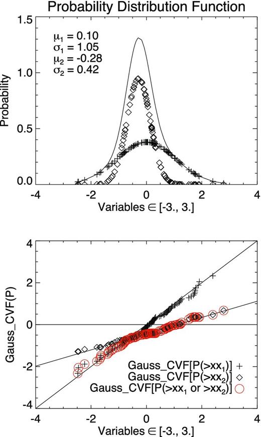
Probability distribution function of a set of random Gaussian variable (upper panel) and correlation between the variable and the Gaussian cumulative distribution function with the same mean value and standard deviation (bottom panel).
4 RESULTS
Results of fitting to the data of αav for 10 data sub-groups in the Northern hemisphere. The fit error is standard deviation of the fitting curve from the observed values. The values of amplitudes A1 and A2 for cases when the second components is significant (A2 > A1/2) are underlined.
| |$\#$| | Start | End | δT | μ0 | σ0 | μ1 | σ1 | A1 | μ2 | σ2 | A2 | Error | No |
|---|---|---|---|---|---|---|---|---|---|---|---|---|---|
| 1 | 1988-Apr-16 | 1990-May-11 | 755 | −0.0088 | 0.0176 | −0.0046 | 0.0154 | 0.8932 | −0.0405 | 0.0061 | 0.1068 | 0.0948 | 50 |
| 2 | 1990-May-20 | 1992-Jan-22 | 612 | −0.0119 | 0.0231 | −0.0057 | 0.0160 | 0.6506 | −0.0226 | 0.0347 | 0.3494 | 0.1356 | 50 |
| 3 | 1992-Jan-25 | 1993-Dec-18 | 693 | 0.0021 | 0.0227 | −0.0031 | 0.0071 | 0.5360 | 0.0094 | 0.0353 | 0.4640 | 0.1364 | 50 |
| 4 | 1993-Dec-26 | 1998-May-24 | 1610 | −0.0065 | 0.0169 | −0.0044 | 0.0231 | 0.5651 | −0.0082 | 0.0088 | 0.4349 | 0.1840 | 50 |
| 5 | 1998-May-31 | 1999-Jul-22 | 417 | −0.0042 | 0.0161 | −0.0034 | 0.0126 | 0.9609 | −0.0843 | 0.0055 | 0.0391 | 0.1330 | 50 |
| 6 | 1999-Jul-23 | 2000-Jun-11 | 324 | −0.0030 | 0.0128 | −0.0026 | 0.0176 | 0.5978 | −0.0029 | 0.0058 | 0.4022 | 0.1127 | 50 |
| 7 | 2000-Jun-12 | 2000-Dec-21 | 192 | −0.0046 | 0.0140 | −0.0016 | 0.0091 | 0.8807 | −0.0402 | 0.0287 | 0.1193 | 0.1369 | 50 |
| 8 | 2000-Dec-25 | 2001-Sep-02 | 251 | 0.0005 | 0.0200 | 0.0035 | 0.0306 | 0.5017 | −0.0015 | 0.0071 | 0.4983 | 0.1204 | 50 |
| 9 | 2001-Sep-22 | 2003-Jun-28 | 644 | −0.0038 | 0.0177 | −0.0045 | 0.0168 | 0.9779 | 0.2665 | 0.3073 | 0.0221 | 0.1293 | 50 |
| 10 | 2003-Jul-5 | 2005-Dec-23 | 902 | −0.0028 | 0.0123 | −0.0057 | 0.0211 | 0.5652 | 0.0008 | 0.0035 | 0.4348 | 0.2200 | 14 |
Table 1 shows the result of Gaussian fitting/decomposition for αav in the Northern hemisphere. We focus on the relation between the sign of mean values of two Gaussian components and the HSR. It is found that there are merely one μ1 (Row 8) which violates the HSR from 2000-Dec-25 to 2001-Sep-02, while the corresponding μ2 follows the HSR. In contrast, there are in total three μ2's (Rows 3, 9 and 10) which violate the HSR. These epochs are ‘1992-Jan-25’ to ‘1993-Dec-18’, ‘2001-Sep-22’ to ‘2003-Jun-28’ and ‘2003-Jul-5’ to ‘2005-Dec-23’, and their amplitudes A2 are 0.46, 0.02 and 0.43, respectively. We would like to stress here that the number of data points in the latter sub-group is only 14, which is much less than in the other sub-groups. Therefore, the fitting for this sub-group is not that reliable. Nevertheless, the fitting in the third sub-group, i.e. from ‘1992-Jan-25’ to ‘1993-Dec-18’, is rather convincing. As A2 is 0.46 for the former group, both components are clearly seen in the second row of Fig. 2. In Fig. 2, we also give fitting results for the other three epochs. Their distributions are nicely represented by two Gaussians and both components obey the HSR.

Four cases of the distributions of αav in the Northern hemisphere. The left-hand panels show NPP and are annotated by the start and ending dates of the group. The right-hand panels show the data histogram and decomposed two Gaussians (dotted curves) and their sum (solid curve).
Table 2 shows the results of Gaussian fitting/decomposition for αav in the Southern hemisphere. It is found that four μ1's and three μ2's violate the HSR. Among them, two cases have both μ1 and μ2 violate the HSR. They occur in the epochs ‘1988-Apr-26’ to ‘1990-Feb-25’ and ‘1999-May-19’ to ‘2000-Apr-12’, respectively. The amplitudes of A1 are 0.82 and 0.96 and A2 are 0.18 and 0.04, respectively. Other two A2 that violate HSR have amplitudes of 0.04 and 0.02, respectively. Some examples are given in Fig. 3. The first row shows apparent violation of two components from the HSR. Other three cases show two components clearly, too. However, all of these components obey the HSR.
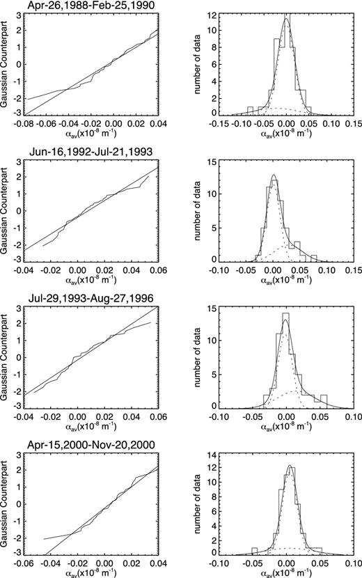
Four cases of the distributions of αav in the Southern hemisphere. The left-hand panels show NPP and are annotated by the start and ending dates of the group. The right-hand panels show the data histogram and decomposed two Gaussians (dotted curves) and their sum (solid curve).
Results of fitting to the data of αav for 11 data sub-groups in the Southern hemisphere. The fit error is standard deviation of the fitting curve from the observed values. The values of amplitudes A1 and A2 for cases when the second component is significant (A2 > A1/2) are underlined.
| |$\#$| | Start | End | δT | μ0 | σ0 | μ1 | σ1 | A1 | μ2 | σ2 | A2 | Error | No |
|---|---|---|---|---|---|---|---|---|---|---|---|---|---|
| 1 | 1988-Apr-26 | 1990-Feb-25 | 670 | −0.0039 | 0.0235 | −0.0003 | 0.0181 | 0.8223 | −0.0227 | 0.0487 | 0.1777 | 0.0993 | 50 |
| 2 | 1990-Mar-08 | 1991-Aug-11 | 521 | 0.0068 | 0.0254 | 0.0027 | 0.0162 | 0.8035 | 0.0283 | 0.0542 | 0.1965 | 0.1364 | 50 |
| 3 | 1991-Aug-12 | 1992-May-08 | 270 | 0.0053 | 0.0165 | 0.0020 | 0.0198 | 0.6668 | 0.0128 | 0.0096 | 0.3332 | 0.0807 | 50 |
| 4 | 1992-Jun-16 | 1993-Jul-21 | 400 | 0.0090 | 0.0206 | 0.0008 | 0.0123 | 0.6766 | 0.0287 | 0.0266 | 0.3234 | 0.0931 | 50 |
| 5 | 1993-Jul-29 | 1996-Aug-27 | 1125 | 0.0038 | 0.0188 | −0.0019 | 0.0106 | 0.6147 | 0.0147 | 0.0279 | 0.3853 | 0.0895 | 50 |
| 6 | 1996-Nov-29 | 1999-Apr-23 | 875 | 0.0053 | 0.0155 | 0.0053 | 0.0208 | 0.6437 | 0.0063 | 0.0057 | 0.3563 | 0.1044 | 50 |
| 7 | 1999-May-19 | 2000-Apr-12 | 329 | −0.0010 | 0.0118 | −0.0001 | 0.0091 | 0.9575 | −0.0587 | 0.0056 | 0.0425 | 0.1029 | 50 |
| 8 | 2000-Apr-15 | 2000-Nov-20 | 219 | 0.0048 | 0.0160 | 0.0050 | 0.0110 | 0.7850 | 0.0044 | 0.0351 | 0.2150 | 0.0927 | 50 |
| 9 | 2000-Nov-27 | 2001-Oct-11 | 318 | 0.0022 | 0.0231 | 0.0011 | 0.0122 | 0.6237 | 0.0053 | 0.0399 | 0.3763 | 0.1328 | 50 |
| 10 | 2001-Oct-22 | 2003-Oct-27 | 735 | 0.0002 | 0.0170 | 0.0017 | 0.0163 | 0.9807 | −0.0694 | 0.0039 | 0.0193 | 0.0992 | 50 |
| 11 | 2003-Oct-28 | 2005-Dec-16 | 780 | −0.0045 | 0.0166 | −0.0070 | 0.0238 | 0.6532 | 0.0010 | 0.0074 | 0.3468 | 0.1287 | 19 |
We also perform comparative analysis for Hc in a similar way. Table 3 shows the fitting results in the Northern hemisphere. For example, in Row 3, i.e. from 1992-Jan-25 to 1993-Dec-18, the means of both components μ1 and μ2 show violation of the HSR. Their amplitudes are 0.91 and 0.09. This is also consistent with the results obtained for αav. Some examples are given in Fig. 4.
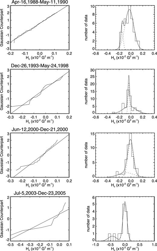
Four cases of the distributions of Hc in the Northern hemisphere. The left-hand panels show NPP and are annotated by the start and ending dates of the group. The right-hand panels show the data histogram and decomposed two Gaussians (dotted curves) and their sum (solid curves).
Results of fitting to the data of Hc for 10 sub-groups in the Northern hemisphere.
| |$\#$| | Start | End | δT | μ0 | σ0 | μ1 | σ1 | A1 | μ2 | σ2 | A2 | Error | No |
|---|---|---|---|---|---|---|---|---|---|---|---|---|---|
| 1 | 1988-Apr-16 | 1990-May-11 | 755 | −0.0421 | 0.0758 | −0.0268 | 0.0741 | 0.8927 | −0.1492 | 0.0198 | 0.1073 | 0.0860 | 50 |
| 2 | 1990-May-20 | 1992-Jan-22 | 612 | −0.0774 | 0.2541 | −0.0347 | 0.0953 | 0.8894 | −0.8641 | 0.5144 | 0.1106 | 0.0688 | 50 |
| 3 | 1992-Jan-25 | 1993-Dec-18 | 693 | 0.0544 | 0.2714 | 0.0157 | 0.1149 | 0.9140 | 0.5670 | 0.9986 | 0.0860 | 0.1649 | 50 |
| 4 | 1993-Dec-26 | 1988-May-24 | 1610 | −0.0319 | 0.0814 | −0.0268 | 0.1084 | 0.6583 | −0.0355 | 0.0132 | 0.3417 | 0.2020 | 50 |
| 5 | 1998-May-31 | 1999-Jul-22 | 417 | −0.0187 | 0.0860 | −0.0094 | 0.0668 | 0.9321 | −0.3537 | 0.1570 | 0.0679 | 0.0822 | 50 |
| 6 | 1999-Jul-23 | 2000-Jun-11 | 324 | −0.0078 | 0.0651 | −0.0050 | 0.0748 | 0.8629 | −0.0139 | 0.0223 | 0.1371 | 0.1012 | 50 |
| 7 | 2000-Jun-12 | 2000-Dec-21 | 192 | −0.0267 | 0.0753 | −0.0064 | 0.0476 | 0.7282 | −0.0816 | 0.1299 | 0.2718 | 0.1168 | 50 |
| 8 | 2000-Dec-25 | 2001-Sep-02 | 251 | −0.0154 | 0.0677 | −0.0043 | 0.0480 | 0.9682 | −0.3474 | 0.0013 | 0.0318 | 0.1337 | 50 |
| 9 | 2001-Sep-22 | 2003-Jun-28 | 644 | −0.0228 | 0.1047 | −0.0075 | 0.1297 | 0.7312 | −0.0536 | 0.0287 | 0.2688 | 0.0991 | 50 |
| 10 | 2003-Jul-5 | 2005-Dec-23 | 902 | −0.0817 | 0.1614 | −0.0030 | 0.0675 | 0.7956 | −0.4294 | 0.1380 | 0.2044 | 0.0679 | 14 |
Table 4 shows the results of Gaussian fitting/decomposition for Hc in the Southern hemisphere. There are three μ1's that violate the HSR in Rows 1, 7 and 11, respectively. Their amplitudes are 0.94, 0.68 and 0.89, respectively. In Rows 1 and 11, the second components also violate the HSR, though with smaller component amplitudes of 0.06 and 0.11. Another μ2 violating the HSR occurs in the epoch of ‘1990-Mar-08’ to ‘1991-Aug-11’ (in Row 2); its amplitude is 0.11. Some examples are given in Fig. 5.
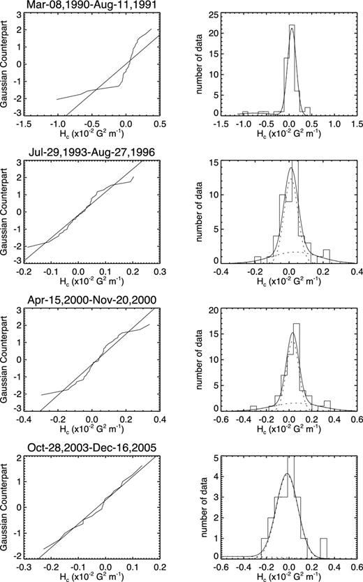
Four cases of the distributions of Hc in the Southern hemisphere. The left-hand panels show NPP and are annotated by the start and ending dates of the group. The right-hand panels show the data histogram and decomposed two Gaussians (dotted curves) and their sum (solid curve).
Results of fitting to the data of Hc for 11 data sub-groups in the Southern hemisphere.
| |$\#$| | Start | End | δT | μ0 | σ0 | μ1 | σ1 | A1 | μ2 | σ2 | A2 | Error | No |
|---|---|---|---|---|---|---|---|---|---|---|---|---|---|
| 1 | 1988-Apr-26 | 1990-Feb-25 | 670 | −0.0273 | 0.1756 | −0.0004 | 0.1008 | 0.9426 | −0.8515 | 0.1035 | 0.0574 | 0.1190 | 50 |
| 2 | 1990-Mar-08 | 1991-Aug-11 | 521 | 0.0061 | 0.2285 | 0.0622 | 0.0956 | 0.8886 | −0.7620 | 0.3935 | 0.1114 | 0.1403 | 50 |
| 3 | 1991-Aug-12 | 1992-May-08 | 270 | 0.0492 | 0.1122 | 0.0514 | 0.1234 | 0.9488 | 0.0628 | 0.0078 | 0.0512 | 0.0931 | 50 |
| 4 | 1992-Jun-16 | 1993-Jul-21 | 400 | 0.1195 | 0.2721 | 0.0810 | 0.1102 | 0.9185 | 0.6108 | 1.0473 | 0.0815 | 0.2526 | 50 |
| 5 | 1993-Jul-29 | 1996-Aug-27 | 1125 | 0.0176 | 0.0735 | 0.0115 | 0.0409 | 0.6867 | 0.0369 | 0.1377 | 0.3133 | 0.1160 | 50 |
| 6 | 1996-Nov-29 | 1999-Apr-23 | 875 | 0.0331 | 0.0810 | 0.0130 | 0.0644 | 0.8737 | 0.1903 | 0.0312 | 0.1263 | 0.0989 | 50 |
| 7 | 1999-May-19 | 2000-Apr-12 | 329 | 0.0053 | 0.0708 | −0.0045 | 0.0386 | 0.6750 | 0.0317 | 0.1284 | 0.3250 | 0.0963 | 50 |
| 8 | 2000-Apr-15 | 2000-Nov-20 | 219 | 0.0385 | 0.1084 | 0.0313 | 0.0547 | 0.6922 | 0.0617 | 0.2106 | 0.3078 | 0.1359 | 50 |
| 9 | 2000-Nov-27 | 2001-Oct-11 | 318 | 0.0254 | 0.0807 | 0.0141 | 0.0438 | 0.8746 | 0.1172 | 0.2507 | 0.1254 | 0.1711 | 50 |
| 10 | 2001-Oct-22 | 2003-Oct-27 | 735 | 0.0198 | 0.1427 | 0.0213 | 0.0527 | 0.5970 | 0.0260 | 0.2490 | 0.4030 | 0.1354 | 50 |
| 11 | 2003-Oct-28 | 2005-Dec-16 | 780 | −0.0133 | 0.1155 | −0.0173 | 0.0949 | 0.8855 | −0.4921 | 0.4071 | 0.1145 | 0.0873 | 19 |
To compare the epochs where the HSR is violated in the present statistical analysis with the evolution and distribution of αav and Hc obtained in our earlier papers (Zhang et al. 2010), we mark these epochs with the inclined lines of 45° (the first component violates the HSR) and −45° (the second component violates the HSR); see Fig. 6. Therefore, the crossed lines represent the cases when both the first and the second components violate the HSR.
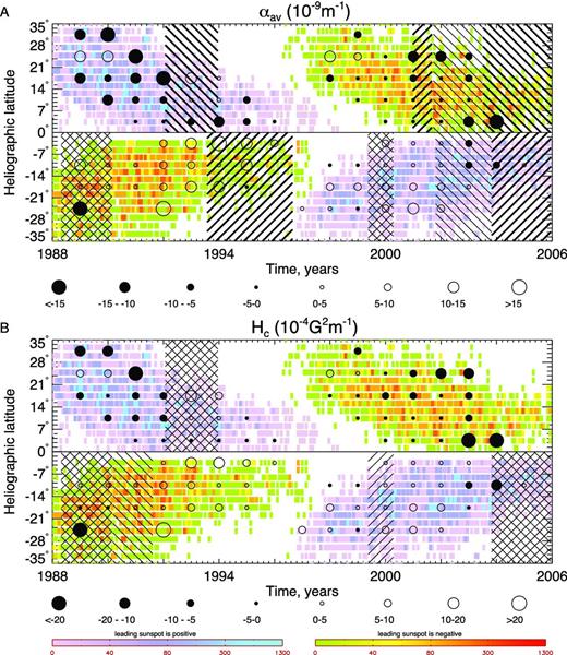
Time-latitude distribution of Gaussian components for selected 983 magnetograms of active regions (one magnetogram per active region) over the period of 1988–2005. The background is the butterfly diagram of current helicity plotted in time-latitude bins as circles over the colour plot of sunspot number density. Each bin contains data coming from 7° in latitude and two year running average in time. The 45° and −45° lines mark the epoch in which the main component and sub-component violate the HSR, respectively. The thick lines denote cases when the second component is significant, i.e. the amplitudes satisfy the relation A1 < 2A2. The upper and lower panels show the results for αav and Hc, respectively.
Here, we estimate the uncertainty in determination of the two Gaussian mean values of the bi-modal distribution of the two parameters αav and Hc under discussion. For that we use the 95 per cent Student's confidence intervals taking the standard deviations for each Gaussian component σi, where i = 1, 2, and computing the number of degrees of freedom as the overall number of available data points in each interval n minus the number of fitting parameters, namely five. Then the expected errors in the mean values of the components would be |$\mu _i \pm {\sigma _i t_{n-5}}/{\sqrt{n-5}}$|, where tn − 5 is Student's quantile for 95 per cent probability. We consider the violation of the rule significant if the error bars on the mean values that violate the HSR do not contain the zero value of the quantity under consideration. The results are shown in Tables 5– 8. The mean values which violate the HSR are shown bold, and the cases of significant violation are underlined. The cases for which violation of the HSR is statistically significant are shown in Fig. 7.
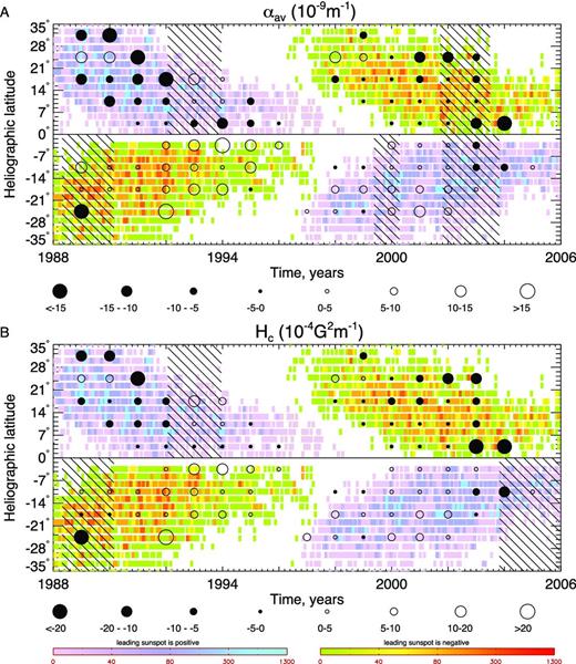
Butterfly diagram with only those cases marked for which violation of the HSR is statistically significant. Notations are the same as in Fig. 6.
Statistical significance of HSR violation for α in the Northern hemisphere. Numbers in bold indicate violation of HSR, and they are underlined if regarded statistically significant.
| |$\#$| | Start | End | μ1 | |$\frac{\sigma _1 t_{n-5}}{\sqrt{n-5}}$| | μ2 | |$\frac{\sigma _2 t_{n-5}}{\sqrt{n-5}}$| | |||
|---|---|---|---|---|---|---|---|---|---|
| 3 | 1992-Jan-25 | 1993-Dec-18 | −0.0031 | 0.0018 | 0.0094 | 0.0088 | |||
| 8 | 2000-Dec-25 | 2001-Sep-02 | 0.0035 | 0.0077 | −0.0015 | 0.0018 | |||
| 9 | 2001-Sep-22 | 2003-Jun-28 | −0.0045 | 0.0042 | 0.2665 | 0.0769 | |||
| 10 | 2003-Jul-5 | 2005-Dec-23 | −0.0057 | 0.0129 | 0.0008 | 0.0021 |
Statistical significance of HSR violation for α in the Southern hemisphere. Numbers in bold indicate violation of HSR, and they are underlined if regarded statistically significant.
| |$\#$| | Start | End | μ1 | |$\frac{\sigma _1 t_{n-5}}{\sqrt{n-5}}$| | μ2 | |$\frac{\sigma _2 t_{n-5}}{\sqrt{n-5}}$| | |||
|---|---|---|---|---|---|---|---|---|---|
| 1 | 1988-Apr-26 | 1990-Feb-25 | −0.0003 | 0.0045 | −0.0227 | 0.0122 | |||
| 5 | 1993-Jul-29 | 1996-Aug-27 | −0.0019 | 0.0026 | 0.0147 | 0.0070 | |||
| 7 | 1999-May-19 | 2000-Apr-12 | −0.0001 | 0.0023 | −0.0587 | 0.0014 | |||
| 10 | 2001-Oct-22 | 2003-Oct-27 | 0.0017 | 0.0041 | −0.0694 | 0.0010 | |||
| 11 | 2003-Oct-28 | 2005-Dec-16 | −0.0070 | 0.0136 | 0.0010 | 0.0042 |
Statistical significance of HSR violation for Hc in the Northern hemisphere. Numbers in bold indicate violation of HSR, and they are underlined if regarded statistically significant.
| |$\#$| | Start | End | μ1 | |$\frac{\sigma _1 t_{n-5}}{\sqrt{n-5}}$| | μ2 | |$\frac{\sigma _2 t_{n-5}}{\sqrt{n-5}}$| | |||
|---|---|---|---|---|---|---|---|---|---|
| 3 | 1992-Jan-25 | 1993-Dec-18 | 0.0157 | 0.0288 | 0.5670 | 0.2500 |
| |$\#$| | Start | End | μ1 | |$\frac{\sigma _1 t_{n-5}}{\sqrt{n-5}}$| | μ2 | |$\frac{\sigma _2 t_{n-5}}{\sqrt{n-5}}$| | |||
|---|---|---|---|---|---|---|---|---|---|
| 3 | 1992-Jan-25 | 1993-Dec-18 | 0.0157 | 0.0288 | 0.5670 | 0.2500 |
Statistical significance of HSR violation for Hc in the Southern hemisphere. Numbers in bold indicate violation of HSR, and they are underlined if regarded statistically significant.
| |$\#$| | Start | End | μ1 | |$\frac{\sigma _1 t_{n-5}}{\sqrt{n-5}}$| | μ2 | |$\frac{\sigma _2 t_{n-5}}{\sqrt{n-5}}$| | |||
|---|---|---|---|---|---|---|---|---|---|
| 1 | 1988-Apr-26 | 1990-Feb-25 | −0.0004 | 0.0252 | −0.8515 | 0.0259 | |||
| 7 | 1999-May-19 | 2000-Apr-12 | −0.0045 | 0.0097 | 0.0317 | 0.0322 | |||
| 11 | 2003-Oct-28 | 2005-Dec-16 | −0.0173 | 0.0544 | −0.4921 | 0.2334 |
The notable features common to two parameters αav and Hc are as follows.
In the 22nd solar cycle there is an epoch of 1988-Apr-26–1990-Feb-25 in the Southern hemisphere, in which either the first or the second component of both parameters violated the HSR. There is another epoch of 1992-Jan-25–1993-Dec-18 in the Northern hemisphere, in which the second component of both parameters violated the HSR.
In the Southern hemisphere of the 23rd solar cycle, the first component violated the HSR in the epochs of 1990-May-19–2000-Apr-12 and 2003-Oct-28–2005-Dec-16.
Looking at the cases of significant violation of the HSR in terms of Student's error bars we note that there are very few of them compared with the overall cases of violation of the HSR by one or two Gaussian components of the bi-modal distribution.
We may also note that the cases of significant violation of the HSR occur not in the maximum of the solar cycle but in the phases of rise and fall.
The two parameters αav and Hc showed disparate results as follows.
For αav in the epochs of 2000-Dec-25–2001-Sep-02 in the Northern hemisphere and 1993-Jul-29–1996-Aug-27 in the Southern hemisphere, the first component violates the HSR. Also, in the epochs of 2001-Sep-22–2005-Dec-23 in the Northern hemisphere, the second component violates the HSR. These patches are not found for Hc.
In the Southern hemisphere, the first component of |$\alpha _{\text{av}}$| violates the HSR in the epoch of 1993-Jul-29–1996-Aug-27, the second component of |$\alpha _{\text{av}}$| violates the HSR in the epochs of 1999-May-19–2000-Apr-12 and 2001-Oct-22–2003-Oct-27, but these are not seen for Hc. In contrast, the second component of αav does not violate the HSR in the epochs of 1990-Mar-08–1991-Aug-11 and 2003-Oct-28–2005-Dec-16 but the second component of Hc does violate the HSR during those periods.
The cases of significant violation of the HSR for both parameters αav and Hc coincide for cycle 22 but not for cycle 23. In cycle 23 there is only one case of significant violation of HSR for Hc but three cases for αav. See Fig. 7 for details.
5 DISCUSSION
We have investigated to what extent the current helicity and twist data for solar active regions follow the Gaussian statistics and what kind of message comes from the deviations from the Gaussian distribution.
In our studies we have adopted the method of NPP which has been developed for Gaussian distributions. Of course, there was no reason to believe that the data must be ideally distributed as a Gaussian. However, such analysis has shown relative contributions of the sources of fluctuations as well as the turbulent nature of the measured quantities.
Quite naturally, the statistics of current helicity and twist are not exactly Gaussian. Here, we confirmed the previous results of Sokoloff et al. (2008). On the other hand, deviations from Gaussian statistics are rather moderate and it looks often reasonable to discuss the observed statistical distribution for given space-latitude bins as a superposition of two Gaussian distributions with specific means, standard deviations and amplitudes. We have not encountered cases for which such fitting is impossible or insufficient (but see the underlined values of A2 in Tables 1– 4). In other words, we have not detected traces of significant intermittency in solar magnetic fields as its imprints in statistics for the current helicity or twist. We appreciate that the contemporary dynamo theory (see a review by Brandenburg, Sokoloff & Subramanian 2012) or analysis of the surface solar magnetic tracers (Stenflo 2012) imply that a strong intermittency is expected. Presumably, diffusive processes working during the rise of magnetic flux tubes from the solar interior up to the surface might have strongly smoothed the non-Gaussian features of the distributions.
Formally speaking, the Gaussian distribution of the current helicity was implicitly assumed when one estimates the error bars on the current helicity averaged over a time-latitude bin (e.g. Zhang et al. 2010). In practical respect, however, deviations from Gaussian distribution obtained are small. Due to the Central Limit Theorem in probability theory, one may expect only minor modifications to these estimates and the non-Gaussian nature of distribution can be ignored for this point.
We have isolated several epochs within the time interval covered by observations where deviations from Gaussian statistics look interesting and meaningful. We isolate the time bins with substantial deviations from Gaussian distribution in two ways: when the main Gaussian or the sub-component violates the HSR (Fig. 6), or when the sub-component is comparable with the main one.
Concerning the violation of the HSR (Fig. 6), we note a substantial north–south asymmetry in the results: main part of the bins with HSR violation belongs to the Southern hemisphere. Remarkably, the helicity data for the Northern hemisphere for the 23rd cycle during 1997–2006 (with hemispheric averages) do not provide cases with HSR violation at all.
We can summarize our main findings as follows.
We have established that for the most of cases in time-hemisphere domains the distribution of averaged helicity is close to Gaussian.
At the same time, at some domains (some years and hemispheres) we can clearly observe significant departure of the distribution from a single Gaussian, in the form of two-component or multicomponent distributions. We are inclined to identify this fact as a real physical property.
For the most non-single-Gaussian parts of the data set we have established coexistence of two or more components, one of which (often predominant) has a mean value very close to zero, which does not contribute much to HSR. The other component has relatively large value, whose sign is sometimes in agreement (for the data in the maximum and shortly after the maximum of the solar cycle), or disagreement (for example of 1989, just at the end of the rising phase of cycle 22) with the HSR.
Studies of the locations of the most non-single-Gaussian parts over the time-latitude butterfly diagram shows that these agreement and disagreement are in accord with the global structure of helicity reported by Zhang et al. (2010, cf. their fig. 2).
We can interpret the result of multicomponent distribution of helicity in terms of the dynamo model which addresses the origin of helicity in solar active regions. For example, there may be spatial and time domains where the dynamo mechanism does not work, or works differently.
We may note here that the agreement or disagreement with HSR at some latitudes and times may be understood within the framework of solar dynamo models (see e.g. Zhang et al. 2012 and references therein). Discussion on the applicability of particular dynamo models is beyond the framework of this paper and will be addressed in our forthcoming studies.
Another possible interpretation is that the active regions which belong to multicomponent distribution are intrinsically different and formed at different depth or by different mechanism.
We may suggest that the formation of current helicity in solar active regions may in general occur due to various physical mechanisms at various scales. However, detailed investigation on these mechanisms is yet to be done. This challenges both the dynamo theory as well as the theory of flux tube/active region formation.
This work is partially supported by the National Natural Science Foundation of China under the grants 11028307, 10921303, 11103037, 11173033, 41174153, 11178005, 11221063, by National Basic Research Program of China under the grant 2011CB811401 and by Chinese Academy of Sciences under grant KJCX2-EW-T07 and XDA04060804-02. DS and KK would like to acknowledge support from Visiting Professorship Programme of Chinese Academy or Sciences 2009J2-12 and thank NAOC of CAS for hospitality, as well as acknowledge support from the NNSF-RFBR collaborative grant 13-02-91158 and RFBR under grants 12-02-00170 and 13-02-01183. KK would like to appreciate Visiting Professorship programme of National Astronomical Observatory of Japan. We thank the anonymous referee for his/her comments and suggestions that helped to improve the quality of this paper.
