


Abstract
The baryon acoustic oscillation (BAO) measurement requires a sufficiently dense sampling of large-scale structure tracers with spectroscopic redshift, which is observationally expensive especially at high redshifts z ≳ 1. Here we present an alternative route of the BAO analysis that uses the cross-correlation of sparse spectroscopic tracers with a much denser photometric sample, where the spectroscopic tracers can be quasars or bright, rare galaxies that are easier to access spectroscopically. We show that measurements of the cross-correlation as a function of the transverse comoving separation rather than the angular separation avoid a smearing of the BAO feature without mixing the different scales at different redshifts in the projection, even for a wide redshift slice Δz ≃ 1. The bias, scatter and catastrophic redshift errors of the photometric sample affect only the overall normalization of the cross-correlation which can be marginalized over when constraining the angular diameter distance. As a specific example, we forecast the expected accuracy of the BAO geometrical test via the cross-correlation of the Sloan Digital Sky Survey (SDSS) and Baryon Oscillation Spectroscopic Survey (BOSS) spectroscopic quasar sample with a dense photometric galaxy sample that is assumed to have a full overlap with the SDSS/BOSS survey region. We show that this cross-correlation BAO analysis allows us to measure the angular diameter distances to a fractional accuracy of about 10 per cent at each redshift bin over 1 ≲ z ≲ 3, if the photometric redshift errors of the galaxies, σz/(1 + z), are better than 10–20 per cent level.
INTRODUCTION
Various cosmological data sets such as the cosmic microwave background (CMB; Hinshaw et al. 2012), the Type Ia supernova observations (Riess et al. 1998; Schmidt et al. 1998; Perlmutter et al. 1999; Kessler et al. 2009; Suzuki et al. 2012) and the baryon acoustic oscillation (BAO) measurements (Eisenstein et al. 2005; Percival et al. 2007, 2010; Beutler et al. 2011; Blake et al. 2011; Anderson et al. 2012) have shown increasing evidence that the cosmic expansion today is in the accelerating expansion phase. The cosmic acceleration is the most tantalizing problem in cosmology.
Among others, the BAO measurement is recognized as one of the most promising geometrical tests, because it rests on the physics of the CMB anisotropies in the early universe, which is remarkably well described by the linearized perturbation theory. The tight coupling between baryons and photons prior to the decoupling epoch of z ≃ 1100 leaves a characteristic imprint on the pattern of large-scale structure tracers such as galaxies and quasars – the so-called BAO scale. The BAO scale is now precisely constrained as ≃150 Mpc from the CMB observations (Hinshaw et al. 2012), which can be used as a ‘standard ruler’ to infer the cosmological distances from the observed correlation function of the tracers (Hu & Haiman 2003; Seo & Eisenstein 2003).
The BAO measurements mostly utilize a large data from wide-area redshift surveys of galaxies, such as the 6dF Galaxy Survey (6dFGS),1 the Sloan Digital Sky Survey (SDSS),2 the Baryon Oscillation Spectroscopic Survey (BOSS)3 and the WiggleZ survey.4 With the success of these surveys, there are several future BAO surveys targeting higher redshift ranges of z ≳ 1, including the Hobby-Eberly Telescope Dark Energy Experiment (HETDEX) survey,5 the Extended Baryon Oscillation Spectroscopic Survey (eBOSS),6 the BigBOSS,7 the Subaru Prime Focus Spectrograph project8 (Ellis et al. 2012) and the satellite Euclid mission.9 However, extending the BAO measurement to higher redshifts (z ∼ 2–4) is observationally expensive, because the target galaxies become increasingly fainter and spectroscopic surveys of such faint galaxies having a wide-area coverage are quite time-consuming.10
In addition to these spectroscopic BAO analysis, there have been attempts to measure the BAO feature in the correlation function of photometric galaxy samples (Blake et al. 2007; Padmanabhan et al. 2007; Carnero et al. 2012; Seo et al. 2012). A wide-area, multicolour photometric survey is relatively easy to carry out compared to a spectroscopic survey of similar area coverage. In fact, there are many planned imaging surveys, including the Subaru Hyper Suprime-Cam (HSC) Survey,11 the Dark Energy Survey (DES),12Euclid and the Large Synoptic Survey Telescope (LSST) project,13 for which the primary science driver is weak-lensing-based cosmology. However, the photometric BAO measurements are challenging for several reasons. First, the photometric BAO analysis is based on the angular correlation function of the galaxies, which is by nature two-dimensional and therefore loses the clustering information in the line-of-sight direction. Secondly, the projection along the line-of-sight mixes the different physical scales and smears the BAO feature in the angular correlation. The projection also reduces the overall amplitude of the angular correlation function. Thirdly, the BAO feature inferred from the photometric samples can be significantly affected by statistical and systematic (catastrophic) errors of the photometric redshifts (photo-zs). For example, including the photo-z outliers in the analysis can easily induce a bias in the BAO peaks, which in turn causes a bias in the inferred distance.
In this paper, we propose to use the cross-correlation between the spectroscopic and photometric tracers of large-scale structure as an alternative BAO method. This method is particularly useful when sampling of the spectroscopic tracers is too sparse to measure the BAO feature via its autocorrelation analysis. Since a photometric survey usually has a much denser sampling, the cross-correlation mitigates the shot noise contamination to improve clustering measurements. We argue that smearing due to the line-of-sight projection can be avoided by measuring the correlation function as a function of the transverse comoving separation rather than the angular separation. As a specific example, we consider the cross-correlation of the SDSS Data Release 7 (DR7) and BOSS Data Release 9 (DR9; hereafter SDSS/BOSS) spectroscopic sample of quasars with photometric galaxies to estimate the expected accuracy of the derivable geometrical test. The SDSS/BOSS quasars are bright and can easily be observed spectroscopically, but have a too sparse sampling for the autocorrelation analysis. When making the forecast, we also include the broad-band shape information of the cross-correlation in addition to the BAO feature (also see Cooray et al. 2001).
This paper is organized as follows. In Section 2, we describe explicit expressions for the cross-correlation analysis as a function of the transverse comoving separation as well as its counterpart in Fourier space, and also derive the covariance matrix. We show our basic results in Section 3. In Section 4, we show the expected accuracy of the geometrical test via the use of the cross-correlation of the SDSS/BOSS spectroscopic quasar sample with a dense photometric galaxy sample. We summarize our results in Section 5. Unless otherwise stated, we employ a concordance Λ cold dark matter (ΛCDM) model (Komatsu et al. 2011), with Ωm0 h2 = 0.137 and Ωb h2 = 0.023 for the matter and baryon physical density parameters, |$\Omega _\Lambda =0.721$| for the cosmological constant assuming a flat geometry and As = 2.43 × 10− 9, ns = 0.96 and αs = 0 for the primordial power spectrum parameters.
BAO FEATURE IN THE PROJECTED CORRELATION FUNCTION
Transverse cross-correlation function and the power spectrum
A notable advantage of the R-average over the angle average is that it can preserve the physical scales inherent in large-scale structure such as the scale of BAO in which we are interested. On the other hand, the θ-average mixes different scales in large-scale structure, thus smearing the BAO scale in the observed cross-correlation function. We emphasize that this R-average is useful when a spectroscopic catalogue is available for the cross-correlation measurement. In contrast, in the case of the autocorrelation analysis of photometric samples, the conversion from θ to R is severely affected by photo-z uncertainties, which can lead to a smearing and systematic offset of the BAO feature.
In Fig. 1, we show an example of a photometric galaxy distribution, with different photo-z uncertainties, when the photometric galaxies are divided in redshift bins, which are chosen to match with the spectroscopic sample. In this example, we divide the whole sample into three subsamples as zp ∈ [0.6, 1.0], [1.0, 1.8] and [1.8, 3.2]. The photo-z errors cause a leakage of the photometric galaxies from the spectroscopic redshift bin.
![The thin solid line shows a toy model of a photometric galaxy distribution. Among them, we select galaxies which fall in the spectroscopic redshift (zs) bin. The thick solid lines show the underlying true redshift distribution of the photometric samples which are defined by the photo-z bins of zp ∈ [0.6, 1.0], [1.0, 1.8] and [1.8, 3.2], assuming a photo-z accuracy of $\sigma _z=0.01(1+\bar{z}_{\rm s})$ (see equation 10). The dotted lines are similar distributions but the photo-z errors are degraded to $\sigma _z=0.1(1+\bar{z}_{\rm s})$.](https://oup.silverchair-cdn.com/oup/backfile/Content_public/Journal/mnras/433/1/10.1093_mnras_stt761/1/m_stt761fig1.jpeg?Expires=1750217045&Signature=xcQkDR50I2~QUlkX2tS7QzGNWwje65gHm8GwPibYJFj01aGQZag00LuYZn1UCjzwp2wKQkwNuDxEQSerGdyX7C68~QHukcvAXmM3WQviezs1s45tMx3KdgaMuQIeEda~t0Kqjxv47LgZ00KlBjcISebmY1mPE0~VWMi3BtIsEDKv-2NsDb5qeVxPZ01Oq4nV3ZLmp62dpyrxYLJOJDCC~wNNY4VQCR9u4wZNqzRJ6ke9oo03pcwBwa4WPpn~~YjyxnyXRJkxV~FxM7kQGlmnbtOgjliSF7JOmnY-TOAnjGOvyPmkEauV8UcszDxeJer~VF5iboAfCBmD8ooweeaVWQ__&Key-Pair-Id=APKAIE5G5CRDK6RD3PGA)
The thin solid line shows a toy model of a photometric galaxy distribution. Among them, we select galaxies which fall in the spectroscopic redshift (zs) bin. The thick solid lines show the underlying true redshift distribution of the photometric samples which are defined by the photo-z bins of zp ∈ [0.6, 1.0], [1.0, 1.8] and [1.8, 3.2], assuming a photo-z accuracy of |$\sigma _z=0.01(1+\bar{z}_{\rm s})$| (see equation 10). The dotted lines are similar distributions but the photo-z errors are degraded to |$\sigma _z=0.1(1+\bar{z}_{\rm s})$|.
Covariance matrix
The expression for the covariance matrix (equation 14) can be used to understand why the cross-correlation can be useful for the BAO analysis when the spectroscopic catalogue has too sparse sampling of the targets, i.e. |$C_{{\rm ss}}\ll 1/\bar{n}_{\rm s}$|. We assume that the photometric sample has a high number density in the spectroscopic redshift bin, i.e. |$C_{{\rm pp}}\gg 1/\bar{n}_{{\rm p}\in z_{\rm s}}$|, at the BAO scale, and the cross-correlation coefficient between the spectroscopic and photometric samples, |$r\equiv C_{{\rm sp}}/\sqrt{C_{{\rm ss}}C_{{\rm pp}}}$|, is of order unity. In this case, the covariance for the cross-correlation becomes |${\rm Cov}[C_{{\rm sp}},C_{{\rm sp}}]\propto C_{{\rm pp}}/\bar{n}_{\rm s}$|, and thus the signal-to-noise ratio is |$({\rm S/N})^2_{{\rm sp}}=C_{{\rm sp}}^2{\rm Cov}^{-1}\propto r^2C_{{\rm ss}}\bar{n}_{\rm s}$|. This should be compared with the case of the autopower spectra of the spectroscopic sample, |$({\rm S/N})^2_{{\rm ss}} \propto (C_{{\rm ss}}\bar{n}_{\rm s})^2$|, yielding the S/N ratio |$({\rm S/N})_{{\rm sp}}^2/({\rm S/N})^2_{{\rm ss}} \simeq r^2/(C_{{\rm ss}}\bar{n}_{\rm s}) \gg 1$|. Thus the cross-correlation can give a higher S/N ratio for a measurement of the projected power spectrum at the BAO scales. In practice, however, the spectroscopic sample allows a measurement of the three-dimensional power spectrum, which contains more Fourier modes than in the projected power spectrum. In the next section, we present a more quantitative comparison between the methods using the cross-correlation and the three-dimensional autocorrelation.
Fig. 2 shows the photometric and spectroscopic samples for which we think the cross-correlation method discussed in this paper is useful, if the two survey regions are overlapped. The spectroscopic quasar catalogues of the SDSS/BOSS surveys have a wide coverage of redshifts up to zs ≃ 4, but have a much lower number density than in the photometric galaxies available from the upcoming imaging surveys such as the Subaru HSC Survey or Euclid. The redshift distribution of the photometric sample shown in Fig. 2 is deeper than what is usually assumed for the HSC survey or Euclid, but we note that for the cross-correlation analysis we can use fainter galaxies than galaxies used for the weak lensing analysis. We also note that our results are not very sensitive to the choice of the number density distribution of the photometric sample.
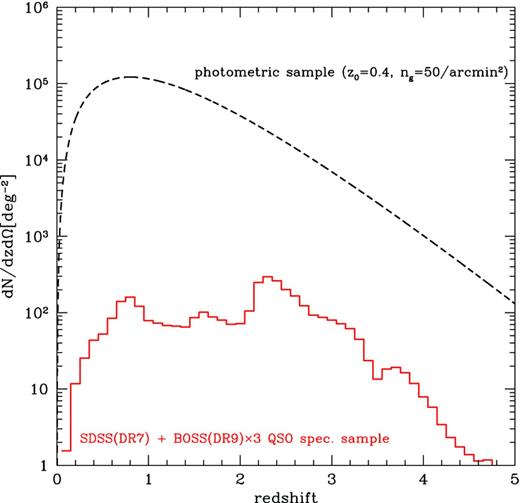
The histogram shows the redshift distribution of the spectroscopic quasar sample of SDSS DR7 (Schneider et al. 2010) and BOSS DR9 (Paris et al. 2012). The BOSS sample is multiplied by 3 as the DR9 has completed only the 1/3 of the target area. Dashed line shows the assumed photometric galaxy distribution, np(z) defined below equation (12), where we assumed |$\bar{n}_{\rm p}=50$| arcmin−2 for the total mean number density and 〈z〉 = 1.2 for the mean redshift.
RESULTS
Projected power spectrum
![Comparison of the projected and angular power spectrum at the mean redshift $\bar{z}=1.4$. Left: the angular autopower spectrum of photometric samples in the photo-z bins zp = [1.4 − Δz/2, 1.4 + Δz/2]. The thick and thin curves show the power spectrum for the bin width of Δzp ≃ 0.365 and 1.05, which corresponds to the width of the comoving radial distance, Δr = 0.5 and 1.5 Gpc h−1, respectively. The solid and dashed curves are the spectra assuming the photo-z accuracies of σz/(1 + z) = 0.05 or 0.3, receptively. Each thin dotted lines show the shot noise level for the photometric samples, which typically have the projected number density more than 104 deg−2 for an imaging survey we are interested in. Middle: similar to the left-hand panel, but for the cross-power spectrum between the spectroscopic and photometric samples, as a function of the transverse comoving separation (equation 7), where the transverse mode k is rescaled to the multipole via the distance to the spectroscopic sample by l = kr(z = 1.4) for an illustrative purpose. The solid and dashed curves are for the photo-z accuracies of the photometric galaxies, as in the left-hand panel. The cross-correlation preserves the BAO wiggles compared to the left-hand panel. Right: the projected autopower spectrum for the spectroscopic samples. The figure shows that, for a spectroscopic survey with a small number density $\bar{n}_{\rm s}<10^{2}\,{\rm deg}^{-2}$, the BAO wiggles in the autospectrum are difficult to measure due to the significant shot noise.](https://oup.silverchair-cdn.com/oup/backfile/Content_public/Journal/mnras/433/1/10.1093_mnras_stt761/1/m_stt761fig3.jpeg?Expires=1750217045&Signature=kF-Vuih8lf693JWU6Flt0VsRCcVrZQ-g3Z6TpswV7UiywuaMMNBU~jg5S0bxxfUi8eUT11ut20AT93sBAOspIw-wQvfaZOzH7WhTer1tJKgARs6Y9yCuGmZmcW0wxwZne7qiSDe7ZQ4NSnhv5ybtCVO8qWHTBwnR6ASFAQMkDSTgZ97nFmHNA1c5oiOQn4hFKCrqjp0xKpqpCvxJryjgU7EnekfChu4Z8A2V-H43x8S9WtHJq~Rz3uwz0tD0d2dXwiFlUHCPlj~Ii2iy56GPX2rrBh8UxJsbMOy2xFsycDBxM-OjsK8sUZQf~oPt2qY1lHaXsY0fNoi2K-tVa1pLcw__&Key-Pair-Id=APKAIE5G5CRDK6RD3PGA)
Comparison of the projected and angular power spectrum at the mean redshift |$\bar{z}=1.4$|. Left: the angular autopower spectrum of photometric samples in the photo-z bins zp = [1.4 − Δz/2, 1.4 + Δz/2]. The thick and thin curves show the power spectrum for the bin width of Δzp ≃ 0.365 and 1.05, which corresponds to the width of the comoving radial distance, Δr = 0.5 and 1.5 Gpc h−1, respectively. The solid and dashed curves are the spectra assuming the photo-z accuracies of σz/(1 + z) = 0.05 or 0.3, receptively. Each thin dotted lines show the shot noise level for the photometric samples, which typically have the projected number density more than 104 deg−2 for an imaging survey we are interested in. Middle: similar to the left-hand panel, but for the cross-power spectrum between the spectroscopic and photometric samples, as a function of the transverse comoving separation (equation 7), where the transverse mode k is rescaled to the multipole via the distance to the spectroscopic sample by l = kr(z = 1.4) for an illustrative purpose. The solid and dashed curves are for the photo-z accuracies of the photometric galaxies, as in the left-hand panel. The cross-correlation preserves the BAO wiggles compared to the left-hand panel. Right: the projected autopower spectrum for the spectroscopic samples. The figure shows that, for a spectroscopic survey with a small number density |$\bar{n}_{\rm s}<10^{2}\,{\rm deg}^{-2}$|, the BAO wiggles in the autospectrum are difficult to measure due to the significant shot noise.
To be comprehensive, we also show the expected cross-correlation function in configuration space, w(R), instead of the power spectrum in Fig. 4. As in the power spectrum, the overall shape and the BAO feature are preserved in the R-average case, whereas the BAO peak is significant smeared in the angle-average.
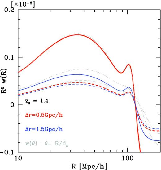
Similar to Fig. 3, but for the cross-correlation function in configuration space, w(R). As in Fig. 3, the top and dashed curves are the cross-correlation function assuming the photo-z errors of σz/(1 + z) = 0.05 and 0.3, respectively. The two curves differ for the redshift widths; the wider bin width changes only the amplitude of w(R), but preserve the overall shape and BAO feature. For comparison, the dotted lines show the angular cross-correlation w(θ = R/dA) for the same width of the (photometric) redshift bin; the BAO peak is significantly smeared.
Forecast for the cross-correlation BAO measurement
In this section, we study forecasts for the use of the projected power spectrum for measuring the BAO feature. In Fig. 5, we show the projected cross-power spectrum as a function of the transverse wavenumber, divided by the no-wiggle power spectrum (with the BAO feature being smoothed out), in order to highlight the BAO feature. Note that we used the transfer function in Eisenstein & Hu (1998) to compute the no-wiggle spectrum for the same cosmological model. Although we assume a linear galaxy bias multiplicative factor for both the spectroscopic (with bias parameter values based on those measured for SDSS quasars; Ross et al. 2009) and photometric samples (bp = 1.5), we include the effect of non-linear clustering on the matter power spectrum, using the publicly available code, regpt (Taruya et al. 2012), that includes up to the two-loop order contributions based on the refined perturbation theory. We show the cross-power spectra up to a certain maximum wavenumber, kmax, which is determined so that the non-linear matter power spectrum at the mean redshift is expected to be accurate to within a 1 per cent level accuracy in the amplitude compared to the simulation (Taruya et al. 2009, 2012). The figure clearly shows that the projected cross-power spectrum preserves the BAO feature, even for a wide redshift bin. On the other hand, the BAO feature is smeared in the angular correlation. We also notice that, for the higher redshift slice, the BAO feature remains up to the greater wavenumber due to the less evolving non-linearities.
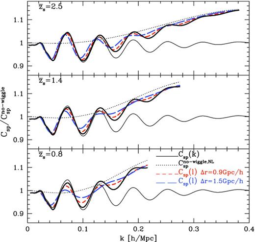
The projected power spectrum divided by the no-wiggle linear power spectrum in order to highlight the BAO feature, where we used Eisenstein & Hu (1998) to compute the no-wiggle spectrum. We consider |$\bar{z}_{\rm s}=2.5$| (top panel), 1.4 (middle) and 0.8 (bottom), respectively, for the mean redshift of the projection. The thick curves are the spectra computed when the non-linearity of the matter power spectrum is considered (see text for the details), while thin curves show the cross-power spectra in linear theory. The spectra are plotted up to kmax, where the non-linear power spectra are expected to be accurate to within 1 per cent at each mean redshift compared to simulations. For comparison, we also show the angular cross-power spectra projected over the redshift slice of Δr = 0.9 Gpc h−1 (short-dashed) and Δr = 1.5 Gpc h−1 (long-dashed) around each mean redshift, respectively, which are plotted against the wavenumber using the conversion |$kr(\bar{z})=l$|. The dotted curves are the non-linear power spectrum using the no-wiggle linear power spectrum for the input spectrum.
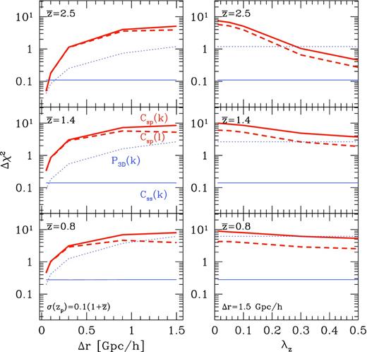
The expected significance of the BAO detection, Δχ2 (equation 17), for the cross-correlation analysis with different combinations of spectroscopic and photometric samples. We estimate the significance by comparing the cross-power spectra with and without the BAO wiggles, as in Fig. 5, but do not include the broad-band shape of the power spectrum. In each panel, the thick solid curves show the Δχ2 values for the projected cross-power spectrum (Csp(k)), the thick dashed curves are for the angular cross-power spectrum (Csp(l)) and the thin horizontal line is for the projected autocorrelation of the spectroscopic sample (Css(k)). For comparison, we also show the result when the BAO feature is extracted from the three-dimensional power spectrum analysis (P3D(k)), which is estimated using equation (18). The number density of the spectroscopic sample is fixed to (20Δz) deg−2, and the total number density of the photometric sample is assumed to |$\bar{n}_{\rm p}^{\rm tot} = 50\,{\rm arcmin}^{-2}$|. Results are shown for three mean redshift, |$\bar{z}_{\rm s}=2.5$| (top panels), 1.4 (middle) and 0.8 (bottom). Left: Δχ2 is calculated under the conditions that the photo-z accuracy is fixed to λz = 0.1 and the redshift bin width is varied from Δr = 0.1 to 1.5 Gpc h−1. Right: Δχ2 is calculated with a fixed redshift bin width Δr = 1.5 Gpc h−1, but with varying photo-z accuracies.
GEOMETRICAL TEST WITH THE CROSS-CORRELATION METHOD
In this section, we present more quantitative estimates on the power of the cross-correlation method for determining the angular diameter distance. For this forecast, in contrast to the preceding section, we include the broad-band shape information of the cross-power spectrum, extending the method in Seo & Eisenstein (2003) to a two-dimensional cross-correlation analysis. As a specific example, here we consider the cross-correlation BAO analysis assuming the SDSS/BOSS spectroscopic quasar catalogues (Schneider et al. 2010; Paris et al. 2012) as the spectroscopic sample (as shown in Fig. 2) and a mock photometric sample which has full overlap with the spectroscopic sample, as the photometric sample. We assume the total area of 10 000 deg2 for the overlapping area. We consider six redshift bins with the mean redshifts ranging from 0.7 to 2.9. The projected number density in each bin is estimated using the redshift distribution in Fig. 2. We use the bias parameters of the quasars in each redshift bin based on the measurement by Ross et al. (2009). For the photometric sample, we again assume the total number density of |$\bar{n}_{\rm p}^{\rm tot} = 50\,{\rm arcmin}^{-2}$|, and compute the number density in each redshift bin taking into account the photo-z error (see Section 2.1). Table 1 summarizes the set of the survey parameters.
A summary of survey parameters we consider for the forecast, and the expected fractional errors of determining the angular diameter distance, σ(DA)/DA, including marginalization over the other parameters. Here we consider the SDSS/BOSS spectroscopic quasar catalogue for the spectroscopic sample, and the Subaru HSC- or Euclid-type galaxy sample for the photometric sample. |$\bar{z_{\rm s}}$| and Δzs are the mean redshift and the redshift width for each redshift bin of the spectroscopic sample taken in the hypothetical cross-correlation analysis. bs, β and |$\bar{n}_{\rm s}$| are the linear bias, the linear RSD and the number density in each redshift bin (see text for the details). kmax is the maximum wavelength used for the Fisher matrix analysis. For each redshift bin, we cross-correlate the spectroscopic sample with the photometric galaxies based on their photo-zs assuming the photo-z errors of λz = 0.01, 0.1 and 0.3, respectively (see equation 16). np is the number density of the photometric galaxies in each redshift bin (see equation 12). The last column (|$\sigma _{D_{\rm A}}/D_{\rm A}$|) shows the expected error on the angular diameter distance measurement in each bin. For comparison, we also show the expected error when using the three-dimensional autopower spectrum of the spectroscopic sample (‘spec autocorrelation’).
| |$\bar{z_{\rm s}}$| | Δzs | bs | |$\beta (\bar{z_{\rm s}})$| | |$\bar{n}_{\rm s}$| (deg−2) | kmax (h Mpc−1) | Area (deg2) | λz | |$\bar{n}_{\rm p}$| (104 deg−2) | |$\sigma _{D_{\rm A}}/D_{\rm A}$| |
|---|---|---|---|---|---|---|---|---|---|
| 0.7 | 0.2 | 1.52 | 0.352 | 3 | 0.21 | 10 000 | 0.01 | 2.4 | 0.076 |
| 0.1 | 2.2 | 0.095 | |||||||
| 0.3 | 1.7 | 0.132 | |||||||
| Spec autocorrelation | 0.191 | ||||||||
| 0.9 | 0.2 | 1.70 | 0.333 | 3 | 0.23 | 10 000 | 0.01 | 2.4 | 0.095 |
| 0.1 | 2.3 | 0.095 | |||||||
| 0.3 | 1.7 | 0.137 | |||||||
| Spec autocorrelation | 0.237 | ||||||||
| 1.2 | 0.4 | 2.01 | 0.299 | 3.5 | 0.25 | 10 000 | 0.01 | 4.0 | 0.084 |
| 0.1 | 3.9 | 0.098 | |||||||
| 0.3 | 3.0 | 0.141 | |||||||
| Spec autocorrelation | 0.369 | ||||||||
| 1.6 | 0.4 | 2.49 | 0.252 | 3.5 | 0.29 | 10 000 | 0.01 | 2.7 | 0.080 |
| 0.1 | 2.7 | 0.103 | |||||||
| 0.3 | 2.4 | 0.188 | |||||||
| Spec autocorrelation | 0.475 | ||||||||
| 2.2 | 0.8 | 3.36 | 0.193 | 10 | 0.35 | 10 000 | 0.01 | 2.3 | 0.068 |
| 0.1 | 2.6 | 0.084 | |||||||
| 0.3 | 3.2 | 0.188 | |||||||
| Spec autocorrelation | 0.302 | ||||||||
| 2.9 | 0.6 | 4.60 | 0.144 | 10 | 0.42 | 10 000 | 0.01 | 0.5 | 0.075 |
| 0.1 | 0.6 | 0.133 | |||||||
| 0.3 | 1.4 | 0.536 | |||||||
| Spec autocorrelation | 0.306 | ||||||||
For comparison, we also show a forecast for using the three-dimensional power spectrum of the spectroscopic sample to estimate the cosmological distances, H(zi) and DA(zi). We follow the methods in Seo & Eisenstein (2007) (also see Ellis et al. 2012). We model the RSD (Kaiser 1987) and its non-linear effects (Eisenstein, Seo & White 2007) for the three-dimensional power spectrum with additional parameters; βi = dln D(zi)/dln a/bs and H(zi). The fiducial value of β is listed in Table 1. However, the results are not sensitive to the details, because the power spectrum information at relevant wavenumber bins is limited by the shot noise contamination for the sparse spectroscopic sample we are interested in.
Table 1 and Fig. 7 show an expected accuracy of the angular diameter distance measurement in each redshift bin via the cross-correlation method. The cross-correlation method allows for an improvement in the geometrical test compared to the three-dimensional autopower spectrum analysis, by reducing the shot noise contamination. For the SDSS/BOSS spectroscopic quasar catalogues, the cross-correlation method improves the fractional accuracy to better than 10 per cent in each redshift bin, if the photometric galaxy survey has a full overlap with the SDSS/BOSS footprints and if we can select adequate galaxy samples whose photo-z errors are better than λz = 0.1–0.2 (see equation 16). Also, an advantage of this method is to determine the angular diameter distance up to a high redshift of z ≃ 3, where the cosmic expansion is well in the decelerating expansion phase.
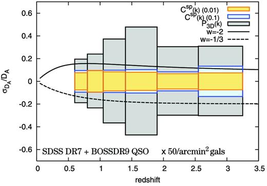
Expected accuracies on the angular diameter distance measurements with the cross-correlation BAO analysis as in Table 1. We show the results for the photo-z accuracies of both λz = 0.01 and 0.1, denoted as Csp(k)(0.01) or Csp(k)(0.1), respectively. The outermost boxes show the expected accuracies when the autocorrelation power spectrum of the spectroscopic quasar catalogue is used. The spectroscopic sample is divided into six subsamples with their spectroscopic redshifts. The solid and dashed curves show the changes in the angular diameter distance when the dark energy equation of state (w) is changed to −2 and −1/3 from w = −1 (the cosmological constant).
SUMMARY
In this paper, we have studied how the cross-correlation between a spectroscopic and a photometric sample can be used for the two-dimensional BAO measurement. We have shown that, with the aid of the spectroscopic sample, the cross-correlation preserves the BAO feature in the probed transverse scales, even for the projection over different redshifts such as Δz ≃ 1, while the angular (cross)-correlation suffers from a smearing of the BAO feature due to unavoidable photo-z errors that cause a mixing of the different physical scales in a particular angular scale (see Fig. 3). There are several notable advantages of this method. First, the cross-correlation significantly reduces the shot noise contamination in the measurement. Secondly, any statistical or systematic (catastrophic) photo-z errors affect only the overall normalization of the cross-correlation function, and do not change the shape of the power spectrum.
The cross-correlation method can be useful, if the spectroscopic sample has a wide coverage of redshift, but does not have a sufficiently high number density for the BAO measurement via the autocorrelation analysis. As a specific example, we have considered the SDSS/BOSS spectroscopic quasar sample to estimate the feasibility of the cross-correlation method, motivated by the fact that wide-area imaging surveys, such as the Subaru HSC Survey and Euclid, overlap with the SDSS/BOSS survey footprints. Here the SDSS/BOSS quasar sample has a wide redshift coverage of 0 < z ≲ 4 and wide area coverage of about 10 000 deg2, but has too small number density of ∼102 deg−2 per unit redshift interval to implement the BAO measurement via the autocorrelation analysis. On the other hand, the planned imaging surveys likely provide a much denser sampling of galaxies such as 103–105 deg−2 over the redshift range. We have shown that the cross-correlation allows a more accurate BAO measurement over 0.7 < z ≲ 3 than in the autocorrelation of the spectroscopic sample or the angular power spectrum of the photometric galaxies (see Figs 6 and 7 and Table 1), if the photometric redshift is reasonably good, 10–20 per cent level in the fractional accuracy, in order not to have a severe dilution in the measured cross-correlation. As shown in Fig. 7, the better photo-z accuracy of |$\sigma _z/(1+\bar{z}_{\rm s}) = 1$| per cent does not improve constraints on DA significantly compared to the 10 per cent photo-z accuracy. Hence the 10–20 per cent of the photo-z accuracy is sufficient for the cross-correlation BAO study, which can easily be achieved for the current and upcoming multiband photometric galaxy surveys.
The expected accuracy of the angular distance measurement in Fig. 7 is from both the BAO feature and the broad shape of the power spectrum. The projected cross-correlation allows us to measure the shape of the three-dimensional power spectrum (see equation 8), although the overall normalization is affected by photo-z errors. Hence, the method can also be used to constrain the tilt and running index of the primordial power spectrum. Also, as an ultimate possibility, the cross-correlation method may enable to use the observed radius of dark matter haloes in the projected distance. If we have a good knowledge on the virial radius of dark matter haloes as well as have a good estimator of halo masses, to observe the virial radius can be used to infer the angular diameter distance. This is relevant for cluster-shear weak lensing, which probes the halo and dark matter cross-correlation (Oguri & Takada 2011). Given that the clusters have follow-up spectroscopic redshifts, we can expect a high-precision measurement of the halo-matter cross-correlation at small scales down to a few Mpc, which correspond to the virial radii of massive haloes. Thus the virial radius may serve as another standard ruler that can lead to even higher precision measurements of the angular diameter distances. This is an interesting possibility and may worth exploring further.
We note that the cross-correlation technique developed in this paper can also be used to constrain the primordial non-Gaussianity via measurements of the largest scale cross-power spectra (Dalal et al. 2008; McDonald 2008; Slosar et al. 2008; Taruya, Koyama & Matsubara 2008). Again, by measuring the cross-correlation as a function of the transverse comoving separation, we can avoid the smearing effect due to the projection which reduces the enhanced power at the largest scales of k ≲ 0.01 h Mpc−1.
Spectroscopic observations of quasars, or more generally bright, rare galaxies, are relatively inexpensive in terms of the observation time needed for a given telescope. Such objects are also very interesting subjects for astronomical studies. The method developed in this paper can add a cosmological science case when combined with wide-area imaging surveys that have an overlap with the spectroscopic survey. The method is useful when designing joint spectroscopic and photometric surveys including a science case of the two-dimensional BAO analysis.
We thank Chiaki Hikage for useful discussion and valuable comments. We are grateful to the Atsushi Taruya for the use of publicly available regptfast code. This work is supported in part by the FIRST program ‘Subaru Measurements of Images and Redshifts (SuMIRe)’, CSTP, Japan, World Premier International Research Center Initiative (WPI Initiative), MEXT, Japan, JSPS Core-to-Core Program ‘International Research Network for Dark Energy’, by Grant-in-Aid for Scientific Research on Priority Areas No. 467 ‘Probing the Dark Energy through an Extremely Wide & Deep Survey with Subaru Telescope’ and by Grant-in-Aid for Scientific Research from the JSPS Promotion of Science (23740161 and 23340061).
In the flat-sky approximation, the unit vector is expanded around the North Pole as |$\boldsymbol {\gamma }\simeq (\vartheta \cos \varphi ,\vartheta \sin \varphi ,1)$|, and the two-dimensional flat-space vector can be defined as |$\boldsymbol {\theta }\equiv (\vartheta \cos \varphi ,\vartheta \sin \varphi )$|.
Suppose that the spectroscopic and photometric samples reside in their host haloes, which have the number densities of nh1 and nh2, and assume that some fractions of the two samples have the common host haloes which have the number density of nc. In this case, the shot noise for the cross-power spectrum is found to be proportional to nc/(nh1nh2).
