


Abstract
Using a compilation of 379 massive (stellar mass M ≳ 1011 M⊙) spheroid-like galaxies from the near-infrared Palomar/DEEP-2 survey, we investigated, up to z ∼ 1, whether the presence of companions depends on the size of the host galaxy. We explored the presence of companions for mass ratios with respect to the central massive galaxy down to 1 : 10 and 1 : 100, and within projected distances of 30, 50 and 100 kpc of these objects. We found evidence that these companions are equally distributed around both compact and extended massive spheroid-like galaxies. This suggests that, at least since z ∼ 1, the merger activity in these objects is nearly homogeneous across the whole population and that the merger history is not affected by the size of the host galaxy. Our results could indicate that compact and extended massive spheroid-like galaxies are increasing in size at the same rate.
INTRODUCTION
For a given stellar mass, the size of low-redshift massive early-type galaxies (stellar mass M ≳ 1011 M⊙) is found to be a factor of two larger than that of their counterparts at z ∼ 1 (e.g. Trujillo et al. 2004; McIntosh et al. 2005; Trujillo et al. 2006, 2007; Buitrago et al. 2008; Newman et al. 2012). In addition, the number density of such compact massive galaxies has decreased since that redshift (Cassata et al. 2011), with compact galaxies being extremely rare in the local Universe (Trujillo et al. 2009; Taylor et al. 2010) and having young ages (1–2 Gyr, Trujillo et al. 2009; Trujillo, Carrasco & Ferré-Mateu 2012; Ferré-Mateu et al. 2012), meaning that they cannot be the relics of compact high-redshift galaxies. How have compact massive galaxies evolved in size to occupy the present-day distribution? Now that it has been shown that major merging cannot be the only mechanism responsible for making galaxies increase in size since that epoch (e.g. López-Sanjuan et al. 2012), two alternative ideas have been suggested: the puffing-up model (Fan et al. 2008, 2010; Damjanov et al. 2009) and the minor merging scenario (Naab, Johansson & Ostriker 2009; Hopkins et al. 2009; Quilis & Trujillo 2012).
In the puffing-up model, galaxies increase in size through the removal of enormous quantities of gas by means of active galactic nuclei or supernova explosions during the early stages of the formation of spheroidal galaxies. Based on the analysis of stellar populations of local and high-redshift spheroidal galaxies, Trujillo, Ferreras & de La Rosa (2011) concluded that the evolution in size is independent of stellar age. This has been one of the main arguments against the puffing-up scenario. In the minor merging model, the size evolution observed in the massive spheroid-like galaxy population is caused mainly by the continuous bombardment of smaller pieces onto the main objects. Recent studies have tried to quantify the impact of the observed merger rates on the increase in size of massive galaxies (López-Sanjuan et al. 2012; Newman et al. 2012; Bluck et al. 2012). These studies focus on the evolution of the average size–mass relation. To progress these studies further, not only the average, but also the intrinsic dispersion of the size–mass relation should be examined with respect to the observed merger histories. Observations find a nearly constant, even decreasing, dispersion since z ∼ 1.5 (Trujillo et al. 2007; Cassata et al. 2011; Newman et al. 2012), while cosmological simulations suggest that merging tends to increase the dispersion of the size–mass relation with cosmic time (e.g. Nipoti et al. 2012). A fundamental ingredient in such comparisons of models versus observation is the variation of the merger rate with size at a given stellar mass; for example, if compact galaxies have higher merger activity, they will evolve faster across the size–mass relation. In this paper we explore whether merging occurs for all galaxies of a given stellar mass with the same probability, or whether it is more frequent for galaxies with smaller sizes, which are quite rare in the local Universe compared with compact ones at higher redshifts. Answering this question is crucial to understanding how the local stellar mass–size relation developed.
As a proxy for measuring the minor merging activity in massive spheroidal galaxies since z ∼ 1 we study the frequency of companions around massive galaxies since that epoch. We assume that these companions will eventually be accreted onto the main galaxy. In particular, we study whether the companions are preferentially located around galaxies with a specific size in the stellar size–mass relation or whether they are homogeneously distributed among the galaxy population independently of their stellar mass and size. We focused our analysis on redshifts up to z ∼ 1. This is approximately the redshift at which our data, presented in Mármol-Queraltó et al. (2012, hereafter MQ12), allow us to explore with completeness the presence of companions around our sample of massive (stellar mass M ≳ 1011 M⊙) galaxies, for stellar mass ratios between the central massive galaxy (Mcentral) and its companion (Mcom) down to 0.01 < Mcom/Mcentral < 1 (1 : 100).
This paper is organized as follows. In Section 2 we present the two samples used in this work: the sample of central massive spheroid-like galaxies, with a brief description of the Palomar/DEEP-2 survey; and the sample of companions, from the Rainbow Database, around them. We explain the companion detection process in Section 3. We present the analysis of the data in Section 4, together with the contamination corrections arising from uncertainties in the photometric redshifts. Finally, in Section 5, we present the conclusions of our findings and a brief summary. In this paper we adopt a standard ΛCDM cosmology, with Ωm = 0.3, ΩΛ = 0.7, H0 = 100h km s−1 Mpc−1 and h = 0.7.
THE DATA
To study whether the size of the massive spheroid-like galaxies is relevant for their merger history, we use a complete, mass-selected, large catalogue of massive galaxies. We explore which of these objects have companions that would be able to merge with the central massive galaxy. Thus, our analysis is based on two data sets: a catalogue with central massive spheroid-like galaxies and another sample containing their companion galaxies.
As the reference catalogue for the central massive spheroid-like galaxies we used the compilation of Trujillo et al. (2007, hereafter T07). The Ks-band imaging from the Palomar Observatory Wide-field Infrared (POWIR)/DEEP-2 survey (Davis et al. 2003; Bundy et al. 2006; Conselice et al. 2007) was used to define a sample of 831 massive galaxies (stellar mass M > 1011M⊙) up to z = 2 located over ∼710 arcmin2 in the Extended Groth Strip (EGS). In addition, these objects were imaged with the Advanced Camera for Surveys (ACS) from the Hubble Space Telescope (HST) in the F606W and F814W bands, with the CFH12K camera from the Canada–France–Hawaii Telescope in the B, R and I bands, and with the Palomar 5-m telescope in the J and Ks bands. T07 present massive galaxies with spectroscopic redshifts that have been supplemented with photometric redshifts with an accuracy of Δz/(1 + z) ∼ 0.07. Stellar masses were estimated using a Chabrier (2003) initial mass function. T07 estimated the circularized half-light radius (re) and Sérsic indices n (Sèrsic 1968) for all galaxies in the central sample. The criterion used to identify the massive spheroid-like objects is based on the Sérsic indices. The Sérsic index can be used to make a reliable morphological classification of galaxies, as it measures the shape of the surface brightness profile (Andredakis, Peletier & Balcells 1995). In order to obtain a reliable sample of bulge-dominated galaxies and to exclude late-type galaxies with a bright nucleus, we selected the galaxies that have Sérsic indices larger than 2.5 (see fig. 1 in Ravindranath et al. 2004).
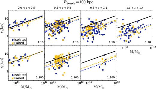
Stellar size–mass relation of spheroid-like galaxies in various redshift bins. The different panels show the distribution of paired (yellow crosses) and isolated (blue dots) galaxies down to mass ratios of 1 : 10 (upper panels) and 1 : 100 (lower panels), in all cases within a projected distance of 100 kpc. The black line represents the local stellar size–mass relation (Shen et al. 2003) for spheroid-like galaxies. For every redshift bin, the dashed yellow and blue lines show the best fits to the distribution of paired and isolated galaxies, respectively (see Section 4 for more details).
To compile the sample of companion galaxies around our massive spheroid-like objects we used the EGS IRAC-selected galaxy sample from the Rainbow Cosmological Database1 published by Barro et al. (2011a, see also Pérez-González et al. 2008). This data base provides spectral energy distributions (SEDs) ranging from the UV to the mid-infrared, plus well-calibrated and reliable photometric redshifts and stellar masses (Barro et al. 2011b). In general, the companions sampled have photometric redshifts from the Rainbow Database. We refer to this resulting sample as the Rainbow catalogue.
In order to build a sample of central massive galaxies with the best estimates of redshifts and stellar masses we followed the same criterion as in MQ12: if a given central galaxy has a spectroscopic redshift in the Rainbow catalogue, both the redshift and the stellar mass are taken from this catalogue. Otherwise, spectroscopic redshifts and stellar masses are taken from T07. If the central galaxy has no spectroscopic redshift in either of the two above data sets, we take the Rainbow photometric redshift as long as it is in agreement with the photometric redshift of T07. More precisely, we impose that the condition that the difference between the photometric redshifts in the two catalogues has to be smaller than 0.070 at 0.0 < z < 0.5, than 0.061 at 0.5 < z < 1.0, and than 0.083 at z > 1.0. When a larger difference is found, the central galaxy is rejected for this study.
To ensure that the fraction of galaxies with companions along our explored redshift range is not biased by the stellar mass completeness limit of the Rainbow catalogue, we keep in the central sample only those galaxies that are at least 10 (100) times more massive than the stellar mass limit of the companion sample at each redshift. The stellar mass limit (75 per cent complete) of the Rainbow catalogue at each redshift is provided in Pérez-González et al. (2008) and ranges from M ≳ 108.5 M⊙ at z ∼ 0.2 to M ≳ 1010 M⊙ at z ∼ 1.2 (see fig. 4 in Pérez-González et al. 2008). These stellar mass limits correspond to the stellar mass of a passively evolving galaxy formed in a single instantaneous burst of star formation that occurred at z ∼ ∞ and having a 3.6-μm flux equal to the 75 per cent completeness level in the IRAC galaxy sample ([3.6] ∼ 24.75 mAB). In the redshift range 0 < z < 1.4 we can probe companions with a mass fraction compared with their central objects (stellar mass M ≳ 1011 M⊙) down to 1 : 10. There are finally 379 massive spheroid-like galaxies that meet all the above criteria, out of which 239 have spectroscopic redshifts and 140 have photometric redshifts. In the redshift range 0 < z < 1.1 we are able to explore the presence of companions down to a mass ratio of 1 : 100. The number of massive spheroid-like galaxies for which this study can be conducted is 145 (107 with spectroscopic redshifts and 38 with photometric redshifts).
DETECTION OF COMPANIONS
The process and criteria used to search for companions around massive spheroid-like galaxies is based on MQ12. A galaxy from the Rainbow catalogue is considered as a potential companion if the redshift difference between the object and the central host is less than the 1σ uncertainty, within a projected radial distance Rsearch around the central object. Usual values of Rsearch in the literature range from 30 to 150 kpc in our reference cosmology (h = 0.7, e.g. Patton et al. 2000; Bell et al. 2006; Mármol-Queraltó et al. 2012; Bluck et al. 2012). With these Rsearch values, the selected pairs will merge on a relatively short time-scale (t ≲ 2.5 Gyr, Lotz et al. 2010). In the following we explore three search radii, namely Rsearch = 30, 50 and 100 kpc. Larger search radii increase the background contamination, and the results become very uncertain. Finally, we consider only those companion objects within a mass range of 0.1 < Mcom/Mcentral < 1 if we explore our sample up to z = 1.4, and those within 0.01 < Mcom/Mcentral < 1 if the analysis is constrained to massive galaxies with z < 1.1. Hereafter, we refer to massive spheroid-like galaxies with companions as paired galaxies, and to massive spheroid-like galaxies without companions as isolated galaxies. These concepts are defined specifically for this work, so the definitions may differ from those of other publications.
It is clear that the main source of contamination in this sort of study comes from the uncertainties in the photometric redshifts. Owing to the background/foreground contamination, there exists a fraction of fake paired galaxies with this method of companion detection (see Section 4.1.1). In addition, there also exists a fraction of fake isolated galaxies, given that the redshift difference between the host galaxy and the potential candidate is set to be within a 1σ uncertainty (see Section 4.1.2). Note that these two effects can be constrained and corrected only by statistical methods. Because the study in this paper is performed over individual galaxies and it is not possible to state whether the companion of a particular massive central galaxy is real or a contaminant, we devote Section 4.1.3 to probing in detail the impact of these two effects on our results, as well as to accounting for them statistically by means of Monte Carlo simulations.
ANALYSIS OF THE DATA
The main goal of the present work is to address whether the presence of companions, with mass ratios down to 1 : 10 and 1 : 100, depends on the size of massive spheroid-like galaxies. We split our sample into distinct redshift bins in order to analyse the cosmic time evolution of this dependence. In Figs 1, 2 and 3 we show the stellar size–mass relation of our sample of central massive spheroidal-like galaxies for various redshift bins and search radii Rsearch = 30, 50 and 100 kpc, according to the criteria described in Section 3. It is clear that these plots suggest that the paired galaxies are distributed homogeneously through the stellar size–mass relation at all redshifts, independently of whether the existence of companions in the 1 : 10 or in the 1 : 100 mass ratio range is being considered. We now quantify this in more detail.
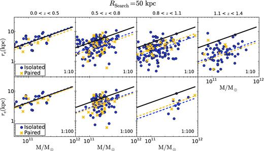
As Fig. 1, but using a search radius of 50 kpc for the companion detection process (see Section 3).
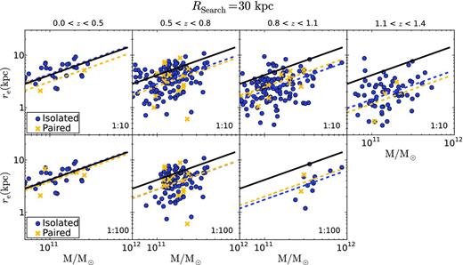
As Fig. 1, but using a search radius of 30 kpc for the companion detection process (see Section 3).
The best-fitting parameter b (see equation 1) of the stellar size–mass distribution for paired and isolated galaxies as a function of redshift, search radius and mass ratio.
| Parameter b [10−6 kpc] | |||||||
|---|---|---|---|---|---|---|---|
| Mass ratio 1 : 10 | Rsearch = 30 kpc | Rsearch = 50 kpc | Rsearch = 100 kpc | ||||
| Redshift | bpair | biso | bpair | biso | bpair | biso | Global |
| 0.0 < z < 0.5 | 2.15 ± 0.58 | 3.01 ± 0.28 | 2.45 ± 0.46 | 3.04 ± 0.29 | 2.47 ± 0.43 | 3.06 ± 0.30 | 2.90 ± 0.25 |
| 0.5 < z < 0.8 | 1.76 ± 0.20 | 1.96 ± 0.08 | 1.70 ± 0.16 | 1.98 ± 0.08 | 2.08 ± 0.14 | 1.87 ± 0.09 | 1.93 ± 0.07 |
| 0.8 < z < 1.1 | 1.71 ± 0.23 | 1.43 ± 0.06 | 1.74 ± 0.17 | 1.40 ± 0.06 | 1.64 ± 0.11 | 1.37 ± 0.06 | 1.45 ± 0.05 |
| 1.1 < z < 1.4 | 0.82 ± 0.22 | 0.99 ± 0.06 | 0.87 ± 0.15 | 0.99 ± 0.06 | 0.86 ± 0.11 | 1.01 ± 0.06 | 0.98 ± 0.05 |
| Mass ratio 1 : 100 | Rsearch = 30 kpc | Rsearch = 50 kpc | Rsearch = 100 kpc | ||||
| Redshift | bpair | biso | bpair | biso | bpair | biso | Global |
| 0.0 < z < 0.5 | 2.65 ± 0.55 | 2.96 ± 0.28 | 2.71 ± 0.47 | 2.97 ± 0.29 | 2.89 ± 0.42 | 2.91 ± 0.31 | 2.90 ± 0.25 |
| 0.5 < z < 0.8 | 1.91 ± 0.24 | 1.89 ± 0.09 | 1.79 ± 0.15 | 1.94 ± 0.10 | 2.04 ± 0.12 | 1.68 ± 0.12 | 1.90 ± 0.09 |
| 0.8 < z < 1.1 | 1.39 ± 0.46 | 1.21 ± 0.17 | 1.42 ± 0.38 | 1.18 ± 0.17 | 1.41 ± 0.25 | 1.05 ± 0.20 | 1.23 ± 0.16 |
To confirm the above result we performed Kolmogorov–Smirnov and t-Student tests for the distributions of paired and isolated galaxies in the size–mass plane. To do that, we performed the fitting of equation (1) to the whole central galaxy sample (see the global parameters in Table 1) for every redshift and mass range, and studied the distances to this relation for the paired and isolated galaxy populations. In Table 2 we show the Kolmogorov–Smirnov and t-Student estimators obtained for our sample of central massive galaxies, denoted EKS and ETS respectively, as well as their limiting values for confidence levels of 95 per cent of the two distributions, taking into account the degrees of freedom of each subsample. In all cases the estimators are smaller than the limiting values, and consequently we infer that the two distributions are statistically indistinguishable at the 95 per cent confidence level. This implies that the size–mass distributions of paired and isolated galaxies are not statistically different.
Test estimators obtained for the Kolmogorov–Smirnov and t-Student tests, denoted by EKS and ETS respectively. We present the values of the estimators for a confidence level of 95 per cent, denoted by EKS(95 per cent) and ETS(95 per cent), taking into account the degrees of freedom of each subsample.
| Test estimators | ||||||||
|---|---|---|---|---|---|---|---|---|
| Mass ratio 1 : 10 | Mass ratio 1 : 100 | |||||||
| Kolmogorov–Smirnov | t-Student | Kolmogorov–Smirnov | t-Student | |||||
| Redshift | EKS | EKS(95 per cent) | ETS | ETS(95 per cent) | EKS | EKS(95 per cent) | ETS | ETS(95 per cent) |
| Rsearch = 30 kpc | ||||||||
| 0.0 < z < 0.5 | 0.538 | 0.720 | 1.502 | 2.052 | 0.342 | 0.602 | 0.588 | 2.052 |
| 0.5 < z < 0.8 | 0.176 | 0.344 | 0.715 | 1.977 | 0.203 | 0.372 | 0.069 | 1.984 |
| 0.8 < z < 1.1 | 0.204 | 0.386 | 0.957 | 1.977 | 0.409 | 0.864 | 0.359 | 2.201 |
| 1.1 < z < 1.4 | 0.270 | 0.712 | 0.444 | 1.998 | ||||
| Rsearch = 50 kpc | ||||||||
| 0.0 < z < 0.5 | 0.408 | 0.569 | 1.284 | 2.052 | 0.298 | 0.538 | 0.550 | 2.052 |
| 0.5 < z < 0.8 | 0.189 | 0.293 | 1.261 | 1.977 | 0.176 | 0.291 | 0.649 | 1.984 |
| 0.8 < z < 1.1 | 0.289 | 0.308 | 1.467 | 1.977 | 0.300 | 0.749 | 0.563 | 2.201 |
| 1.1 < z < 1.4 | 0.334 | 0.505 | 0.458 | 1.998 | ||||
| Rsearch = 100 kpc | ||||||||
| 0.0 < z < 0.5 | 0.448 | 0.538 | 1.346 | 2.052 | 0.184 | 0.486 | 0.045 | 2.052 |
| 0.5 < z < 0.8 | 0.172 | 0.235 | 1.036 | 1.977 | 0.228 | 0.262 | 1.773 | 1.984 |
| 0.8 < z < 1.1 | 0.184 | 0.235 | 1.632 | 1.977 | 0.524 | 0.675 | 1.133 | 2.201 |
| 1.1 < z < 1.4 | 0.235 | 0.393 | 0.742 | 1.998 | ||||
The most representative search radius for this study is 50 kpc, as both the background/foreground contamination and the detection contamination are fairly low (∼10 per cent in both cases), and the number of paired galaxies ensures good statistics. For a search radius of 50 kpc, Fig. 4 illustrates that the ratio between the b-parameters of both populations (paired and isolated galaxies) is consistent with unity within the errors, implying that there is no significant shift between the two distributions. Fig. 5 gives the histograms of the distances of paired (yellow) and isolated (blue) galaxies to the fitting of the size–mass relation (equation 1) of the whole central galaxy sample for a search radius of 50 kpc. Dashed yellow and blue lines show the mean values of the paired and isolated distributions, respectively. For a t-Student test, the shadow area is the difference between the mean values of the two distributions for a confidence level of 95 per cent with the same degrees of freedom. In all cases, the means of the two populations are statistically the same for a confidence level of 95 per cent in the t-Student test. Fig. 6 shows the cumulative distribution function (CDF) of the histograms in Fig. 5. The vertical red line is the largest difference between the CDFs of the paired and isolated galaxies. For a Kolgomorov–Smirnov test, the shadow area is the difference between the CDFs of the two distributions for a confidence level of 95 per cent with the same degrees of freedom. In every panel, the red line is smaller than the shadow area, so the two distributions (paired and isolated) are statistically the same in the Kolmogorov–Smirnov test. We obtained similar results for the search radii Rsearch = 30 and 100 kpc.
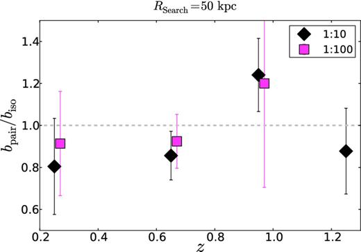
The ratio of the b-parameters of the size–mass relation (equation 1) for paired and isolated massive central galaxies in various redshift bins for two mass ratios (1 : 10, black diamonds; 1 : 100, pink squares). The figure shows the case of a search radius of 50 kpc. A ratio close to 1 implies that the average sizes of paired and isolated massive galaxies are the same.
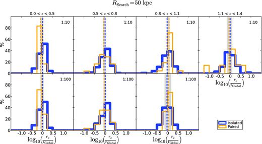
Histograms of the distances of paired (yellow) and isolated (blue) galaxies to the size–mass relation (equation 1) for the whole central galaxy sample, using a search radius of 50 kpc and mass ratios of 1 : 10 (upper panels) and 1 : 100 (lower panels). Dashed yellow and blue lines show the mean values of the paired and isolated distributions, respectively. The shadow area is the difference between the means of two distributions for a confidence level of 95 per cent with the same degrees of freedom for a t-Student test. In all cases, the means of the two populations are statistically the same.
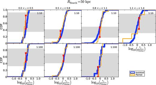
Cumulative distribution functions (CDFs) of the distances of paired (yellow) and isolated (blue) galaxies to the size–mass relation (equation 1) for the whole central galaxy sample, using a search radius of 50 kpc and mass ratios of 1 : 10 (upper panels) and 1 : 100 (lower panels). The red lines illustrate the largest distance between the CDFs of paired and isolated galaxies. The shadow area is the difference between the CDFs of two distributions for a confidence level of 95 per cent with the same degrees of freedom for a Kolmogorov–Smirnov test. In all cases, the shifts between the CDFs are statistically compatible.
Systematic effect analysis
These results were obtained by comparing the distributions of paired and isolated galaxies, but neither the background/foreground contamination nor the fake isolated galaxy contamination were taken into account, as we cannot correct for these effects individually. The two effects are studied in Sections 4.1.1 and 4.1.2, respectively. Finally, Section 4.1.3 is devoted to checking the impact of these contamination sources on our results.
Background/foreground contamination correction
For the method of companion detection described in Section 3, MQ12 showed that there exists an excess in the number of paired galaxies owing to the photometric redshift uncertainties (background/foreground contamination). Because we could be considering some galaxies to be companions when they are not really linked gravitationally to the host galaxy, leading to fake paired galaxies, such redshift uncertainties are the main source of contamination. Consequently, it is necessary to estimate statistically the background/foreground contamination and to check to what extent our results may be affected.
We followed the statistical process in MQ12 to estimate the background/foreground contamination. This method consists of placing mock massive galaxies randomly in the volume of the Rainbow catalogue. The number of mock galaxies in every redshift bin is the same as in our observed sample, and the mock galaxy parameters are the same as the massive spheroid-like galaxy parameters, for example for redshift and stellar mass. Once the mock galaxies are situated in the Rainbow catalogue volume, we apply the companion detection process explained above (including the 1σ uncertainty in the estimation of the redshifts) and compute the fraction of these mock galaxies having companions, Fpair, mock, around them for search radii Rsearch = 30, 50 and 100 kpc, for the mass ratios 1 : 10 and 1 : 100. To obtain a robust count of the paired mock galaxies, we repeat this process 100,000 times. We reasonably assume that the average fraction of paired mock galaxies, |$\overline{F}_{\rm pair,mock}$|, corresponds to the fraction of galaxies affected by the background/foreground contamination.
The simulation results, shown in Table 3, indicate that up to ∼4, 9 and 24 per cent (∼6, 14 and 26 per cent) of the observed paired galaxies in the mass ratio 1 : 10 (1 : 100) actually have no companions within a search radius of 30, 50 and 100 kpc.
Bias in the determination of paired and isolated galaxies attributable to the photometric redshift uncertainties. For each redshift range we present the number of massive galaxies Ncentral, the observed fraction of paired massive galaxies Fpair, obs, and the fraction of paired galaxies after the contamination correction Fpair, with their errors. We show the overestimation in the number of paired galaxies attributable to the redshift uncertainties with this method of companion detection Cpair. We also present the fraction of fake isolated galaxies, Ciso, attributable to the assumption of a 1σ uncertainty criterion.
| Mass ratio 1 : 10 | Mass ratio 1 : 100 | ||||||||||
|---|---|---|---|---|---|---|---|---|---|---|---|
| Redshift range | Ncentral | Fpair, obs | Fpair | Cpair | Ciso | Ncentral | Fpair, obs | Fpair | Cpair | Ciso | |
| Rsearch = 30 kpc | |||||||||||
| 0.0 < z < 0.5 | 29 | 0.100 | 0.097 ± 0.010 | 0.03 | 0.05 | 29 | 0.200 | 0.192 ± 0.019 | 0.04 | 0.10 | |
| 0.5 < z < 0.8 | 142 | 0.113 | 0.110 ± 0.005 | 0.03 | 0.05 | 103 | 0.136 | 0.127 ± 0.010 | 0.07 | 0.06 | |
| 0.8 < z < 1.1 | 142 | 0.085 | 0.082 ± 0.004 | 0.04 | 0.04 | 13 | 0.154 | 0.147 ± 0.026 | 0.05 | 0.07 | |
| 1.1 < z < 1.4 | 66 | 0.045 | 0.042 ± 0.006 | 0.07 | 0.02 | ||||||
| Rsearch = 50 kpc | |||||||||||
| 0.2 < z < 0.5 | 29 | 0.20 | 0.19 ± 0.02 | 0.06 | 0.10 | 29 | 0.27 | 0.23 ± 0.04 | 0.13 | 0.14 | |
| 0.5 < z < 0.8 | 142 | 0.17 | 0.16 ± 0.01 | 0.09 | 0.08 | 103 | 0.27 | 0.23 ± 0.02 | 0.14 | 0.14 | |
| 0.8 < z < 1.1 | 142 | 0.15 | 0.14 ± 0.01 | 0.08 | 0.07 | 13 | 0.23 | 0.20 ± 0.06 | 0.14 | 0.11 | |
| 1.1 < z < 1.4 | 66 | 0.11 | 0.09 ± 0.01 | 0.12 | 0.04 | ||||||
| Rsearch = 100 kpc | |||||||||||
| 0.0 < z < 0.5 | 29 | 0.23 | 0.18 ± 0.05 | 0.24 | 0.10 | 29 | 0.37 | 0.20 ± 0.08 | 0.45 | 0.14 | |
| 0.5 < z < 0.8 | 142 | 0.32 | 0.25 ± 0.03 | 0.23 | 0.15 | 103 | 0.62 | 0.50 ± 0.04 | 0.20 | 0.56 | |
| 0.8 < z < 1.1 | 142 | 0.32 | 0.26 ± 0.02 | 0.19 | 0.16 | 13 | 0.54 | 0.41 ± 0.12 | 0.24 | 0.38 | |
| 1.1 < z < 1.4 | 66 | 0.20 | 0.12 ± 0.03 | 0.38 | 0.17 | ||||||
Fake isolated galaxies due to the 1σ uncertainty condition
In the companion detection process, the candidates were constrained to have a difference in redshift from the central massive galaxy that is lower than the 1σ uncertainty. Assuming that both the central galaxy and its companion have photometric redshifts, we expect to miss Fσ ∼ 30 per cent of the companions in our search. MQ12 estimated that allowing for a difference of up to 2σ, instead of 1σ, in the search of companions, the background/foreground contamination effects increase by ∼50 per cent, whereas the fraction of paired galaxies changes by less than 30 per cent, as expected. Thus, the 1σ condition is the optimal one for merger fraction studies, as shown by MQ12.
Because Fσ ∼ 30 per cent, we estimate that Ciso (see Table 3) is lower than 4, 7 and 14 per cent (7, 14 and 46 per cent) for search radii of 30, 50 and 100 kpc for the mass ratio 1 : 10 (1 : 100).
Reliability of results
Owing to the photometric redshift uncertainties, we must check whether the contamination in the companion detection can affect our results. Because we cannot correct for the contamination of central galaxies individually, we adopt a statistical Monte Carlo approach, as a sanity check, to ensure that the background/foreground contamination and the 1σ assumption are not compromising our results. First, we randomly move central paired galaxies from the observed sample to the isolated sample, to reach the expected number of fake paired galaxies after the contamination correction according to Table 3. Second, we randomly move observed isolated galaxies to the set of paired galaxies, independently of their sizes or masses, until the expected numbers of fake isolated galaxies presented in Table 3 are recovered. Because the errors in the detection of companions are fully linked to the errors in the determination of the redshifts, we can reasonably assume that the fake paired and fake isolated galaxies will be randomly located around the size–mass relation, independently of the mass or size. We then apply Kolmogorov–Smirnov and t-Student tests over the new samples of paired and isolated galaxies. We repeat this process one million times and determine the fraction of cases for which the two distributions are undistinguishable, according to the above statistical tests.
According to these tests, we obtain that for the vast majority of iterations ( ≳ 96 per cent) the size–mass distributions of paired and isolated massive central galaxies cannot be statistically distinguished. We therefore conclude that the potential contaminants described in this section do not compromise the findings of this work.
SUMMARY AND CONCLUSIONS
Using a compilation of 379 massive (stellar mass M ≳ 1011 M⊙) spheroid-like galaxies from the near-infrared Palomar/DEEP-2 survey, we have demonstrated that, at least since z ∼ 1, there are no significant differences between the distributions of massive spheroid-like galaxies with (paired) and without (isolated) companions over the size–mass plane. We found that the probability of finding companions around the host galaxy is independent of its size at a given mass, as the companions are not located preferentially around the more compact or extensive massive spheroid-like galaxies. Our finding is independent of the search radius, the redshift and the mass ratio between the spheroid-like massive central galaxy and its companion.
We explored the size–mass relation for the population of paired and isolated massive spheroid-like galaxies at various redshifts, keeping its slope constant and equal to that obtained by Shen et al. (2003) in the local Universe. We analysed the shift between the offsets of the size–mass relation of the paired and isolated populations, finding that they are compatible within errors in every case. We also performed two statistical tests, Kolmogorov–Smirnov and t-Student, over both populations to confirm that there are no significant differences between them. Given the methodology for identifying companions, the uncertainty in the redshift produces a contamination in the fraction of paired galaxies. This uncertainty is independent of the host galaxy position over the size–mass plane, and thus we can correct for this effect statistically but not individually. We checked that this contaminant factor does not affect our findings through a Monte Carlo approach.
Our results suggest that, at least since z ∼ 1, the merger activity in massive spheroid-like galaxies is rather homogeneous across the whole population, and their merger history is not affected by the size of the host galaxy at a given stellar mass. This suggests that it is very likely that compact and extended spheroid-like massive galaxies are increasing in size at the same rate. Future studies confronting the observed merger history of massive galaxies with the evolution of the size–mass relation, regarding both its median and intrinsic dispersion, will benefit from the observational constraints presented in this work.
The authors acknowledge the referee's comments, which led to improvements in this work. They also thank Carlos Hernández-Monteagudo for his very useful advice. LADG acknowledges support from the ‘Caja Rural de Teruel’ to develop this research. AJC is a Ramón y Cajal Fellow of the Spanish Ministry of Economy and Competitiveness. This work was supported by the ‘Programa Nacional de Astronomía y Astrofísica’ of the Spanish Ministry of Economy and Competitiveness under grants AYA2012-30789, AYA2010-21322-C03-02, AYA2009-10368 and AYA2009-07723-E. This work made use of the Rainbow Cosmological Surveys Database, which is operated by the Universidad Complutense de Madrid (UCM).
