Void statistics and hierarchical scaling in the halo model

Fry, J. N.; Colombi, S.

doi:10.1093/mnras/stt745

Abstract

We study scaling behaviour of statistics of voids in the context of the halo model of non-linear large-scale structure. The halo model allows us to understand why the observed galaxy void probability obeys hierarchal scaling, even though the premise from which the scaling is derived is not satisfied. We argue that the commonly observed negative binomial scaling is not fundamental, but merely the result of the specific values of bias and number density for typical galaxies. The model implies quantitative relations between void statistics measured for two populations of galaxies, such as SDSS red and blue galaxies, and their number density and bias.

methods: numerical, methods: statistical, galaxies: statistics, large-scale structure of Universe

INTRODUCTION

Understanding the behaviour of voids in the galaxy distribution is one of the remaining unsolved problems of large-scale structure. Voids are a powerful probe of non-linear large-scale structure. They probe high-order statistical properties, but do so on scales that should be accessible in perturbation theory. One interesting property of voids is a scaling behaviour implied in the hierarchical model of higher order clustering. The hierarchical scaling has been verified many times, in a variety of samples, including the CfA redshift survey (Maurogordato & Lachièze-Rey 1987; Vogeley et al. 1994), Perseus-Pisces Fry et al. (1989), the Southern Sky Redshift Survey (Maurogordato, Schaeffer & da Costa 1992) and IRAS 1.2 Jy (Bouchet et al. 1993). Particularly intriguing are recent results from 2dFGRS (Croton et al. 2004a, 2007) and from DEEP2 and SDSS (Conroy et al. 2005; Tinker et al. 2008), in which the scaling continues to hold with improved precision over larger scales, for both magnitude selected subsamples and random dilutions.

However, in data (Bouchet et al. 1993; Gaztañaga 1994; Croton et al. 2004b; Ross, Brunner & Myers 2006, 2007), and in numerical simulations (Fry et al. 2011), the hierarchical clustering on which the scaling is based is not obeyed. The hierarchical normalization removes much of the variation, but the hierarchical amplitudes still depend on scale, and the premise of the scaling does not hold in detail. A recent alternative to purely hierarchical behaviour is provided by the halo model (Ma & Fry 2000a,b; Scoccimarro et al. 2001). In this paper, we show that void scaling can be understood in the halo model.

In Section 2, we review statistics and display the connection between voids and correlation functions, and we apply the halo model. Many common models are realizations of the halo model, and we present several of these in Section 3. In Section 4, we test the model against numerical results and present several halo model scaling relations. Section 5 contains a final discussion.

STATISTICS OF VOIDS

Generating functions

The probability that a volume be empty of galaxies, or void, is an intriguing statistical measure, accessible to perturbation theory on large scales and yet an inherently non-linear statistic on all scales. We study the properties of voids in the context of the halo model, the essence of which is that galaxies come in groups or clusters embedded in haloes; the number of galaxies is then the sum over haloes of the number within each halo. The generating function formulation of the halo model (Fry et al. 2011) is useful for studying combinatorics, and particularly voids. Let the probability and moment generating functions be

\begin{equation} G(z) = \sum _{n=1}^\infty P_n \, z^n = {{\left \langle z^n \right\rangle }} , \end{equation}

(1)

\begin{eqnarray} M(t) &=& \sum _{k=1}^\infty {1 \over k!} \, m_k \, t^k, \end{eqnarray}

(2)

where P_n is the probability that a randomly placed volume contains n galaxies, and m_k is the order k factorial moment of the distribution, |$m_k = {\bar{N}}^k \, {\bar{\mu }}_k = \mathop {{\langle }}\nolimits n^{[k]}\mathop {{\rangle }}\nolimits$|⁠, where n^[k] = n(n − 1) ⋅⋅⋅ (n − k + 1) = n!/(n − k)!. Since both probabilities and moments can be obtained as derivatives of G, probabilities as

\begin{equation} P_n = {1 \over n!} \, {{\rm d}^n \over {\rm d}z^n} G(t) \Bigr |_{z=0}, \end{equation}

(3)

and moments as

\begin{equation} m_k = {{\left \langle n (n-1) \cdots (n-k+1) \right \rangle = {{\rm d}^k \over {\rm d}z^k} G(z)}} \Bigr |_{z=1}, \end{equation}

(4)

we see that the generator M(t) of moments, so that |$m_k = {\rm d}^k M(t)/{\rm d}t^k |_{t=0}$| is thus M(t) = G(t + 1) (cf. Szapudi & Szalay 1993). Connected, irreducible, discreteness corrected moments |$k_n = {\bar{N}}^n {\bar{\xi }}_n$| are similarly obtained from K(t) = ln M(t) = ln G(t + 1).

In terms of the irreducible |${\bar{\xi }}_n$|⁠, the probability that a volume V be empty of galaxies, or void, is then a sum over all orders,

\begin{equation} P_0 = G(0) = \exp \left[ K(-1) \right] = \exp \Bigl [ \sum _{k=1}^\infty {(-1)^{k} \over k!} \, {\bar{N}}^k {\bar{\xi }}_k \Bigr ], \end{equation}

(5)

a result also obtained by considering Venn diagrams and contour integrals in the complex plane (Fall et al. 1976; White 1979; Fry 1986). From the void probability, we can write the statistic

\begin{equation} \chi = - {\ln P_0 \over {\bar{N}}} = \sum _{k=1}^\infty {(-1)^{k} \over k!} \, {\bar{N}}^{k-1} {\bar{\xi }}_k. \end{equation}

(6)

In observations, in perturbation theory, and in stable clustering, we often take the volume-averaged correlations to follow the so-called hierarchical pattern,

\begin{equation} {\bar{\xi }}_n = S_n \, {\bar{\xi }}^{n-1}. \end{equation}

(7)

(S₂ = 1). In the hierarchical case, the void probability becomes

\begin{equation} \chi = \sum _{k=1}^\infty {(-1)^{k-1} \over k!} \, S_k \, ({\bar{N}}{\bar{\xi }})^{k-1} = \chi ({\bar{N}}{\bar{\xi }}), \end{equation}

(8)

a power series in the variable |${\bar{N}}{\bar{\xi }}$|⁠. This is the hierarchical scaling relation: the void statistic |$-\log P_0/{\bar{N}}$| is a function of the scaling variable |${\bar{N}}{\bar{\xi }}$|⁠, where the void probability P₀, the mean count |${\bar{N}}= \langle N \rangle$| and the scaling variable |${\bar{N}}{\bar{\xi }}= (\langle N^2 \rangle - \langle N \rangle ^2 - \langle N \rangle ) / \langle N \rangle$| are all observationally measurable quantities. When |${\bar{N}}{\bar{\xi }}$| is small, χ → 1, the Poisson result |$P_0 = {\rm e}^{-{\bar{N}}}$|⁠, with clustering appearing only as a small correction. When |${\bar{N}}{\bar{\xi }}$| is large, the void scaling behaviour is a strong test of hierarchical clustering to high orders. A similar scaling behaviour has been found for gaps in the rapidity distribution resulting from proton–antiproton, proton–nucleus and relativistic heavy ion collisions (Hegyi 1992; Malik 1996; Ghosh et al. 2001).

Several models have been presented with specific analytic forms for the void scaling function |$\chi ({\bar{N}}{\bar{\xi }})$|⁠, useful against which to compare observational and numerical results. Details are contained in Appendix A.

Void scaling has been tested and found to hold in observational data from the CfA redshift survey (Maurogordato & Lachièze-Rey 1987; Vogeley et al. 1994), Perseus-Pisces (Fry et al. 1989), the Southern Sky Redshift Survey (Maurogordato et al. 1992), the IRAS 1.2 Jy redshift catalogue (Bouchet et al. 1993), and more recently in the 2dFGRS (Croton et al. 2004a, 2007), and DEEP2 and SDSS (Conroy et al. 2005). However, it is not clear that the scaling should be obeyed: although the normalization to |$S_k = {\bar{\xi }}_k/{\bar{\xi }}^{k-1}$| removes much of the dependence of |${\bar{\xi }}_k$| on scale, the S_k are not in fact constant (Bouchet et al. 1993; Gaztañaga 1994; Croton et al. 2004b, 2007; Ross et al. 2006, 2007), and the galaxy distribution does not obey equation (7). To understand this, it is interesting to look at implications for voids in the halo model.

The halo model

Reduced to its most basic terms, in the halo model total galaxy count is the sum over clusters of the number of objects in a cluster. On large scales, boundary effects are unimportant and clusters can be considered as point objects that are either entirely inside or entirely outside, the point cluster limit of the halo model (Fry et al. 2011). In the limit that clusters are unresolved (the point cluster limit, each cluster is either entirely within V or entirely outside of V), and all clusters have identical occupation distribution (each cluster has the same mean count |${\bar{N}}_i$| and higher order moments |${\bar{\mu }}_{n,i}$|⁠), the generating function total count probabilities is the composition of the halo number and halo occupancy generating functions,

\begin{equation} G(z) = g_h \left[ g_i \left( z \right) \right], \end{equation}

(9)

and galaxy count moments are simply related to correlations |${\bar{\xi }}_{k,h}$| of halo number and moments |${\bar{\mu }}_k$| of halo occupation, with |${\bar{N}}_g = {\bar{N}}_h {\bar{N}}_i$|⁠, and

\begin{equation} {\bar{\xi }}_2 = {\bar{\xi }}_{2,h} + {{\bar{\mu }}_{2,i} \over {\bar{N}}_h} \end{equation}

(10)

\begin{eqnarray} {\bar{\xi }}_3 = {\bar{\xi }}_{3,h} &+& {3{\bar{\mu }}_{2,i} {\bar{\xi }}_{2,h} \over {\bar{N}}_h} + {{\bar{\mu }}_{3,i} \over {\bar{N}}_h^2} \end{eqnarray}

(11)

\begin{eqnarray} {\bar{\xi }}_4 = {\bar{\xi }}_{4,h} &+& {6{\bar{\mu }}_{2,i} {\bar{\xi }}_{3,h} \over {\bar{N}}_h} + {(4 {\bar{\mu }}_{3,i} + 3 {\bar{\mu }}_{2,i}^2) {\bar{\xi }}_h \over {\bar{N}}_h^2} + {{\bar{\mu }}_{4,i} \over {\bar{N}}_h^3} \end{eqnarray}

(12)

\begin{eqnarray} {\bar{\xi }}_5 = {\bar{\xi }}_{5,h} &+& {10 {\bar{\mu }}_{2,i} {\bar{\xi }}_{4,h} \over {\bar{N}}_h} + {(10 {\bar{\mu }}_{3,i} + 15 {\bar{\mu }}_{2,i}^2) {\bar{\xi }}_{3,h} \over {\bar{N}}_h^2} \nonumber \\ &+& {(10 {\bar{\mu }}_{2,i} {\bar{\mu }}_{3,i} + 5{\bar{\mu }}_{4,i}) {\bar{\xi }}_{2,h} \over {\bar{N}}_h^3} + {{\bar{\mu }}_{5,i} \over {\bar{N}}_h^4}. \end{eqnarray}

(13)

The moments |${\bar{\xi }}_k$| are in general the sum of many terms, with different dependences on scale, and galaxies do not in general have the constant amplitudes of the hierarchical scaling pattern. However, if only the underlying cluster correlations obey |${\bar{\xi }}_{k,h} = S_k \, {\bar{\xi }}_h^{k-1}$|⁠, these relations contain a more subtle scaling.

The combinatorics implied by the composition of generating functions in equation (9) and the general pattern of equations (10)–(13) remain true in the full halo model, in which occupation statistics depend on halo mass, with a distribution described by the halo mass function |${\rm d}n/{\rm d}m$| and in which haloes can span the boundaries of V, with two modifications (Fry et al. 2011). First, when haloes are not identical but range over a distribution of masses, every term in |$G(z) = \mathop {{\langle }}\nolimits z^N \mathop {{\rangle }}\nolimits$|⁠, and in particular the occupation moments |${\bar{\mu }}_{n,i}$|⁠, are further averaged over the halo mass function. After averaging over haloes of different mass, with mass-dependent occupation distribution and correlation strength, the net effect is to replace the occupation moment |${\bar{\mu }}_k$| with

\begin{equation} {\bar{\mu }}_k \rightarrow {{\bar{b}}_k\over {\bar{b}}} \, {\bar{\mu }}_k \end{equation}

(14)

and halo correlations with

\begin{equation} {\bar{\xi }}_{k,h} \rightarrow {{\bar{b}}^k \over {\bar{b}}_h^k} \, {\bar{\xi }}_h , \end{equation}

(15)

where the mean halo bias |${\bar{b}}_h$| is b(m) as given in Mo, Jing & White (1997), averaged over the occupied halo mass function,

\begin{equation} {\bar{b}}_h = { \int {\rm d}m \, ({\rm d}n/{\rm d}m) \, b(m) \over \int {\rm d}m \, ({\rm d}n/{\rm d}m) }, \end{equation}

(16)

the mean galaxy bias |${\bar{b}}$| is weighted by occupation number,

\begin{equation} {\bar{b}}= { \int {\rm d}m \, ({\rm d}n/{\rm d}m) \, b(m) \, \langle N \rangle \over \int {\rm d}m \, ({\rm d}n/{\rm d}m) \, \langle N \rangle }, \end{equation}

(17)

and |${\bar{b}}_k$| is weighted by the occupation number factorial moment 〈N^[k]〉,

\begin{equation} {\bar{b}}_k= { \int {\rm d}m \, ({\rm d}n/{\rm d}m) \, \langle N^{[k]} \rangle \, b(m) \over \int {\rm d}m \, ({\rm d}n/{\rm d}m) \, \langle N^{[k]} \rangle }, \end{equation}

(18)

(⁠|${\bar{b}}= {\bar{b}}_1$|⁠). The weighted bias factors |${\bar{b}}_k$| are generally of the order of unity (but since higher order bias factors are weighted by higher powers of mass and bias is typically an increasing function of mass, |${\bar{b}}_k$| is rising with k). If halo correlations are hierarchical, |${\bar{\xi }}_{k,h} = S_{k,h} \, {\bar{\xi }}_{2,h}^{k-1}$|⁠, galaxy correlations are then found to be polynomial functions of the combination |${\bar{N}}_h {\bar{\xi }}_h$| or |${\bar{b}}{\bar{N}}_h {\bar{\xi }}_h / {\bar{b}}_h$|⁠,

\begin{eqnarray} {\bar{N}}_g {\bar{\xi }}_g \ \ &=& {{\bar{n}}_g \over {\bar{n}}_h} {{\bar{b}}\over {\bar{b}}_h} \left( {{\bar{b}}\, {\bar{N}}_h {\bar{\xi }}_h \over {\bar{b}}_h} \, + {{\bar{b}}_h {\bar{b}}_2 {\bar{\mu }}_2 \over {\bar{b}}^2} \right), \end{eqnarray}

(19)

\begin{eqnarray} {\bar{N}}_g^2 {\bar{\xi }}_{3,g} &=& {{\bar{n}}_g^2 \over {\bar{n}}_h^2} {{\bar{b}}\, \over {\bar{b}}_h} \left[ S_{3,h} \, \Bigl ( {{\bar{b}}{\bar{N}}_h {\bar{\xi }}_h \over {\bar{b}}_h} \Bigr )^2 + {3 {\bar{b}}_2 {\bar{\mu }}_2 \over {\bar{b}}} {{\bar{b}}{\bar{N}}_h {\bar{\xi }}_h \over {\bar{b}}_h} + {{\bar{b}}_h {\bar{b}}_3 {\bar{\mu }}_3 \over {\bar{b}}^2} \right], \nonumber\\ \end{eqnarray}

(20)

\begin{eqnarray} {\bar{N}}_g^3 {\bar{\xi }}_{4,g} &=& {{\bar{n}}_g^3 \over {\bar{n}}_h^3} \, {{\bar{b}}\, \over {\bar{b}}_h} \left[ S_{4,h} \, \Bigl ( { {\bar{b}}{\bar{N}}_h {\bar{\xi }}_h \over {\bar{b}}_h} \Bigr )^3 + {6 {\bar{b}}_2 {\bar{\mu }}_2 S_{3,h} \over {\bar{b}}} \, \Bigl ( {{\bar{b}}{\bar{N}}_h {\bar{\xi }}_h \over {\bar{b}}_h} \Bigr )^2 \right. \nonumber \\ &&\left. + \Bigl ({4{\bar{b}}_3{\bar{\mu }}_3 \over {\bar{b}}} + {3 {\bar{b}}_2^2 {\bar{\mu }}_2^2 \over {\bar{b}}^2} \Bigr ) \, {{\bar{b}}{\bar{N}}_h {\bar{\xi }}_h \over {\bar{b}}_h} + {{\bar{b}}_h {\bar{b}}_4 {\bar{\mu }}_4 \over {\bar{b}}^2} \right], \end{eqnarray}

(21)

\begin{eqnarray} {\bar{N}}_g^4 {\bar{\xi }}_{5,g} &=& {{\bar{n}}_g^4 \over {\bar{n}}_h^4} {{\bar{b}}\, \over {\bar{b}}_h} \left[ S_{5,h} \, \Bigl ( {{\bar{b}}{\bar{N}}_h {\bar{\xi }}_h \over {\bar{b}}_h} \Bigr )^4 + {10 {\bar{b}}_2 {\bar{\mu }}_2 S_{4,h} \over {\bar{b}}} \, \Bigl ( {{\bar{b}}{\bar{N}}_h {\bar{\xi }}_h \over {\bar{b}}_h} \Bigr )^3 \right. \nonumber \\ &&+ \Bigl ( {15 {\bar{b}}_2^2 {\bar{\mu }}_2^2 \over {\bar{b}}^2} + {10 {\bar{b}}_3 {\bar{\mu }}_3 \over {\bar{b}}} \Bigr ) \, S_{3,h} \, \Bigr ( {{\bar{b}}{\bar{N}}_h {\bar{\xi }}_h \over {\bar{b}}_h} \Bigr )^2 \nonumber \\ &&\left. + \Bigl ( {10 {\bar{b}}_2 {\bar{b}}_3 {\bar{\mu }}_2 {\bar{\mu }}_3 \over {\bar{b}}^2} + {5 {\bar{b}}_4 {\bar{\mu }}_4 \over {\bar{b}}} \Bigr ) {{\bar{b}}{\bar{N}}_h {\bar{\xi }}_h \over {\bar{b}}_h} + {{\bar{b}}_h {\bar{b}}_5 {\bar{\mu }}_5 \over {\bar{b}}^2} \right], \end{eqnarray}

(22)

etc. For small R the quantities |${\bar{\mu }}_k$| rise monotonically with scale, but on large scales |${\bar{\mu }}_k$| and b_k become constant (Fry et al. 2011).

In the halo model, the galaxy correlations are not simply hierarchical, but every term in equation (6), though no longer a simple power of |${\bar{N}}{\bar{\xi }}$|⁠, is a (polynomial) function of |${\bar{N}}_h {\bar{\xi }}_h$| If we assume that the halo distribution follows the hierarchical pattern |${\bar{\xi }}_{k,h} = S_{k,h} \, {\bar{\xi }}_h^{k-1}$|⁠, then χ is a function of the variable |${\bar{N}}_h {\bar{\xi }}_h$|⁠. But, by equation (19), |${\bar{N}}_g {\bar{\xi }}_g$| is a (linear) function of |${\bar{N}}_h {\bar{\xi }}_h$|⁠. Thus, in the halo model, although the galaxy amplitudes S_k are not constant, χ remains a function of |${\bar{N}}_g {\bar{\xi }}_g$|⁠: the hierarchical scaling for voids holds, even though |${\bar{\xi }}_{k,g}$| no longer follows the simple hierarchical pattern.

The pattern is seen in general in the generating function formulation. The probability generating function is additionally averaged over halo mass m,

\begin{equation} G(z) = \mathop {{\langle }}\nolimits g_{h}[g_{i}(z)] \mathop {{\rangle }}\nolimits _m, \end{equation}

(23)

leading to the replacements of equations (14) and (15); and so this pattern continues to all orders. With no empty haloes, the halo occupancy generating function has g_i(0)|_m = p₀|_m = 0 for every halo mass m, and so we have the very useful result

\begin{equation} P_{0,g} = \mathop {{\langle }}\nolimits g_h \left[ g_i(0) \right] \mathop {{\rangle }}\nolimits _m = \mathop {{\langle }}\nolimits g_h(0) \mathop {{\rangle }}\nolimits _m = \mathop {{\langle }}\nolimits p_{0,h} \mathop {{\rangle }}\nolimits _m = P_{0,h}. \end{equation}

(24)

This is not a surprise: even when averaged over a distribution of haloes of different mass, no haloes means no galaxies, no galaxies means no haloes.

NUMERICAL RESULTS

We present results for statistics of voids in the distribution of dark matter, galaxies, and haloes for the numerical simulation studied in Fry et al. (2011). The simulation is performed with the adaptive mesh refinement (AMR) code ramses (Teyssier 2002) for a Λ cold dark matter (ΛCDM) cosmology with Ω_m = 0.3, |$\Omega _\Lambda =0.7$|⁠, |$H_0 = 100 \, h \, {\rm km} \, {\rm s}^{-1} \, {\rm Mpc}^{-1}$| with h = 0.7, and normalization σ₈ = 0.93, where σ₈ is the root mean square initial density fluctuation in a sphere of radius 8 h⁻¹ Mpc extrapolated linearly to the present time. The simulation contains 512³ dark matter particles on the AMR grid, initially regular of size 512³, in a periodic cube of size L_box = 200 h⁻¹ Mpc. The hierarchical amplitudes S_k for mass, galaxies, and haloes in this simulation are presented by Fry et al. (2011), and further details can be found in Colombi, Chodorowski & Teyssier (2007).

From the simulation data, we compute for spheres of radius R = 0.5–25 h⁻¹ Mpc the probability P₀ that the volume be empty and the moments

\begin{equation} {\bar{N}}= \mathop {{\langle }}\nolimits N \mathop {{\rangle }}\nolimits \end{equation}

(25)

and

\begin{equation} {\bar{N}}^2 {\bar{\xi }}= \mathop {{\langle }}\nolimits N^2 \mathop {{\rangle }}\nolimits - \mathop {{\langle }}\nolimits N \mathop {{\rangle }}\nolimits ^2 - \mathop {{\langle }}\nolimits N \mathop {{\rangle }}\nolimits . \end{equation}

(26)

The binomial uncertainty in the void probability is (Maurogordato & Lachièze-Rey 1987; Hamilton 1985)

\begin{equation} \Delta P_0 = \sqrt{ P_0 (1 - P_0) \over N_{\rm tot}}, \end{equation}

(27)

where N_tot is the total number of independent volumes sampled, with is an additional cosmic variance contribution proportional to |${\bar{\xi }}(L)$|⁠, the variance on the scale of the sample (Colombi, Bouchet & Schaeffer 1995), which is often insignificant. In computing the uncertainty in |$\chi = -\ln P_0 / {\bar{N}}$|⁠, the numerator and denominator are far from independent, but in fact are almost exactly anticorrelated, so that

\begin{equation} \Bigl ( {\Delta \chi \over \chi } \Bigr ) \approx \left| {\Delta P_0 \over P_0 \, |\log P_0| } - {\Delta {\bar{N}}\over {\bar{N}}} \right| \end{equation}

(28)

(Colombi et al. 1995). We adopt this as our error.

Fig. 1 shows the scaling behaviour of the void probability, |$-\log P_0/{\bar{N}}= \chi ({\bar{N}}{\bar{\xi }})$|⁠, evaluated in the simulation. Points represent results from spherical volumes of size R ranging from R = 0.5 h⁻¹ Mpc to R = 25 h⁻¹ Mpc. Statistics are evaluated for the full substructure catalogue, 64 316 substructures in 50 234 haloes, and for random dilution by factors of 2, 4 and 8. The two populations trace different, relatively well-separated loci, the upper points coming from the substructures and the lower from the haloes. Curves show models as presented in Fig. A1 in the Appendix; the dotted (black) curve shows the minimal model (equation A5), the solid (blue) curve shows the negative binomial (equation A14), the long dashed–short dashed (green) curve the quasi-equilibrium model of Saslaw & Hamilton (1984), the dot–dashed (red) curve the limiting lognormal or Schaeffer model (equation A21) and the long dashed curve the gravitational instability result of Bernardeau (1992) before smoothing. For small volumes, χ → 1, the Poisson limit, for all models, and the first correction |$1 - {\textstyle {1 \over 2}}{\bar{N}}{\bar{\xi }}$| is also the same for all models; but for |${\bar{N}}{\bar{\xi }}\gtrsim 1$| differences begin to become apparent. As found in observations, the substructure ‘galaxies’ lie close to the negative binomial curve. Fig. 2 shows the scaling behaviour of haloes of three different mass thresholds, from 2 × 10¹¹ M_⊙ to 4 × 10¹² M_⊙. Haloes of all masses are seen to follow well the middle curve, corresponding to the geometric hierarchical model of equation (A16).

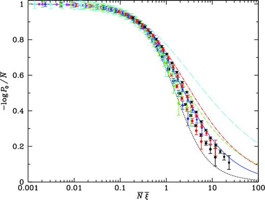
$Scaling statistic $\chi = - \ln P_0/{\bar{N}}$ plotted against scaling variable ${\bar{N}}{\bar{\xi }}$, for galaxies (squares) and haloes (circles). Lines show models, as in Fig. A1 in the Appendix. Colours red, blue, green, cyan, magenta show results for the full sample of haloes or substructure galaxies, and for random dilutions by successive factors of 2.$

Figure 1.

Scaling statistic |$\chi = - \ln P_0/{\bar{N}}$| plotted against scaling variable |${\bar{N}}{\bar{\xi }}$|⁠, for galaxies (squares) and haloes (circles). Lines show models, as in Fig. A1 in the Appendix. Colours red, blue, green, cyan, magenta show results for the full sample of haloes or substructure galaxies, and for random dilutions by successive factors of 2.

Open in new tab Download slide

Scaling curves for halo samples of different masses. Red symbols show all haloes, blue symbols show haloes with mass M > 5 × 1011 M⊙, and green symbols show M > 4 × 1012 M⊙. Circles, squares and triangles show the full catalogues and dilutions by successive factors of 2. Dotted (black) and solid (blue) lines show the minimal and negative binomial curves, as before, and the dashed (red) line shows the geometric hierarchical model of equation (A16).

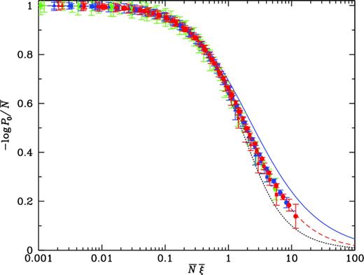
Figure 2.

Scaling curves for halo samples of different masses. Red symbols show all haloes, blue symbols show haloes with mass M > 5 × 10¹¹ M_⊙, and green symbols show M > 4 × 10¹² M_⊙. Circles, squares and triangles show the full catalogues and dilutions by successive factors of 2. Dotted (black) and solid (blue) lines show the minimal and negative binomial curves, as before, and the dashed (red) line shows the geometric hierarchical model of equation (A16).

Open in new tab Download slide

We see that the numerical results follow the predictions of hierarchical scaling, but this is not necessarily what is expected. Within the uncertainties of sampling a small number of objects, the amplitudes for haloes may be consistent with constant values, but those for mass, and especially for galaxies, are not. The normalization from |${\bar{\xi }}_k$| to |$S_k = {\bar{\xi }}_k/{\bar{\xi }}_2^{k-1}$| removes much of the variation with scale (the unnormalized five-point function for mass covers more than 10 decades), but the resulting S_k for galaxies are not constant, as shown in figs 5 and 6 of Fry et al. (2011), where the residual variation is still a factor of up to 10. Thus, we are faced with the fact that hierarchical void scaling is observed, but its premise does not hold. The halo model provides an explanation: in equations (19)–(22), |${\bar{\xi }}_2$| and the higher order |${\bar{\xi }}_k$| are all functions of |${\bar{N}}_h {\bar{\xi }}_h$|⁠, and |${\bar{N}}_h {\bar{\xi }}_h$| is linearly related to |${\bar{N}}_g {\bar{\xi }}_g$|⁠. Fig. 3 and equation 19 illustrate this in the simulation results. Fig. 3 shows |${\bar{N}}_g {\bar{\xi }}_g$| and |${\bar{N}}_h {\bar{\xi }}_h$| as a function of scale R, for the full samples and for the two-, four-, an eight-fold dilutions. Measured values are widely distributed; however, from equation (19), on large scales |${\bar{N}}_g {\bar{\xi }}_g$| is related to |${\bar{N}}_h {\bar{\xi }}_h$|⁠, as illustrated in Fig. 4. On large scales, where halo size is negligible, we expect to have no galaxies only if we have no haloes, a result also implied in the composition of generating functions. Fig. 5 shows P_{0, g} versus P_{0, h} for the same volumes.

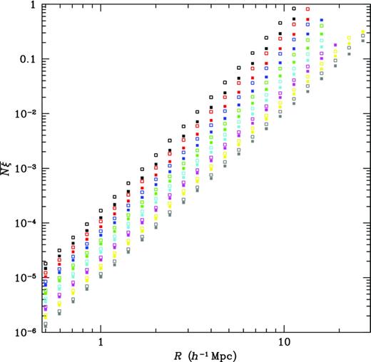
$${\bar{N}}_g {\bar{\xi }}_g$ and ${\bar{N}}_h {\bar{\xi }}_h$ plotted versus cell radius r. Symbols of the same colour show volumes of different radius for a fixed data sample. Colours black, red, blue, green, cyan, magenta, yellow show random dilutions by successive factors of two.$

Figure 3.

|${\bar{N}}_g {\bar{\xi }}_g$| and |${\bar{N}}_h {\bar{\xi }}_h$| plotted versus cell radius r. Symbols of the same colour show volumes of different radius for a fixed data sample. Colours black, red, blue, green, cyan, magenta, yellow show random dilutions by successive factors of two.

Open in new tab Download slide

$${\bar{N}}_g {\bar{\xi }}_g$ versus ${\bar{N}}_h {\bar{\xi }}_h$ for the same data plotted in Fig. 3. Symbols of the same colour show volumes of different radius for a fixed data sample: black shows the full sample; red, blue, green, cyan, magenta and yellow. show random dilutions by successive factors of 2. For coloured symbols (red) etc., both galaxies and haloes are diluted by same factor.$

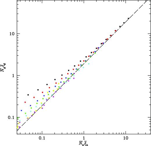
Figure 4.

|${\bar{N}}_g {\bar{\xi }}_g$| versus |${\bar{N}}_h {\bar{\xi }}_h$| for the same data plotted in Fig. 3. Symbols of the same colour show volumes of different radius for a fixed data sample: black shows the full sample; red, blue, green, cyan, magenta and yellow. show random dilutions by successive factors of 2. For coloured symbols (red) etc., both galaxies and haloes are diluted by same factor.

Open in new tab Download slide

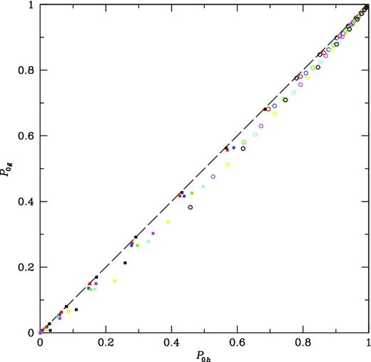
Figure 5.

Probability a volume is void of galaxies P_0g versus probability the same volume is void of haloes P_0h. Symbols of the same colour show volumes of different radius for a fixed data sample. Different colours show random dilutions by a factor of 2, black, red, blue, green, cyan, magenta, yellow.

Open in new tab Download slide

The halo model contains the requirement P_{0, g} = P_{0, h}, no galaxies means no haloes, no haloes means no galaxies, from equation (24) or from the fundamental sum over the occupancy of each halo, N_g = ∑N_i. From this, it is possible to obtain relations between void scaling curves for galaxies and their haloes, or between two different galaxy populations. Fig. 6 illustrates a mapping suggested by the halo model, from the halo curve to the galaxy curve. The figure shows the scaling statistic for galaxies |$-\ln P_{0,g} / {\bar{N}}_g$| (filled squares), for haloes |$-\ln P_{0,h} / {\bar{N}}_h$| (filled circles) and for haloes mapped vertically by the ratio of number

\begin{equation} {\chi _g \over \chi _h} = {-\log P_0 /{\bar{N}}_g \over -\log P_0/{\bar{N}}_h} = {{\bar{N}}_h \over {\bar{N}}_g} = {1 \over {\bar{N}}_i} = {1 \over 1.28}, \end{equation}

(29)

and horizontally by the ratio of the factors in |${\bar{N}}b^2$|⁠,

\begin{equation} {{\bar{N}}_g {\bar{\xi }}_g \over {\bar{N}}_h {\bar{\xi }}_h} = {\bar{N}}_i \, (b_g/b_h)^2 = (1.28) (1.22)^2 = 1.91 \end{equation}

(30)

(open circles). The mapping is indicated by arrows for a selected sample of points, but every open circle originates from a filled circle. The mapped halo curve and the galaxy curve are different for |${\bar{N}}{\bar{\xi }}\lesssim 1$|⁠, where resolved halo form factors affect the statistics (Fry et al. 2011), but they merge for |${\bar{N}}{\bar{\xi }}\gtrsim 1$|⁠. See also Tinker & Conroy (2009).

$Mappings between galaxy and halo scaling curves implied by the halo model. Filled squares show the void scaling curve for galaxies, $\chi _g = -\ln P_{0,g} / {\bar{N}}_g$ as a function of $x_g = {\bar{N}}_g {\bar{\xi }}_g$, and filled circles show the scaling curve for haloes, $\chi _h = -\ln P_{0,h} / {\bar{N}}_h$ as a function of $x_h = {\bar{N}}_h {\bar{\xi }}_h$. Open circles show the mapping of the halo data implied by the halo model, with χh scaled by the factor of ${\bar{N}}_h/{\bar{N}}_g = 1/1.28$, plotted as a function of xh scaled by the factor of 1.222 × 1.28 = 1.91. On large scales, this becomes the same as the galaxy curve. Straight lines show power-law behaviour x−ω with ω = 0.79, separated vertically by a factor of $(b_g/b_h)^{2\omega } \times ({\bar{N}}_g/{\bar{N}}_h)^{\omega -1} = 1.30$ or horizontally by a factor of $(b_g/b_h)^2 ({\bar{N}}_g/{\bar{N}}_h)^{1-1/\omega } = 1.39$.$

Figure 6.

Mappings between galaxy and halo scaling curves implied by the halo model. Filled squares show the void scaling curve for galaxies, |$\chi _g = -\ln P_{0,g} / {\bar{N}}_g$| as a function of |$x_g = {\bar{N}}_g {\bar{\xi }}_g$|⁠, and filled circles show the scaling curve for haloes, |$\chi _h = -\ln P_{0,h} / {\bar{N}}_h$| as a function of |$x_h = {\bar{N}}_h {\bar{\xi }}_h$|⁠. Open circles show the mapping of the halo data implied by the halo model, with χ_h scaled by the factor of |${\bar{N}}_h/{\bar{N}}_g = 1/1.28$|⁠, plotted as a function of x_h scaled by the factor of 1.22² × 1.28 = 1.91. On large scales, this becomes the same as the galaxy curve. Straight lines show power-law behaviour x^−ω with ω = 0.79, separated vertically by a factor of |$(b_g/b_h)^{2\omega } \times ({\bar{N}}_g/{\bar{N}}_h)^{\omega -1} = 1.30$| or horizontally by a factor of |$(b_g/b_h)^2 ({\bar{N}}_g/{\bar{N}}_h)^{1-1/\omega } = 1.39$|⁠.

Open in new tab Download slide

We obtain some inequalities comparing galaxies with their parent haloes. Write the scaling variable as |$x = {\bar{N}}{\bar{\xi }}$|⁠. All halo scaling curves lie above the minimal scaling curve, and so χ_h(x_h) > χ_min(x_h) > 1/x_h. With |$\chi _g/\chi _h = {\bar{N}}_g/{\bar{N}}_h$| and with |$x_g/x_h = b_g^2 {\bar{N}}_g/ b_h^2 {\bar{N}}_h$|⁠, this becomes a limit on χ_g,

\begin{equation} \chi _g = {{\bar{N}}_h \over {\bar{N}}_g} \, \chi _h = {({\bar{N}}_h b_h^2) \over ({\bar{N}}_g b_g^2)} \, {b_g^2 \over b_h^2} \, \chi _h = {x_h \over x_g} \, \chi _h {b_g^2 \over b_h^2} \, > {b_g^2 \over b_h^2} \, {1 \over x_g}. \end{equation}

(31)

Since b(m) is an increasing function of mass and b_g (equation 17) is weighted to larger m than b_h (equation 16), we thus expect χ_g > 1/x_g. As a horizontal scaling, we expect χ_g = χ_h at a value

\begin{equation} {x_g \over x_h} > {b_g^2 {\bar{N}}_g \over b_h^2 {\bar{N}}_h}. \end{equation}

(32)

Since both b_g/b_h > 1 and |${\bar{N}}_g/{\bar{N}}_h > 1$|⁠, we expect that in general, galaxy scaling curve will be to the right of the halo scaling curve.

To the extent that the scaling curve can be represented as a power law, χ = Ax^−ω (Balian & Schaeffer 1988), we can write quantitative relations. Power-law behaviour implies a vertical mapping between two scaling curves at the same value of x,

\begin{equation} {\chi _g \over \chi _h} = \Bigl ( {b^2_g \over b^2_h} \Bigr )^\omega \Bigl ( {{\bar{n}}_g \over {\bar{n}}_h} \Bigr )^{\omega -1}, \end{equation}

(33)

or a horizontal mapping,

\begin{equation} {x_g \over x_h} = {b^2_g \over b^2_h} \, \Bigl ( {{\bar{n}}_g \over {\bar{n}}_h} \Bigr )^{1-1/\omega } \end{equation}

(34)

between two curves at the same value of χ. Since ω is often near 1, the horizontal mapping is typically much more dependent on relative bias and only weakly on relative number. This horizontal mapping is illustrated in Fig. 6, with ω = 0.79.

We can compare two galaxy populations, say i and j. The simpler case is when both derive from essentially the same halo population; then we have the mappings

\begin{eqnarray} {\chi _i \over \chi _j} &=& {{\bar{n}}_j \over {\bar{n}}_i}, \end{eqnarray}

(35)

\begin{eqnarray} {x_i \over x_j} &=& {b_i^2 \over b_j^2} \, { {\bar{n}}_i \over {\bar{n}}_j}. \end{eqnarray}

(36)

With a power-law halo scaling function χ_h = Ax^−ω, we find the horizontal mapping χ_i = χ_j at

\begin{equation} {x_i \over x_j} = {b_i^2 \over b_j^2} \, \left( {{\bar{n}}_i \over {\bar{n}}_j} \right)^{1-1/\omega }. \end{equation}

(37)

If halo scaling follows the minimal model, with ω ≈ 1, number density does not enter at all. For the negative binomial model, on scales of interest ω ≈ 0.8 and 1 − 1/ω ≈ −0.25, still a very weak dependence. Such a weak dependence on number means that we can expect scaling curves for populations with higher bias to be shifted to the right, by a factor of approximately |$b_{\rm rel}^2$|⁠, or shifted upwards, by a slightly larger factor.

We can also compare galaxy populations that derive from distinct halo populations that have different number density and correlation strength, as long as they follow the same scaling curves, as in Fig. 2. Here, it is the relative bias b_{g, i}/b_{h, i} and relative number density |${\bar{n}}_{g,i} / {\bar{n}}_{h,i}$|⁠, etc., that appear in the scaling relation. For power law χ ∼ x^−ω, this reduces to the single horizontal scaling

\begin{equation} {x_i \over x_j} = {(b_g/b_h)_i^2 \over (b_g/b_h)_j^2} \, \left[ {({\bar{n}}_g/{\bar{n}}_h)_i \over ({\bar{n}}_g/{\bar{n}}_h)_j} \right]^{1-1/\omega }. \end{equation}

(38)

Finally, we present results for voids in the mass or dark matter distribution. The number of dark matter particles is so large that unless diluted substantially, only very small volumes are empty. We begin with a random sample of one out of eight, or 256³ particles, for which we compute the full P_N for volumes with R = 0.2 h⁻¹ Mpc to R = 25 h⁻¹ Mpc by factors of |$\sqrt{2}$|⁠. We then take advantage of the generating function to plot results for dilutions by a factor of λ,

\begin{equation} P_0(\lambda ) = G(1-\lambda ), \end{equation}

(39)

for λ = 2^k/2, k = 0 to 20, or effective number of points from 256³ = 16 777 216 down to 16 284. Fig. 7 shows the scaling function |$\chi = -\ln P_0 / {\bar{N}}$| plotted against the scaling variable |${\bar{N}}{\bar{\xi }}$| for the full sample and the 20 dilutions. We note that Croton et al. (2004a) do not test scaling, but present results for only one density, which from their simulation parameters should be equivalent to the second curve below the median in Fig. 7.

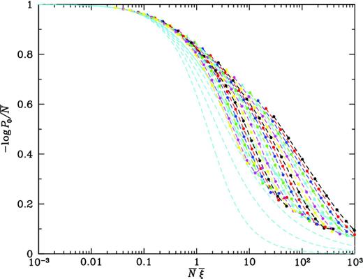
$Scaling function $\chi = - \ln P_0/{\bar{N}}$ plotted against scaling variable ${\bar{N}}{\bar{\xi }}$ for subsets of dark matter particles. The top (black) curve is derived from a subsample of 2563 = 16 777 312 points, and each curve below that is diluted by a further factor of $\sqrt{2}$; the final curve, diluted by a factor of 1024, then represents 16 384 points. Dashed (cyan) curves show the behaviour expected from gravitational instability (equation A6), smoothed for spectral index n = +1, 0, −1, −2 and −3 (bottom to top).$

Figure 7.

Scaling function |$\chi = - \ln P_0/{\bar{N}}$| plotted against scaling variable |${\bar{N}}{\bar{\xi }}$| for subsets of dark matter particles. The top (black) curve is derived from a subsample of 256³ = 16 777 312 points, and each curve below that is diluted by a further factor of |$\sqrt{2}$|⁠; the final curve, diluted by a factor of 1024, then represents 16 384 points. Dashed (cyan) curves show the behaviour expected from gravitational instability (equation A6), smoothed for spectral index n = +1, 0, −1, −2 and −3 (bottom to top).

Open in new tab Download slide

The dark matter results do not follow the scaling implied by gravitational instability, but this is because most of the volumes sampled are not in the large-scale, perturbative regime. To compare with perturbative gravitational instability, Fig. 8 shows results restricted to large volumes, R = 6.3, 8.8, 12.5 and R > 17 h⁻¹ Mpc. For sufficiently large R, the measurements seem to approach the curve predicted for gravitational instability for the appropriate value of n ≈ −2, where |${\rm d}(\ln {\bar{\xi }}) / {\rm d}(\ln R) = - (3+n)$|⁠.

The small R behaviour of the halo model also has its own, modified scaling behaviour, with power-law correlations |${\bar{\xi }}_k \propto R^{-(k-1) \gamma + \delta }$|⁠, where γ = (9 + 3n)/(5 + n) and δ = (3 + n)p^′/(5 + n); p^′ characterizes the small mass behaviour of the halo mass function, |${\rm d}n/{\rm d}m \sim \nu ^{p^{\prime }}/m^2$| (Ma & Fry 2000a; Scoccimarro et al. 2001). In terms of |${\bar{\xi }}_2$|⁠, this is

\begin{equation} {\bar{\xi }}_k \sim {\bar{\xi }}^{(k-1) (1+\Delta ) - \Delta }, \end{equation}

(40)

with Δ = δ/γ = p^′/(3 − p^′), independent of spectral index n. This dependence implies a modified scaling,

\begin{equation} -\ln P_0/{\bar{N}}= 1 + {\bar{\xi }}^{-\Delta } \; \psi ( {\bar{N}}{\bar{\xi }}^{1+\Delta }), \end{equation}

(41)

expected to hold at small R. This behaviour was anticipated numerically by Colombi, Bouchet & Hernquist (1996), who also point out that this modified scaling cannot persist on all scales. Fig. 9 shows the success of this scaling for p^′ = −0.2, Δ = −0.0625. This value is different, even in sign, from the scaling exponent inferred from low-order hierarchical amplitudes, although both are numerically small, and may indicate a change in the mass dependence of halo mass function at smaller masses. In evaluating results for dark matter particles, we must also keep in mind that it is possible that some effect remains of the initial grid. Colombi et al. (1995) suggest that void results should be reliable only P₀ ≳ 1/e, but we see no change of behaviour on different sides of this boundary.

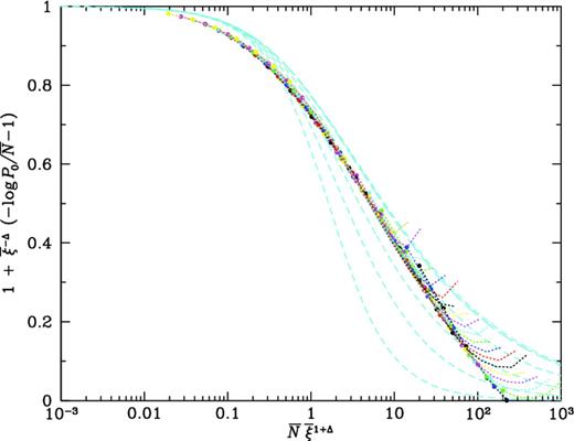
The curves of Fig. 7 scaled as in equation (41), with Δ = −0.0625. Points are plotted for R < 1 h−1 Mpc, while connecting lines are extended for all R. Dashed (cyan) curves are as in Fig. 7; measured values typically lie between −2 and −1.

Figure 9.

The curves of Fig. 7 scaled as in equation (41), with Δ = −0.0625. Points are plotted for R < 1 h⁻¹ Mpc, while connecting lines are extended for all R. Dashed (cyan) curves are as in Fig. 7; measured values typically lie between −2 and −1.

Open in new tab Download slide

$Scaling curves $\chi = - \ln P_0/{\bar{N}}$ versus ${\bar{N}}{\bar{\xi }}$ for point distributions that track dark matter, for large volumes: R = 6.3 (green), R = 8.8 (blue), R = 12.5 (red) and R > 16 h−1 Mpc (black). Filled symbols show measured results; open symbols show gravitational instability results smoothed for effective spectral index n, where $3+n = - {\rm d}\,\ln {\bar{\xi }}/ {\rm d}\,\ln R$. For these scales, n takes on values −2 < n < −1. Dashed (cyan) curves are as in Fig. 7.$

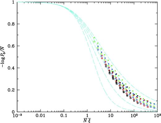
Figure 8.

Scaling curves |$\chi = - \ln P_0/{\bar{N}}$| versus |${\bar{N}}{\bar{\xi }}$| for point distributions that track dark matter, for large volumes: R = 6.3 (green), R = 8.8 (blue), R = 12.5 (red) and R > 16 h⁻¹ Mpc (black). Filled symbols show measured results; open symbols show gravitational instability results smoothed for effective spectral index n, where |$3+n = - {\rm d}\,\ln {\bar{\xi }}/ {\rm d}\,\ln R$|⁠. For these scales, n takes on values −2 < n < −1. Dashed (cyan) curves are as in Fig. 7.

Open in new tab Download slide

DISCUSSION

The implication of the halo model for void probability on large scales is simple: to have no galaxies means no haloes, no haloes means no galaxies. This point cluster limit of the halo model provides a natural answer to the otherwise puzzling question, Why do voids obey the hierarchical scaling when the correlation functions do not satisfy the hierarchical premise, constant S_n. In the limit that the volume considered is large compared to halo sizes, void of galaxies means void of haloes, the void probability P₀ is the same, and scaling curves are related by number and by clustering strength or bias. Since |${\bar{N}}_g\,>\,{\bar{N}}_h$| (a halo contains one or more galaxies) and |${\bar{\xi }}_g\, >\, {\bar{\xi }}_h$| (bias is an increasing function of mass), we anticipate points on the scaling plot move down and to the left.

In the simulations as well as in observations, the negative binomial scaling curve is a good approximation to that for galaxies; the weak clustering lognormal curve is much less favoured, and the more strongly clustered lognormal even less so. We expect the void scaling relation to provide different scaling curves for different galaxy populations; that galaxy results are often in agreement with the negative binomial curve can be attributed to the number density and clustering strength of typical galaxies. With different results for different galaxy populations, in a direction consistent with relative bias and number density, we conclude that there is no fundamental reason that galaxies follow the negative binomial scaling curve, but that this follows from typical galaxy parameters.

The success of void scaling for galaxies requires that the underlying halo distribution follows the hierarchical pattern of higher order clustering. In our simulations (Fry et al. 2011), the halo S_k,h are approximately constant, roughly S_3,h ≈ 1, S_4,h ≈ 2 and S_5,h ≈ 3, over a limited range of scales squeezed between the finite size of the simulation on the large end and the ability to separate extended objects on the small end. These values of the S_k,h do not change much for different mass ranges. More important, as seen in Fig. 2, different halo samples have remarkably similar scaling curves: for mass thresholds ranging over a factor of 20 and number densities different by a factor of more than 4, the scaling curves are indistinguishable and seem to follow well the geometric halo mode curve of equation (A16). The scaling is important, because there is essentially no direct observational information for S_k,h. What results do exist are only for much higher mass thresholds: Jing (1990) measures the void scaling function for ACO clusters and Cappi, Maurogordato & Lachieze-Rey (1991) for samples defined by Postman, Geller & Huchra (1986) and Tully (1987), but their results only reach |${\bar{N}}{\bar{\xi }}\lesssim 2$|⁠, for which all model scaling curves are much the same. Jing & Zhang (1989) find that Abell clusters have a hierarchical three-point function with amplitude independent of richness class, and Cappi & Maurogordato (1995) also find, to a degree, constant S_k amplitudes for Abell and ACO clusters (but with a systematic difference between northern and southern galactic hemispheres), with numerical values S₃ ≈ 3, S₄ ≈ 15, S₅ ≈ 100, appropriate to the high threshold, rare halo limit S_k = k^{k − 2} of Bernardeau & Schaeffer (1999). These do not apply directly to statistics of haloes that host galaxies, including single galaxies and so extend down to galaxy masses; a theory that predicts the halo amplitudes S_k,h or the halo scaling curve for mass thresholds of 10¹¹ or 10¹² M_⊙ has yet to be found.

Dark matter behaves differently. For dark matter, the behaviour of voids depends strongly on the density of particles. In the quasi-linear regime on large scales, the behaviour seems to follow the predictions of gravitational instability. For mass, there is no smallest object, no smallest cluster, and for any scale there are always clusters smaller and larger than that size. The halo model has implications for high-order functions, Small scales follow a modified scaling predicted by the halo model, as in equation (41).

Halo model mappings have been derived in order to apply to observational data. Tinker et al. (2008) present in their Fig. 7(d) void scaling curves for SDSS blue and red galaxies in which the locus for red galaxies is shifted substantially to larger values of |${\bar{N}}{\bar{\xi }}$|⁠; similar results are found for red and blue 2dFGRS galaxies by Croton et al. (2007). Fig. 10 shows the SDSS data (filled circles) and the results of halo model scalings applied to red and blue galaxies for three different assumptions about the underlying haloes: assuming red and blue galaxies reside in the same haloes (open triangles), assuming a power-law halo scaling curve with ω = 1 (open circles), and assuming their parent haloes trace same halo scaling curve (open squares), using the values b_red = 1.02, b_blue = 0.85, n_red = 0.00328, |$n_{\rm blue}= 0.00433 \, h^3 \, {\rm Mpc}^{-3}$| and ratios (b_g/b_h)_red = 1.53, (n_g/n_h)_red = 1.93, (b_g/b_h)_blue = 1.18, (n_g/n_h)_blue = 1.21, computed from analytic halo occupation distributions for red and blue samples given by Tinker et al. (2008). Blue squares and red triangles begin to show departures from simple scalings, which should apply only in the large-scale limit. The last, relative scaling is perhaps the most realistic, but the halo assumptions overlap and all of the scalings behave similarly. This is a confirmation that the ideas of the halo model apply to observations, as well as to simulations.

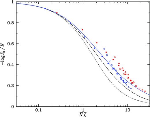
Figure 10.

Void scaling for SDSS red and blue galaxies. Solid circles show SDSS data from Tinker et al. (2008). Open triangles show direct mapping, appropriate if the two samples inhabit the same haloes. Open squares show mapping assuming the two samples derive not from the same haloes but from haloes that follow the same scaling curve. Open circles are mapped only by bias, as appropriate for a power-law scaling with ω = 1.

Open in new tab Download slide

The void scaling results illustrate yet another success of the halo model in describing non-linear phenomena that it was not designed and not optimized to explain. Applied to dark matter, the model may still be only an approximation, but for galaxies, on scales where details of the structure of haloes are irrelevant, it is almost necessarily true: the total number of galaxies is the sum over haloes of the number of galaxies in each halo, and the combinatoric results of the halo model are independent of whether there is such a thing as a universal profile shape or not.

The question of why is it that voids in the galaxy distribution obey hierarchical scaling when their correlations do not follow the hierarchical pattern was raised by Darren Croton at the Summer 2007 workshop on Modelling Galaxy Clustering at the Aspen Center for Physics. We thank David Weinberg for providing the SDSS results. JNF acknowledges support from the City of Paris, Research in Paris programme and thanks the Pauli Institute for Theoretical Physics, University of Zürich, and the Institut d’Astrophysique de Paris for hospitality during this work. This research has made use of NASA's Astrophysics Data System.

REFERENCES

Alimi

J.-M.

Blanchard

A.

Schaeffer

R.

,

ApJ

,

1990

, vol.

349

pg.

L5

Crossref

Search ADS

Balian

R.

Schaeffer

R.

,

ApJ

,

1988

, vol.

335

pg.

L43

Crossref

Search ADS

Bernardeau

F.

,

ApJ

,

1992

, vol.

392

pg.

1

Crossref

Search ADS

Bernardeau

F.

,

A&A

,

1994

, vol.

291

pg.

697

Bernardeau

F.

Schaeffer

R.

,

A&A

,

1999

, vol.

349

pg.

697

Bouchet

F. R.

Strauss

M. A.

Davis

M

Fisher

K. B.

Yahil

A.

Huchra

J. P.

,

ApJ

,

1993

, vol.

417

pg.

36

Crossref

Search ADS

Cappi

A.

Maurogordato

S.

,

ApJ

,

1995

, vol.

438

pg.

507

Crossref

Search ADS

Cappi

A.

Maurogordato

S.

Lachieze-Rey

M.

,

A&A

,

1991

, vol.

243

pg.

28

Carruthers

P.

,

ApJ

,

1991

, vol.

380

pg.

24

Crossref

Search ADS

Carruthers

P.

Minh

D.-V.

,

Phys. Lett.

,

1983

, vol.

131B

pg.

116

Crossref

Search ADS

Carruthers

P.

Shih

C. C.

,

Phys. Lett.

,

1983

, vol.

127B

pg.

242

Crossref

Search ADS

Carruthers

P.

Shih

C. C.

,

Int. J. Mod. Phys. A

,

1987

, vol.

2

pg.

1447

Crossref

Search ADS

Coles

P.

Jones

B.

,

MNRAS

,

1991

, vol.

248

pg.

1

Crossref

Search ADS

Colombi

S.

Bouchet

F. R.

Schaeffer

R.

,

ApJS

,

1995

, vol.

96

pg.

401

Crossref

Search ADS

Colombi

S.

Bouchet

F. R.

Hernquist

L.

,

ApJ

,

1996

, vol.

465

pg.

14

Crossref

Search ADS

Colombi

S.

Chodorowski

M. J.

Teyssier

R.

,

MNRAS

,

2007

, vol.

375

pg.

348

Crossref

Search ADS

Conroy

C.

et al. ,

ApJ

,

2005

, vol.

635

pg.

990

Crossref

Search ADS

Croton

D. J.

et al. ,

MNRAS

,

2004a

, vol.

352

pg.

828

Crossref

Search ADS

Croton

D. J.

et al. ,

MNRAS

,

2004b

, vol.

352

pg.

1232

Crossref

Search ADS

Croton

D. J.

Norberg

P.

Gaztañaga

E.

Baugh

C. M.

,

MNRAS

,

2007

, vol.

379

pg.

1562

Crossref

Search ADS

Elizalde

E.

Gaztañaga

E.

,

MNRAS

,

1992

, vol.

254

pg.

247

Crossref

Search ADS

Fall

S. M.

Geller

M.

Jones

B. J. T.

White

S. D. M.

,

ApJ

,

1976

, vol.

205

pg.

L121

Crossref

Search ADS

Fry

J. N.

,

ApJ

,

1984

, vol.

279

pg.

499

Crossref

Search ADS

Fry

J. N.

,

ApJ

,

1986

, vol.

306

pg.

358

Crossref

Search ADS

Fry

J. N.

Giovanelli

R.

Haynes

M. P.

Melott

A. L.

Scherrer

R. J.

,

ApJ

,

1989

, vol.

340

pg.

11

Crossref

Search ADS

Fry

J. N.

Colombi

S.

Fosalba

P.

Balaraman

A.

Szapudi

I. Teyssier R.

,

MNRAS

,

2011

, vol.

415

pg.

153

Crossref

Search ADS

Gaztañaga

E

,

ApJ

,

1992

, vol.

398

pg.

L17

Crossref

Search ADS

Gaztañaga

E.

,

MNRAS

,

1994

, vol.

268

pg.

913

Crossref

Search ADS

Gaztañaga

E.

Yokohama

J.

,

ApJ

,

1993

, vol.

403

pg.

450

Crossref

Search ADS

Ghosh

D.

Deb

A.

Ghosh

J.

Chattopadhyay

R.

Kayum

Jafri A.

Azizar

Rahman M.

Sarkar

S. R.

,

Astropart. Phys.

,

2001

, vol.

15

pg.

329

Crossref

Search ADS

Greenwood

M.

Yale

G. U.

,

J. R. Stat. Soc. A

,

1920

, vol.

83

pg.

255

Crossref

Search ADS

Hamilton

A. J. S.

,

ApJ

,

1985

, vol.

292

pg.

L35

Crossref

Search ADS

Hamilton

A. J. S.

,

ApJ

,

1988

, vol.

332

pg.

67

Crossref

Search ADS

Hegyi

S.

,

Phys. Lett. B

,

1992

, vol.

274

pg.

214

Crossref

Search ADS

Hubble

E.

,

ApJ

,

1934

, vol.

79

pg.

8

Crossref

Search ADS

Jing

Y.-P.

,

A&A

,

1990

, vol.

233

pg.

309

Jing

Y.-P.

Zhang

J.-L.

,

ApJ

,

1989

, vol.

342

pg.

639

Crossref

Search ADS

Klauder

J. R.

Sudarshan

E. C. G.

,

Fundamentals of Quantum Optics

,

1968

New York

Benjamin

Google Scholar

Google Preview

OpenURL Placeholder Text

WorldCat

Ma

C.-P.

Fry

J. N.

,

ApJ

,

2000a

, vol.

538

pg.

L107

Crossref

Search ADS

Ma

C.-P.

Fry

J. N.

,

ApJ

,

2000b

, vol.

543

pg.

503

Crossref

Search ADS

Malik

S.

,

Phys. Rev. D

,

1996

, vol.

54

pg.

3655

Crossref

Search ADS

Maurogordato

S.

Lachièze-Rey

M.

,

ApJ

,

1987

, vol.

320

pg.

13

Crossref

Search ADS

Maurogordato

S.

Schaeffer

R.

da Costa

L. N.

,

ApJ

,

1992

, vol.

390

pg.

17

Crossref

Search ADS

Mekjian

A. Z.

,

ApJ

,

2007

, vol.

655

pg.

1

Crossref

Search ADS

Mo

H. J.

Jing

Y. P.

White

S. D. M.

,

MNRAS

,

1997

, vol.

284

pg.

189

Crossref

Search ADS

Neyman

J.

Scott

E. L.

Shane

C. D.

,

ApJ

,

1953

, vol.

117

pg.

92

Crossref

Search ADS

Peebles

P. J. E.

,

The Large-Scale Structure of the Universe

,

1980

Princeton, NJ

Princeton Univ. Press

Google Scholar

Google Preview

OpenURL Placeholder Text

WorldCat

Politzer

H. D.

Wise

M. B.

,

ApJ

,

1984

, vol.

285

pg.

L1

Crossref

Search ADS

Postman

M.

Geller

M. J.

Huchra

J. P.

,

AJ

,

1986

, vol.

91

pg.

1267

Crossref

Search ADS

Ross

A. J.

Brunner

R. J.

Myers

A. D.

,

ApJ

,

2006

, vol.

649

pg.

48

Crossref

Search ADS

Ross

A. J.

Brunner

R. J.

Myers

A. D.

,

ApJ

,

2007

, vol.

665

pg.

67

Crossref

Search ADS

Saslaw

W. C.

Hamilton

A. J. H.

,

ApJ

,

1984

, vol.

276

pg.

13

Crossref

Search ADS

Schaeffer

R.

,

A&A

,

1984

, vol.

134

pg.

L15

Scoccimarro

R.

Sheth

R. K.

Hui

L.

Jain

B.

,

ApJ

,

2001

, vol.

546

pg.

20

Crossref

Search ADS

Sheth

R. K.

,

MNRAS

,

1995

, vol.

274

pg.

213

Crossref

Search ADS

Sheth

R. K.

,

MNRAS

,

1996

, vol.

281

pg.

1124

Crossref

Search ADS

Sheth

R. K.

Saslaw

W. C.

,

ApJ

,

1994

, vol.

437

pg.

35

Crossref

Search ADS

Szalay

A. S.

,

ApJ

,

1988

, vol.

333

pg.

21

Crossref

Search ADS

Szapudi

I.

Szalay

A. S.

,

ApJ

,

1993

, vol.

414

pg.

493

Crossref

Search ADS

Teich

M. C.

Campos

R. A.

Saleh

B. E. A.

,

Phys. Rev. D

,

1987

, vol.

36

pg.

2649

Crossref

Search ADS

Teyssier

R.

,

A&A

,

2002

, vol.

385

pg.

337

Crossref

Search ADS

Tinker

J. L.

Conroy

C.

,

ApJ

,

2009

, vol.

691

pg.

633

Crossref

Search ADS

Tinker

J. L.

Conroy

C.

Norberg

P.

Patiri

S. G.

Weinberg

D. H.

Warren

M. S.

,

ApJ

,

2008

, vol.

686

pg.

53

Crossref

Search ADS

Tully

R. B.

,

ApJ

,

1987

, vol.

323

pg.

1

Crossref

Search ADS

Vogeley

M. S.

Geller

M. J.

Park

C.

Huchra

J. P.

,

AJ

,

1994

, vol.

108

pg.

745

Crossref

Search ADS

White

S. D. M.

,

MNRAS

,

1979

, vol.

186

pg.

145

Crossref

Search ADS

Yang

W.

Xuan

R.

Li

L.

,

Geochem.

,

1983

, vol.

1

pg.

52

APPENDIX A: MODELS

In this Appendix, we present several models with specific analytic forms for the void scaling function |$\chi ({\bar{N}}{\bar{\xi }})$|⁠, useful against which to compare observational and numerical results. Many of these models, introduced previously in a variety of different contexts (see Fry 1986; Mekjian 2007), can be realized as halo models with a Poisson halo distribution; several were discussed by Sheth (1996). With mean μ, probabilities p_n = μⁿ e^{− μ}/n!, the Poisson generating function is

\begin{equation} g(z) = \sum _{n=0}^\infty {1 \over n!} \, \mu ^n \, {\rm e}^{-\mu } \, z^n = {\rm e}^{\mu (z-1)} ; \end{equation}

(A1)

in particular, the void probability is |$P_0 = {\rm e}^{-{\bar{N}}_h} = {\rm e}^{-{\bar{N}}/{\bar{N}}_i}$|⁠. For an unclustered halo distribution, correlations of galaxy number are given by the last term in equations (10)–(13), and a Poisson halo distribution is always hierarchical of a sort, with scaling function |$\chi = - \ln P_0/ {\bar{N}}= 1/{\bar{N}}_i$|⁠, scaling variable |${\bar{N}}{\bar{\xi }}= {\bar{N}}_i \, {\bar{\mu }}_{2,i}$| and amplitudes |$S_k = {\bar{\mu }}_{k,i} / {\bar{\mu }}_{2,i}^{k-1}$| all determined by the occupation distribution (although not every occupation distribution has constant S_k). Fig. A1 compares models detailed in the following.

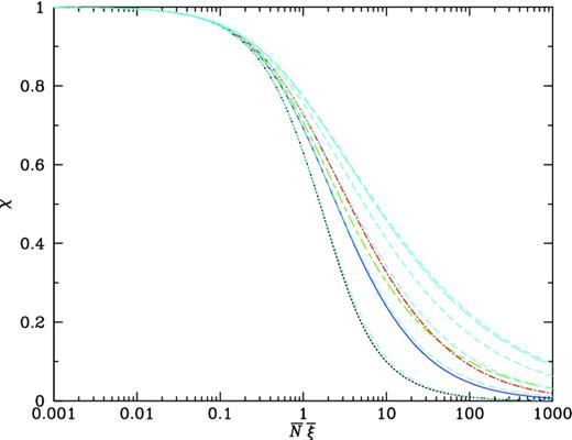
$Model void scaling functions $\chi ({\bar{N}}{\bar{\xi }})$. The solid (blue) line shows the negative binomial model (equation A14); the doted (black) line shows the minimal model (equation A5); the short dashed/long dashed (green) line shows the quasi-equilibrium model (equation A20); the dot–dashed (red) line shows the Schaeffer or lognormal model (equation A21); the long dashed (cyan) curve shows the gravitational instability prediction (Section A6); and the short dashed (cyan) curves show the smoothed gravitational instability result for effective power index n = −3, −2, −1, 0 and +1 (top to bottom).$

Figure A1.

Model void scaling functions |$\chi ({\bar{N}}{\bar{\xi }})$|⁠. The solid (blue) line shows the negative binomial model (equation A14); the doted (black) line shows the minimal model (equation A5); the short dashed/long dashed (green) line shows the quasi-equilibrium model (equation A20); the dot–dashed (red) line shows the Schaeffer or lognormal model (equation A21); the long dashed (cyan) curve shows the gravitational instability prediction (Section A6); and the short dashed (cyan) curves show the smoothed gravitational instability result for effective power index n = −3, −2, −1, 0 and +1 (top to bottom).

Open in new tab Download slide

Minimal Poisson model

A Poisson sum of clusters with mean μ with Poisson occupancy distribution with mean ν has

\begin{equation} G = g_h[g_i(z)] = \exp \left( \mu \, [ {\rm e}^{\nu (z-1)} - 1 ] \right). \end{equation}

(A2)

From derivatives of G we have moments |$\mathop {{\langle }}\nolimits N^{[k]} \mathop {{\rangle }}\nolimits$| (equation 4),

\begin{equation} {\bar{N}} = G^{\prime }(1) = \mu \nu , \end{equation}

(A3)

\begin{eqnarray} {\bar{N}}^2 {\bar{\xi }} = G^{\prime \prime }(1) - [G^{\prime }(1)]^2 = \mu \nu ^2, \end{eqnarray}

(A4)

from which we obtain |$\nu = {\bar{N}}{\bar{\xi }}$|⁠, |$\mu = 1/{\bar{\xi }}$|⁠, void probability |$P_0 = G(0) = \exp \left[ - (1 - {\rm e}^{-{\bar{N}}{\bar{\xi }}})/{\bar{\xi }}\right]$| and thus

\begin{equation} \chi = {1 - {\rm e}^{-{\bar{N}}{\bar{\xi }}} \over {\bar{N}}{\bar{\xi }}}. \end{equation}

(A5)

This minimal hierarchical model, with S_k = 1 for all k, saturates the Schwarz inequality requirement that the hierarchical amplitudes obey |$S_{2m} \, S_{2n} \ge S_{m+n}^{\, 2}$| (Fry 1986).

A Poisson occupation distribution formally includes possibility empty haloes. The same result can be achieved by excising empty haloes and rescaling (Fry et al. 2011), so that the occupation generating function becomes

\begin{equation} g_i(z) = {{\rm e}^{\nu (z-1)} - {\rm e}^{-\nu } \over 1 - {\rm e}^{-\nu }}. \end{equation}

(A6)

The remainder of the calculation is straightforward; although the relation between ν and |${\bar{N}}_i$| changes, again |$\nu = {\bar{N}}{\bar{\xi }}$| and |$\chi = (1 - {\rm e}^{-{\bar{N}}{\bar{\xi }}})/{\bar{N}}{\bar{\xi }}$|⁠.

Equation (A5) is the limit a → ∞ of the hypergeometric model of Mekjian (2007), which has

\begin{equation} \chi _a = {(1 + {\bar{N}}{\bar{\xi }}/a)^{1-a} - 1 \over (1-a) {\bar{N}}{\bar{\xi }}/ a}. \end{equation}

(A7)

The minimal model scaling curve is plotted as the dotted (black) line in Fig. A1.

Negative binomial model

The negative binomial distribution with mean |${\bar{N}}$| and parameter K (also called Pascal, if K is an integer, or Pólya distribution if K is real), has count probabilities

\begin{equation} P_N = { (N+K-1)! \over N! \, (K-1)!} {({\bar{N}}/K)^N \over (1 + {\bar{N}}/K)^{N+K} }. \end{equation}

(A8)

For K = 1, this reduces to the Bose–Einstein distribution, and is sometimes also referred to as modified Bose–Einstein. This distribution appears in the frequency of industrial accidents (Greenwood & Yale 1920), the distribution of ancient meteorites found in China (Yang, Xuan & Li 1983), in quantum optics (Klauder &. Sudarshan 1968), and in the multiplicity of charged particles produced in high-energy collisions (Carruthers & Shih 1983, 1987; Carruthers 1991) and cosmic ray showers (Teich, Campos & Saleh 1987), as well as in large-scale structure (Neyman, Scott & Shane 1953; Carruthers & Minh 1983; Carruthers & Shih 1983; Carruthers 1991; Elizalde & Gaztañaga 1992; Gaztañaga 1992; Gaztañaga & Yokohama 1993), where it is often found to be a good approximation to the observed scaling curve of galaxies.

The negative binomial can be realized as a Poisson sum of clusters with logarithmic occupation distribution (Sheth 1995). The halo and occupation generating functions are

\begin{eqnarray} g_i(z) &=& \sum _{n=1}^\infty {-1 \over \ln (1-p)} \, {p^n \over n} \, z^n = {\ln (1-pz) \over \ln (1-\,p\,)}, \end{eqnarray}

(A9)

\begin{eqnarray} G(z) &=& \exp \left( \mu \, \Bigl [ {\ln (1-pz) \over \ln (1-\,p\,)} - 1 \Bigr ] \right). \end{eqnarray}

(A10)

The probability of a void is G(0) = e^{− μ} and |$\chi = \mu /{\bar{N}}$|⁠; it is only necessary to relate these to moments |${\bar{N}}$|⁠, |${\bar{\xi }}$| obtained from G^′(0) and G^′^′(0) as in equations (A3), (A4),

\begin{eqnarray} {\bar{N}}= -{\mu p /(1-p) \over \ln (1-p)}, \qquad {\bar{N}}^2 {\bar{\xi }}= -{\mu p^2 / (1-p)^2 \over \ln (1-p)}. \end{eqnarray}

(A11)

Then,

\begin{equation} \chi = {\mu \over {\bar{N}}} = {1-p \over p} \, \ln (1-p), \end{equation}

(A12)

\begin{equation} {\bar{N}}{\bar{\xi }}= {p \over 1-p}, \end{equation}

(A13)

\begin{equation} \chi = {\mu \over {\bar{N}}} = {1-p \over p} \, \ln (1-p) = { \ln (1 + {\bar{N}}{\bar{\xi }}) \over {\bar{N}}{\bar{\xi }}}. \end{equation}

(A14)

It has been suggested that convergence of the logarithmic series defined by equation (8) with S_k = (k − 1)! limits |${\bar{N}}{\bar{\xi }}< 1$|⁠; but the probability generating function formulation has no restriction.

Equation (A14) is the limit a → 1 of the hypergeometric model of Mekjian (2007). The negative binomial model scaling curve is plotted as the solid (blue) line in Fig. A1.

Geometric hierarchical model

An occupancy distribution with probability p_n ∝ pⁿ for n ≥ 1 has occupancy generating function g_i(z) = z(1 − p)/(1 − pz) and

\begin{eqnarray} G(z) &=& \exp \left( \mu \, \Bigl [ {z(1-p) \over 1-pz} - 1 \Bigr ] \right). \end{eqnarray}

(A15)

From the first and second moments, |${\bar{N}}= \mu p/(1-p)$| and |${\bar{N}}^2 {\bar{\xi }}= 2 \mu p/(1-p)^2$|⁠, we find |$p = {\frac{1}{2}}{\bar{N}}{\bar{\xi }}/ (1 + {\frac{1}{2}}{\bar{N}}{\bar{\xi }})$| and

\begin{equation} \chi = {\mu \over {\bar{N}}} = 1-p = {1 \over 1 + {\textstyle {1 \over 2}}{\bar{N}}{\bar{\xi }}}. \end{equation}

(A16)

The geometric halo model is the case a = 2 of the hypergeometric model of Mekjian (2007), the model of Hamilton (1988) with |$Q = {\frac{1}{2}}$|⁠, and also the ω = 1 instance of the form |$\chi = 1/(1 + {\bar{N}}{\bar{\xi }}/2\omega )^\omega$| cited in Alimi, Blanchard & Schaeffer (1990). Although not plotted, the geometric model falls between the minimal and negative binomial curves in Fig. A1.

Quasi-equilibrium model

Saslaw & Hamilton (1984) apply thermodynamics to obtain a gravitational quasi-equilibrium distribution function. The resulting distribution is once again a halo model, a Poisson sum of haloes, with Borel occupation distribution (Sheth & Saslaw 1994; Sheth 1996),

\begin{equation} p_n = {1 \over n!} \, (nb)^{n-1} \, {\rm e}^{-nb}, \end{equation}

(A17)

and with total count probabilities

\begin{equation} P_N = {{\bar{N}}(1-b) \over N!} \, \left[ {\bar{N}}(1-b) + N b \right]^{N-1} \, {\rm e}^{-{\bar{N}}(1-b) - Nb}. \end{equation}

(A18)

The void probability is |$P_0 = {\rm e}^{-{\bar{N}}(1-b)}$|⁠, and as the second moment gives

\begin{equation} 1 + {\bar{N}}{\bar{\xi }}= {1 \over (1-b)^2}, \end{equation}

(A19)

the scaling function is

\begin{equation} \chi = {1 \over \sqrt{1 + {\bar{N}}{\bar{\xi }}}}. \end{equation}

(A20)

Saslaw and Hamilton assume the functional form |$b({\bar{n}}T^{-3}) = b_0 {\bar{n}}T^{-3} / (1 + b_0 {\bar{n}}T^{-3})$| to interpolate between ideal gas (b → 0) and virialized (b → 1) limits. Sheth (1995) shows that invoking instead the form |$b = 1 - \ln (1 + b_0 {\bar{n}}T^{-3}) / b_0 {\bar{n}}T^{-3}$|⁠, (which has the same limits), the negative binomial also arises as a quasi-equilibrium model.

The quasi-equilibrium model scaling curve is plotted as the long dashed/short dashed (green) line in Fig. A1. This model is also the |$\omega = {\textstyle {1 \over 2}}$| instance of the form |$\chi = 1/(1 + {\bar{N}}{\bar{\xi }}/2\omega )^\omega$| cited in Alimi et al. (1990).

Lognormal model

It has been found that in the limit of very high threshold, a clipped Gaussian field produces a distribution with Q_k = 1, S_k = k^{k − 2} for all k (Politzer & Wise 1984; Szalay 1988), the ν = 0 model of (Schaeffer 1984) and a result that holds in the rare halo limit under some very general condition (Bernardeau & Schaeffer 1999). For this set of amplitudes the scaling function is written parametrically (Schaeffer 1984) as

\begin{equation} \chi = (1 + {\textstyle {1 \over 2}}\, \tau ) \, {\rm e}^{-\tau }, \qquad y = {\bar{N}}{\bar{\xi }}= \tau \, {\rm e}^{\tau }. \end{equation}

(A21)

This also constitutes the lower envelope of the lognormal distribution, suggested by Hubble (1934) and more recently considered by Coles & Jones (1991); although the full lognormal distribution does not in general scale, lognormal voids approach this curve for |${\bar{\xi }}\ll 1$| (numerically found to hold for |${\bar{\xi }}\lesssim 1$|⁠).

The Schaeffer model, or lower bound of the lognormal distribution, is plotted as the long dashed/short dashed (green) line in Fig. A1.

Gravitational instability

The gravitational instability amplitudes S_k can be computed in perturbation theory, which gives S₃ = 34/7 (Peebles 1980), S₄ = 60 712/1312 (Fry 1984), etc. The complete set of amplitudes can be obtained from a generating function (Bernardeau 1992). In particular, the function

\begin{equation} \varphi (y) = \sum _{p=2}^\infty {(-1)^p \over p!} \, S_p y^p \end{equation}

(A22)

is obtained as a transform of the vertex generating function |${\cal G}(\tau )$| by

\begin{equation} \varphi (y) = y {\cal G}+ {\textstyle {1 \over 2}}\tau ^2, \qquad \tau = y {\cal G}^{\prime },. \end{equation}

(A23)

with χ(y) = 1 + φ/y. The function |${\cal G}(\tau )$| is found parametrically,

\begin{eqnarray} \tau &=& {3 \over 5} \left[ {3 \over 4} (\sinh \theta - \theta ) \right]^{2/3} \end{eqnarray}

(A24)

\begin{eqnarray} {\cal G}&=& {9 \over 2} { (\sinh \theta - \theta )^2 \over (\cosh \theta - 1)^3 } - 1, \end{eqnarray}

(A25)

the same hypercycloid functions that describe the time evolution of spherical underdensities (Peebles 1980). A useful analytic approximation to this function has been found to be

\begin{equation} {\cal G}= (1 + 2 \tau /3)^{-3/2} - 1. \end{equation}

(A26)

The gravitational instability scaling curve is plotted as the long dashed (cyan) line in Fig. A1.

The smoothing in computing volume-averaged moments modifies the values of the S_k and so also the scaling curve. For a power-law power spectrum, P = Akⁿ, Bernardeau (1994) shows that the windowed vertex generating function becomes |${\cal G}^s = {\cal G}[ \tau (1 + {\cal G}^s)^{-(3+n)/6}]$|⁠. With the approximation of equation (A26), the effect of smoothing on a scale where |${\bar{\xi }}(R)$| has effective power index |${\rm d}(\ln {\bar{\xi }}) / {\rm d}(\ln R) = - (3+n)$| then follows from

\begin{equation} \tau = {3 \over 2} \left( 1+{\cal G}\right)^{(3+n)/6} \left[ \left( 1 + {\cal G}\right)^{-2/3} - 1 \right], \end{equation}

(A27)

which can in some cases be solved analytically and in all cases can be used to obtain |${\cal G}$|⁠, φ and χ numerically. Dashed (cyan) curves in Fig. A1 show the windowed gravitational instability result for n = −3, −2, −1, 0 and +1 (top to bottom). The n = +1 windowing of the gravitational instability scaling function is remarkably similar to the minimal model, and the n = 0 mapping of the gravitational instability function is remarkably similar to the negative binomial model.

Download all slides

Month:	Total Views:
January 2017	1
February 2017	3
May 2017	3
July 2017	1
October 2017	3
November 2017	1
December 2017	6
January 2018	6
February 2018	1
March 2018	3
April 2018	4
May 2018	10
June 2018	4
July 2018	5
August 2018	7
September 2018	3
October 2018	1
November 2018	8
December 2018	1
January 2019	3
February 2019	9
March 2019	5
April 2019	9
May 2019	6
June 2019	3
July 2019	5
August 2019	13
September 2019	7
October 2019	2
November 2019	9
December 2019	3
January 2020	5
March 2020	4
April 2020	1
May 2020	3
June 2020	7
July 2020	6
August 2020	4
September 2020	5
October 2020	2
November 2020	4
January 2021	11
February 2021	6
March 2021	5
April 2021	3
May 2021	6
June 2021	1
July 2021	13
August 2021	3
September 2021	2
October 2021	10
November 2021	6
December 2021	2
January 2022	4
February 2022	5
March 2022	2
April 2022	24
May 2022	8
June 2022	8
July 2022	6
August 2022	14
September 2022	9
October 2022	4
November 2022	2
December 2022	4
January 2023	2
February 2023	2
March 2023	12
May 2023	4
June 2023	3
July 2023	4
August 2023	7
September 2023	3
October 2023	1
November 2023	4
December 2023	9
January 2024	4
February 2024	3
March 2024	1
April 2024	3
May 2024	4
June 2024	8
July 2024	15
August 2024	23
September 2024	3
October 2024	10
November 2024	8
December 2024	5
January 2025	3
February 2025	7
March 2025	8
May 2025	5

Article Contents

Void statistics and hierarchical scaling in the halo model

Abstract

INTRODUCTION

STATISTICS OF VOIDS

Generating functions

The halo model

NUMERICAL RESULTS

DISCUSSION

REFERENCES

APPENDIX A: MODELS

Minimal Poisson model

Negative binomial model

Geometric hierarchical model

Quasi-equilibrium model

Lognormal model

Gravitational instability

Citations

Views

Altmetric

Email alerts

Astrophysics Data System

Citing articles via

Latest

Most Read

Most Cited

Article Contents

Void statistics and hierarchical scaling in the halo model Free

Abstract

INTRODUCTION

STATISTICS OF VOIDS

Generating functions

The halo model

NUMERICAL RESULTS

DISCUSSION

REFERENCES

APPENDIX A: MODELS

Minimal Poisson model

Negative binomial model

Geometric hierarchical model

Quasi-equilibrium model

Lognormal model

Gravitational instability

Citations

Views

Altmetric

Email alerts

Astrophysics Data System

Citing articles via

Latest

Most Read

Most Cited

This Feature Is Available To Subscribers Only

Void statistics and hierarchical scaling in the halo model