


Abstract
Solar-cycle-related variation of differential rotation is investigated through analysing the rotation rates of magnetic fields, distributed along latitudes and varying with time at the time interval of 1976 August to 2008 April. More pronounced differentiation of rotation rates is found to appear at the ascending part of a Schwabe cycle than at the descending part on an average. The coefficient B in the standard form of differential rotation, which represents the latitudinal gradient of rotation, may be divided into three parts within a Schwabe cycle. Part 1 spans from the start to the fourth year of a Schwabe cycle, within which the absolute B is approximately a constant or slightly fluctuates. Part 2 spans from the fourth to the seventh year, within which the absolute B decreases. Part 3 spans from the seventh year to the end, within which the absolute B increases. Strong magnetic fields repress differentiation of rotation rates, so that rotation rates show less pronounced differentiation, but weak magnetic fields seem to just reflect differentiation of rotation rates. The solar-cycle-related variation of solar differential rotation is inferred to be the result of both the latitudinal migration of the surface torsional pattern and the repression of the strong magnetic activity to differentiation of rotation rates. The north–south asymmetry in solar rotation is investigated as well, and the Northern hemisphere should rotate faster than the southern in cycles 21–23.
INTRODUCTION
The Sun's atmosphere displays differential rotation on its disc: the equatorial region of the Sun rotates faster than higher latitude regions (26 d at the solar equator and 30 d at 60° latitude) (Howard, Gilman & Gilman 1984; Sheeley, Wang & Nash 1992; Rybak 1994; Altrock 2003; Song & Wang 2005; Le Mouel, Shnirman & Blanter 2007; Fang 2011). To measure angular rotation velocity of the solar atmosphere, three methods have been mainly used: the tracer method, the spectroscopic method and the flux-modulation method (Balthasar & Wohl 1980; Gilman & Howard 1984; Brajsa et al. 2000, 2002; Wohl & Schmidt 2000; Vats et al. 2001; Javaraiah, Bertello & Ulrich 2005; Javaraiah et al. 2009; Wohl et al. 2010; Chandra & Vats 2011b; Vats 2012). Helioseismology measurement can determine solar rotation rate in the solar interior (Howe et al. 2000a,b; Antia & Basu 2001), and the latitudinal shift of solar rotation rate in solar interior determined by helioseismology measurement (Howe et al. 2009) is similar to the torsional oscillation pattern measured by the spectroscopic method (Howard & LaBonte 1980; LaBonte & Howard 1982; Schroter 1985). Up to now, observations and studies on solar differential rotation have taken a great achievement (Howard 1984; Schroter 1985; Snodgrass 1992; Paterno 2010; Vats & Chandra 2011; Vats 2012). However, there are still many aspects, for example the solar-cycle-related and long-term variations of solar rotation rate, unknown at the present (Komm, Howard & Harvey 1993; Ulrich & Bertello 1996; Stix 2002; Li et al. 2011a,b). In this study, we will investigate solar-cycle-related variation of solar rotation rate, using data of the rotation rates of magnetic fields, distributed along latitudes and varying with time at the time interval of 1976 August to 2008 April, and a new explanation is proposed on such a solar-cycle-related variation of the solar rotation rate.
SOLAR-CYCLE-RELATED VARIATION OF SOLAR DIFFERENTIAL ROTATION
Data
Synoptic magnetic maps indicate the distribution of the magnetic fields on the full solar surface, and the rotation rates can be derived. Chu et al. (2010) employed Carrington-coordinate synoptic magnetic maps, which are produced by the NSO/Kitt Peak during 1976–2003 and by SOHO/MDI during 2003–2008. They built up a time-longitude stackplot (McIntosh, Willock & Thompson 1991; Japaridze, Gigolashvili & Kukhianidze 2007) at each of latitudes −35° to 35°. On each stackplot there are many tilted magnetic structures, which clearly reflect the rotation rates, and then they utilized a cross-correlation method to explore the rotation rates from the tilted structures (Chu et al. 2010). Here, Fig. 1 shows the obtained rotation rates distributed along latitudes and varying with time at the time interval of 1976 August to 2008 April, namely from Carrington Rotation (CR) 1645 to 2069. In the figure, latitudes are negative in the Southern hemisphere, and CRs are translated into calendar years. Velocities decrease from the solar equator to high latitudes, and they vary with time, more clearly at relative high latitudes and at the descending part of a sunspot cycle.
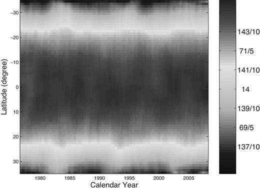
The rotation angular velocities of magnetic fields distributed along latitudes and varying with time, which are obtained by Chu et al. (2010). Latitudes of the Southern hemisphere are negative. The unit shown on the colour bar is |$\text{degrees}\ \text{per day}$|.
Fig. 2 shows four isopleth lines of rotation rates, and the corresponding rotation rates are 14|${^{\circ}_{.}}$|29, 14|${^{\circ}_{.}}$|25, 13|${^{\circ}_{.}}$|10 and 13|${^{\circ}_{.}}$|85 d−1 in turn from low to high latitudes. Any velocity in the figure is the mean of those at the corresponding latitudes of the two hemispheres. Shown also in the figure are the minimum and maximum times of sunspot cycles. As the figure shows, rotation rates on the average seem higher when the magnetic field is weak, indicating that strong magnetic fields should repress solar differential rotation.
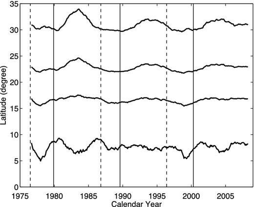
Isopleth lines (bold solid lines) of rotation rates. The corresponding rotation rates are 14|${^{\circ}_{.}}$|29, 14|${^{\circ}_{.}}$|25, 13|${^{\circ}_{.}}$|10 and 13|${^{\circ}_{.}}$|85 d−1 in turn from low to high latitudes. The thin vertical dashed lines indicate the minimum times of sunspot cycles. The thin vertical solid lines indicate the maximum times of sunspot cycles.
Solar-cycle-related variation of solar differential rotation
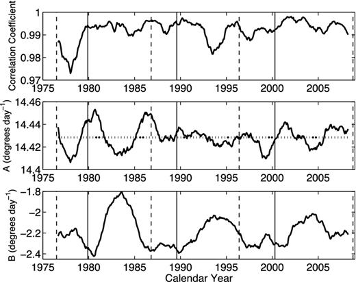
The top panel: the correlation coefficient (bold solid line) of the latitudinal distribution of rotation rates at each CR of the considered time interval fitted by the standard formula of solar differential rotation. The middle panel: the coefficient A (bold solid line) of solar differential rotation. The horizontal dotted lines indicates the mean (14|${^{\circ}_{.}}$|428 d−1) of A. The bottom panel: the coefficient B (bold solid line) of solar differential rotation. The thin vertical dashed lines indicate the minimum times of sunspot cycles. The thin vertical solid lines indicate the maximum times of sunspot cycles.
The latitudinal distribution of rotation rates is fitted by the two-term formula at each of all considered CRs. Fig. 3 shows the correlation coefficient of the formula fitting to the distribution of differential rotation rates along latitudes, and it is larger than 0.97 at each CR. The correlation is thus statistically significant at the 99.99 per cent confidential level. The formula can give a very good fitting at each of all considered CRs. Fig. 3 also shows the obtained coefficients A and B. A peaks around the minimum and maximum times of sunspot cycles, implying the existence of a period of about a half Schwabe cycle in length. The absolute value of B on the average seems larger when the magnetic field is weak, indicating that the magnetic field should repress the differentiation of solar rotation. A special feature of B is that its absolute value clearly decreases and then increases within the descending part of a sunspot cycle.
Values of the coefficient B are averaged for all considered time within the same solar cycle phase relative to the nearest preceding sunspot minimum. As a result, Fig. 4 shows the dependence of the coefficient values on the phase of the solar cycle relative to the nearest preceding sunspot minimum, and their corresponding standard errors. Different solar cycles have different period lengths; thus, also shown in the figure is the dependence of the coefficient values on the phase of the solar cycle relative to the sunspot maximum, and their corresponding standard errors. As the figure displays, the special feature of B can be clearly seen.
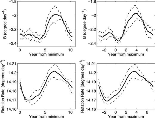
Top-left panel: the dependence (solid line) of values of the coefficient B on the phase of the solar cycle relative to the nearest preceding sunspot minimum, and their corresponding standard errors (dashed lines). Top-right panel: the dependence (solid line) of values of the coefficient B on the phase of the solar cycle relative to sunspot maximum, and their corresponding standard errors (dashed lines). Bottom-left panel: the dependence (solid line) of the latitudinally mean values of rotation rates on the phase of the solar cycle relative to the nearest preceding sunspot minimum, and their corresponding standard errors (dashed lines). Bottom-right panel: the dependence (solid line) of the latitudinally mean values of rotation rates on the phase of the solar cycle relative to sunspot maximum, and their corresponding standard errors (dashed lines).
We calculate the average of rotation rates over latitudes of −35° to 35°, and then the obtained mean values of rotation rates are averaged for all considered time within the same solar cycle phase relative to the nearest preceding sunspot minimum. As a result, Fig. 4 shows the dependence of the latitudinally mean values of rotation rates on the phase of the solar cycle relative to the nearest preceding sunspot minimum, and their corresponding standard errors. Also shown in the figure are the dependences of the latitudinally mean values of rotation rates on the phase of the solar cycle relative to sunspot maximum, and their corresponding standard errors. As the figure displays, the special feature of B can also be clearly seen for the latitudinally mean values of rotation rates.
Periodicity of solar differential rotation
We calculate the autocorrelation coefficient of the coefficient A, varying with relative phase shifts of A with respect to itself, which is shown in Fig. 5. The autocorrelation coefficient peaks to be 0.5812 when phase shift is 74 CRs or 66 months [1 CR = 0.894 month; see Li et al. (2007)], which is statistically significant at the 99.9 per cent confidential level. Thus, there is a period of about 66 months for A. Similarly, we calculate the autocorrelation coefficient of the coefficient B, varying with relative phase shifts, which is also shown in Fig. 5. The autocorrelation coefficient of B peaks to be 0.7931 when phase shift is 141 CRs or 126 months, which is statistically significant at the 99.9 per cent confidential level. Therefore, there is a period of about 126 months for B.
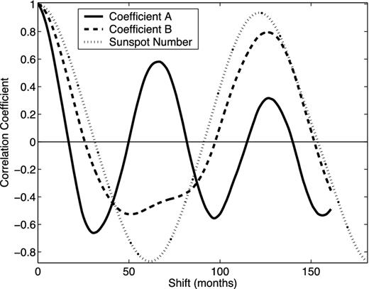
Autocorrelation coefficient of the coefficients A (bold solid line) and B (dashed line) of rotation rates, varying with relative phase shifts of themselves, respectively. The dotted line shows autocorrelation coefficient of monthly mean sunspot, with relative phase shifts of itself.
We calculate the autocorrelation coefficient of monthly mean sunspot numbers at the time interval of 1976 August to 2008 April, varying with phase shifts. Monthly mean sunspot numbers are downloaded from the SIDC's website,1 and they are found to have a period of 121 months, slightly different from that of B.

Comparison of the monthly values (asterisks) of the coefficient B of differential rotations with the original data (solid line).
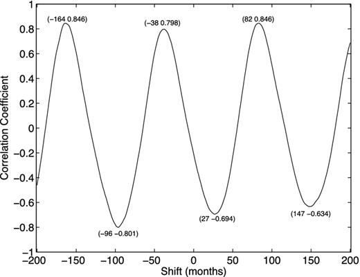
The cross-correlation coefficient of the monthly values of B and the monthly sunspot numbers, varying with shifts of the former versus the latter with backward shifts given minus values. The coordinate values of three peaks and three valleys are given in the figure.
NORTH–SOUTH ASYMMETRY IN SOLAR DIFFERENTIAL ROTATION
It is an interesting and important issue whether the space–time plots of sidereal rotation period show north–south asymmetry or not (Vats & Chandra 2011). Song, Wang & Ma (2005) found that the degree of asymmetry during the minimum of solar activity is higher than that during the maximum of solar activity. Moreover, the change of magnetic flux is always accompanied by a gradual shift of the Northern hemisphere dominance at the ascending time of a solar cycle to the Southern hemisphere dominance at the descending time. Gigolashvili et al. (2005) investigated |$\text{H}{\alpha }$| filaments and found the existence of north–south asymmetry in the chromospheric rotation during solar activity cycles 19–22. With the development of a solar cycle, the north–south asymmetry of solar rotation rate changes, i.e. the differences in the rotation rate should peak at about solar activity maxima, but it changes sign near activity minima from cycle to cycle. Vats & Chandra (2011) showed that asymmetry should appear to change its sign in odd and even activity cycles of the Sun as oscillations with a 22 year period. Here, we will investigate the north–south asymmetry in rotation of the magnetic fields.
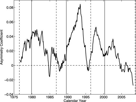
The temporal variation of asymmetry coefficient (thick solid line). The thin vertical dashed/solid lines indicate the minimum/maximum times of sunspot cycles.
CONCLUSIONS AND DISCUSSIONS
The solar differential rotation has a cyclic pattern of change. This pattern can be described as a torsional oscillation, in which the solar rotation is periodically speeded up or slowed down in certain zones of latitude while elsewhere the rotation remains essentially steady (Snodgrass & Howard 1985; Li et al. 2008). The zones of anomalous rotation move on the Sun in a wavelike fashion, keeping pace with and flanking the zones of magnetic activity (LaBonte & Howard 1982; Snodgrass & Howard 1985). The surface torsional pattern and perhaps the magnetic activity as well are only the shadows of another unknown phenomenon occurring within the convection zone (Snodgrass 1987; Li et al. 2008). In this study, the solar-cycle-related variation of solar differential rotation can be explained on the framework of the surface torsional pattern and the magnetic activity as follows.
Brajsa, Ruzdjak & Wohl (2006) investigated solar-cycle-related variations of solar rotation, and they found a higher than average rotation velocity in the minimum of activity. Then they gave a possible interpretation: when magnetic fields are weaker, one can expect a more pronounced differential rotation yielding a higher rotation velocity at low latitudes on an average. Indeed, as Fig. 4 shows, more pronounced differentiation of rotation rates appears at the ascending part of a Schwabe cycle than at the descending part on an average, due to weaker magnetic fields appearing at the ascending part. Strong magnetic fields repress differentiation of solar rotation, so that rotation rates show less pronounced differentiation. But weak magnetic fields seem to just reflect differentiation of rotation rates, and further, weak magnetic fields may more effectively reflect differentiation at low latitudes with high rotation rates than at high latitudes with low rotation rates. As Fig. 4 shows, B may be divided into three parts. Part 1 spans from the start to the fourth year of a Schwabe cycle, the absolute B is approximately a constant or slightly fluctuates (the absolute B seems to slightly increase for which weak magnetic fields more clearly reflect differentiation at low latitudes than at high latitudes). Part 2 spans from the fourth to the seventh year; the absolute B decreases. When solar activity is progressing into this part, sunspots appear at lower and lower latitudes, magnetic fields repress differentiation more and more effectively and differentiation appears less and less conspicuously; thus, the absolute B decreases within this part. Part 3 spans from the seventh year to the end of a Schwabe cycle. Within this part, magnetic fields becoming more and more weak repress differentiation less and less effectively, and sunspots appearing at more and more low latitudes lead to that the differentiation reflected by latitudinal migration should be more and more conspicuous; thus, the absolute B increases.
When solar activity is progressing into a new Schwabe cycle from its former old cycle, more and more sunspots of the new Schwabe cycle appear at high latitudes with relative low rotation rates, and less and less sunspots of the former old Schwabe cycle appear at low latitudes with relative high rotation rates; rotation rate of magnetic fields thus decreases when solar activity transfers to a new Schwabe cycle from its former old cycle (see Fig. 4). From the 1st to the 3.5th of a new Schwabe cycle, rotation rate slightly increases (see Fig. 4) and magnetic fields can more and more clearly reflect differentiation, namely differentiation increases (see Fig. 4), due to the migration of sunspot towards low latitudes. Rotation rates increase from the 3.5th to the 7th year, but decrease from the seventh year to the end of a Schwabe cycle, and the reason why rotation rates vary in such a way is the same as for B given above.
In sum, the solar-cycle-related variation of solar differential rotation is inferred to be the result of both the latitudinal migration of the surface torsional pattern and the repression of strong magnetic activity. This means that measurements of differential rotation should be different at different phase of a Schwabe cycle or/and at different latitudes (different spacial positions of observed objects on the solar disc). That is the main reason why many different results about solar differential rotation exist at the present (Howard 1984; Schroter 1985; Snodgrass 1992; Beck 2000; Paterno 2010).
Both solar magnetic activity and latitudinal migration may be regularized as the Schwabe cycle in the time domain. This is the reason why B basically shows the Schwabe cycle. However, latitudinal migrations of different Schwabe cycles should overlap in the space domain. For example, sunspots of a new Schwabe cycle appear at high latitudes around its minimum time; however, at the same time sunspots of its former Schwabe cycle still appear on the solar disc, but at low latitudes. Sunspots of a new Schwabe cycle at high latitudes and those of its former old cycle at low latitudes give different measurements of differential rotation around the minimum time of the new Schwabe cycle, which should make B to have a slightly different period in length from the Schwabe cycle. The absolute B usually peaks several years after the maximum time of a sunspot activity cycle, that is the reason why the periodicity of B is different in period phase from that of sunspot activity.
The north–south asymmetry in solar rotation is also investigated through fitting the latitudinal distribution of rotation rates of the magnetic fields with a second-order polynomial. The Northern hemisphere is found to rotate faster than the southern at most times of the considered interval. That is to say, the Northern hemisphere should rotate faster in cycles 21–23. The degree of asymmetry during the minimum of solar activity is generally lower than that during the maximum of solar activity.
We thank the anonymous referees for their careful reading of the manuscript and constructive comments which improved the original version of the manuscript. Data of solar differential rotation rates used here are kindly given by Dr. Chu, to whom the authors would like to express their deep thanks. The work is supported by the NSFC under Grants 11273057, 10921303, 11147125 and 11073010, the National Basic Research Program of China (2011CB811406 and 2012CB957801) and the Chinese Academy of Sciences.
