


Abstract
Arecibo observations of the conal triple pulsar B1918+19 at 0.327 and 1.4 GHz are used to analyse its subpulse behaviour in detail. We confirm the presence of three distinct drift modes (A, B, C) plus a disordered mode (N) and show that they follow one another in specific cycles. Interpreting the pulsar's profile as resulting from a sightline traverse which cuts across an outer cone and tangentially grazes an inner cone, we demonstrate that the phase modulation of the inner cone is locked to the amplitude modulation of the outer cone in all the drift modes. The 9 per cent nulls are found to be largely confined to the dominant B and N modes, and, in the N mode, create alternating bunches of nulls and emission in a quasi-periodic manner with an averaged fluctuation rate of about 12 rotation periods (P1). We explore the assumption that the apparent drift is the first-order alias of a faster drift of subbeams equally spaced around the cones. This is shown to imply that the drift modes A, B and C have a common circulation time of 12P1 and differ only in the number of subbeams. This time-scale is on the same order as predicted by the classic E × B drift model of Ruderman & Sutherland and also coincides with the N-mode modulation. We therefore arrive at a picture where the circulation speed remains roughly invariant while the subbeams progressively diminish in number from modes A to B to C, and are then re-established during the N mode. We suggest that aliasing combined with subbeam loss may be responsible for the apparently dramatic changes in drift rates in other pulsars.
INTRODUCTION
Pulsar B1918+19 is a typical ‘slow’ radio pulsar with a stellar-rotation period (P1) of 0.82 s and a spin-down age of 15 Myr. It was one of three apparently conal pulsars with three-peaked profiles whose pulse-sequence (hereafter PS) behaviour was studied at 430 MHz by Hankins & Wolszczan (1987, henceforth HW). These authors identified four distinct modes of emission labelled A, B, C and N – a nomenclature that will also be used here for continuity. The first three modes exhibited drifting subpulses which, together with the fourth ‘disordered’ mode and its embedded null sequences, were found to interact in specific sequences.
In this paper, we exploit the improved signal-to-noise ratio (S/N) of our observations to analyse this pulsar's drift modulation and nulls more thoroughly. A full statistical assessment is given for each mode and type of modal sequence. Recent studies of other similar pulsars have found that nulling is sometimes confined to a specific mode of emission (Redman, Wright & Rankin 2005) or found to have a periodic nature (Herfindal & Rankin 2007, 2009; Rankin & Wright 2007) and we establish here to what degree this is true of B1918+19.
To place our results in a physical, or at least geometric, framework, we consider the context of a rotating subbeam-carousel system (Ruderman & Sutherland 1975, hereafter RS). This has often proved successful in describing drifting subpulses in conal pulsars [e.g. Deshpande & Rankin (1999, 2001, hereafter DR); Bhattacharyya et al. (2007)], and it is now interesting to explore whether the more complex multiple discrete mode patterns of B1918+19 together with their ‘sequence rules’ can be made compatible with such a model.
In Section 2, we describe our observations, and in Section 3, we present what can be inferred about the pulsar's basic emission geometry from its profile and polarization. Section 4 introduces the multiple features in its fluctuation spectra, and Section 5 discusses the profiles and phase patterns of the several modes. Section 6 gives an analysis of nulling statistics, and Section 7 discusses mode sequencing and transitions. In Section 8, we discuss the possibility of aliasing, and Section 9 provides an interpretation of the pulsar's three drift modes in terms of the rotating carousel-beam model, and this is checked against the observationally derived geometry of the pulsar in Section 10. Section 11 summarizes the results and Section 12 draws conclusions.
OBSERVATIONS
The observations were carried out using the 305 metre Arecibo Telescope in Puerto Rico. All of the observations used the upgraded instrument with its Gregorian feed system, 327 MHz (P band) or 1400 MHz (L band) receivers and Wideband Arecibo Pulsar Processors1. The auto- and cross-correlations of the channel voltages produced by receivers connected to orthogonal linearly (circularly, after 2004 October 11 at P band) polarized feeds were three-level sampled. Upon Fourier transforming, some 64 or more channels were synthesized across a 25-MHz bandpass with about a milliperiod sampling time. Each of the Stokes parameters was corrected for interstellar Faraday rotation, various instrumental polarization effects and dispersion. The date, resolution and the length of the observations are listed in Table 1.
Band, resolution and length of Arecibo observations.
| Band | MJD | Resolution | Length |
|---|---|---|---|
| (GHz) | (degrees/sample) | (pulses) | |
| 1.1–1.7 | 527 35 | 0.22 | 1023 |
| 0.327 | 529 42 | 0.22 | 1395 |
| 0.327 | 537 78 | 0.39 | 3946 |
| 1.1–1.7 | 545 41 | 0.36 | 731 |
| Band | MJD | Resolution | Length |
|---|---|---|---|
| (GHz) | (degrees/sample) | (pulses) | |
| 1.1–1.7 | 527 35 | 0.22 | 1023 |
| 0.327 | 529 42 | 0.22 | 1395 |
| 0.327 | 537 78 | 0.39 | 3946 |
| 1.1–1.7 | 545 41 | 0.36 | 731 |
The first two observations were seriously corrupted by interference.
PROFILE GEOMETRY
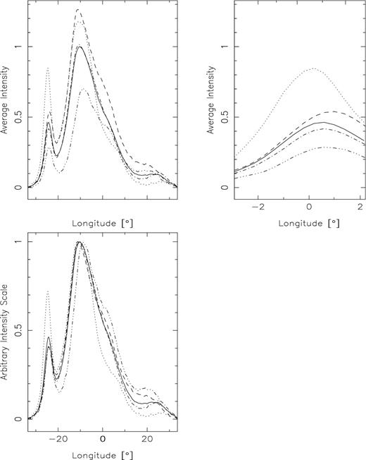
The B1918+19 polarization profile and PPA histogram, shown in Fig. 1, consists essentially of four components, a distinct leading component, a central ‘main’ component exhibiting a clear shoulder, plus a weak trailing component some 35° of longitude after the peak. Its profile has therefore been placed in the relatively uncommon conal quadruple category (Rankin 1983, 1993a,b; hereafter ET I, ET VIa,b), and we now know that some other such stars also have highly asymmetric profiles (e.g. J1819+1305; see Rankin & Wright 2008). The available profiles of B1918+19 (i.e. Gould & Lyne 1998; Hankins & Rankin 2008) suggest that it becomes more symmetric at higher frequencies, but no published profile at a frequency higher than 1.6 GHz seems to exist. The relative intensity of the first component at metre wavelengths also seems to vary considerably, but as we will see below, this is probably due to the specific population of modes present in the average.
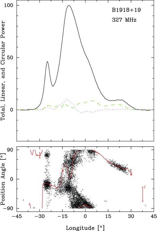
Average profile of B1918+19 computed from the long 327-MHz observation. Notice the leading and compound primary components and the relatively weak trailing component. The top panel gives the total intensity (Stokes I, solid curve), the total linear (Stokes L (=|$\sqrt{Q^2+U^2}$|), dashed green) and the circular polarization (Stokes V, dotted magenta). The lower panel PPA (=|${1\over 2}\tan ^{-1}(U/Q)$|) histogram corresponds to those samples having PPA errors smaller than 10° with the average PPA traverse (red curve) overplotted. The longitude origin is taken about halfway between the outer conal component pair.
The aggregate linear polarization L never exceeds about 10 per cent in Fig. 1, but the geometric polarization angle (hereafter PPA) sweep rate can be reliably traced once the effects of two modal ‘flips’ are resolved. The PPA then makes a total traverse of about −120°, and the central rate R is some −3.2°/°. Despite the then limited information, B1918+19's basic emission geometry seems to have been computed almost correctly in ET VIa,b: its respective inner and outer cones have half-power, 1-GHz widths of 20| ${.\!\!\!\!\!\!^{\circ}}$|5 and 51| ${.\!\!\!\!\!\!^{\circ}}$|3, respectively. Its magnetic latitude α and sightline impact angle β are then 14° and −4| ${.\!\!\!\!\!\!^{\circ}}$|3 for a poleward traverse across its emission cones (or 11° and +3| ${.\!\!\!\!\!\!^{\circ}}$|4 for an equatorward traverse, although this model fits the inner/outer conal dimensions less successfully). In either case, the sightline encounters the inner cone tangentially (with β/ρ ∼ 0.9, where ρ is the outer half-power conal radius) and the outer cone much more centrally (−0.65/0.52) – confirming the earlier qualitative interpretation of the star's double-conal emission geometry. Moreover, the prominent polarization-modal activity on the profile edges seems to confirm that we are observing emission from the full widths of the cones. Note, though, that the PPA distribution in the leading half of the central component consists of a set of ‘patches’ rather than two PPA tracks.
PS MODULATION
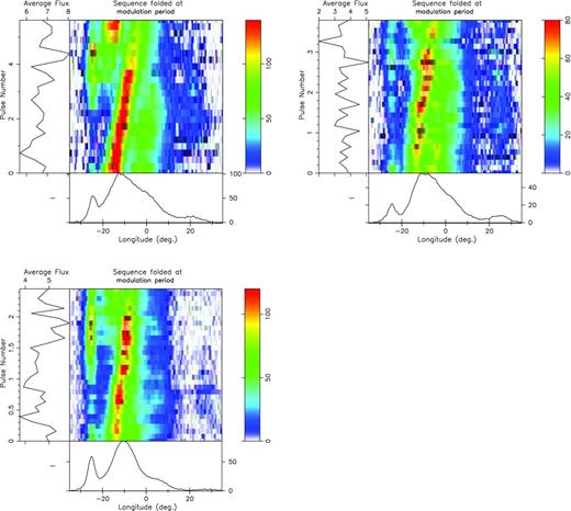
The two extracts from our longer 327-MHz observation presented in Fig. 2 show the essential features of B1918+19's single pulse behaviour. Using the nomenclature of HW, the 340 pulses on the left show several examples of a relatively slow drift pattern (A) changing rapidly into a faster mode (B), which is then followed by an irregular null-rich sequence (N). The same number of pulses in the right-hand panel show a typical long sequence of the fastest mode (C) interrupted by a relatively long null. The exceptional S/N of the whole observation enables us to analyse these basic features in some detail.
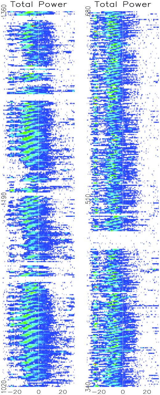
Two single pulse plots, each of 340 consecutive pulses from the same observation of B1918+19, separated by about 1000 pulses. Left: several sequences of mode A transforming into mode B interposed by the null-rich irregular N mode. Note the nulls creating an approximately 85-pulse periodicity. Right: an extended sequence of the fast mode C interrupted by an extended null. Longitude scale in degrees.
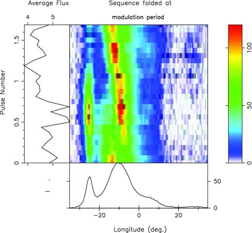
The longitude- and harmonic-resolved fluctuation spectra (hereafter lrf and hrf) of the entire 327-MHz observation are given in Figs 3 and 4. In the lrf spectra, four clear features are visible, in addition to a prominent low-frequency feature. The periodicities corresponding to the A, B and C modes, which represent the vertical spacing of the driftbands and are conventionally denoted as P3, are very evident, with centroid values only slightly different from those of HW. The A mode has a P3 of 6.06P1 (=1/0.165 cycles/P1; hereafter c/P1; 5.9P1 in HW); the B mode a P3 of 3.80P1 (=1/0.263 c/P1; 3.85P1 in HW); and the C mode a P3 of 2.45P1 (=1/0.408 c/P1; 2.5P1 in HW). Substantial scatter about these values is visible in Fig. 3 (especially in the B mode), but we will show below that they are often nearly coherent in particular sections of the PS. Note also that the periodicities corresponding to these three modes are found not only in the central component of the integrated profile, but also in the outer component pair. Significantly, the A and B modes modulate both the leading and trailing components, although on the trailing edges at differing longitudes. The C-mode modulation is also prominent in the leading component but invisible in the trailing one, where the intensity of this mode is anyway very weak.2
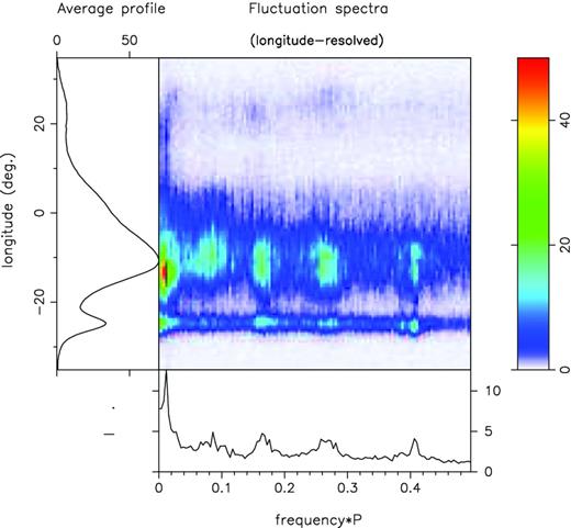
Longitude-resolved fluctuation power spectra for the 327-MHz observation of B1918+19 on MJD 539 67 (main panel, per the colour scale at the right), plotted against the total power profile (left-hand panel) with the integral spectrum in the bottom panel. Five different features are seen in these spectra: The three highest frequency features correspond to the A, B and C modes identified by HW with P3 values of 5.8, 3.9 and 2.5 cycles/P1. In addition, two lower frequency periodicities are present, a well defined one corresponding to a P3 value of some 85P1 and a broad response at about 12P1. Note that the 2.5P1, 3.9P1 and 5.8P1 features all modulate outer regions of the outer cone to some degree although the 2.5P1 feature is not detected in the trailing component. Finally, the low-frequency feature modulates the entire profile, whereas the 12P1 modulation affects the central inner-cone region only.
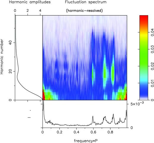
Harmonic-resolved fluctuation spectrum for the same observations as in Fig. 3 (main panel, per the colour scale at the right). Rather dramatically, this shows that HW's three features are all phase-modulated. The low-frequency response, by contrast, is a mixture of phase and amplitude modulation, and the 12P1 response appears to represent mostly amplitude modulation. This distinction can also be seen in the main panel where the low-frequency modulation is carried by smaller numbered Fourier harmonics than HW's drift modulation, which seem to peak about number 18 or so. In the central panel, the amplitude scale has been compressed by a factor of 3 to accentuate the three phase-modulated periodicities.
The A–C features also appear prominently in the hrf spectrum of Fig. 4, but here almost exclusively at fluctuation frequencies between about 0.6 and 0.85 c/P1. The main panel shows clearly that these periodicities represent phase modulations corresponding to sets of drifting subpulses separated by P2 ∼ 20° (=360°/18) and their presence at frequencies over 0.5 indicate that the apparent drift is towards increasing longitudes. In itself the hrf spectrum cannot determine the true subpulse drift, i.e. whether or not the observed drift pattern is aliased (in which case the intrinsic drift would be towards decreasing longitudes). This point is further discussed below.
This new 12-P1 periodicity may well arise within the irregular null-rich N mode, which is known to have a peak intensity at a slightly later longitude than the other modes and to be characterized by a weak first component. This will be investigated in a later section, but it can be seen in the left-hand PS of Fig. 2 that intensity fluctuations on roughly this time-scale occur between the A and B modal sequences. It is interesting to note – not for the first time in pulsars with multiple drift patterns – that the periodicities of this pulsar appear to have ‘harmonic’ properties: the new periodicity (12.0P1) is practically twice that of the A mode (6.06P1), which in turn is about three-halves of the mean value of the B mode (3.80P1) and five-halves of the C-mode periodicity (2.45P1).
Finally, the low-frequency feature in the two spectra – mentioned in passing by HW and attributed to ‘deep nulls’ – has its peak before the profile peak and is prominent across nearly the entire profile. A striking example of how this feature is generated in the PS can be seen in the left of Fig. 2, where the 340 pulses are divided into 4 roughly equal sections by the intrusion of the N mode. However, in the PS as a whole this represents more of a characteristic time-scale rather than a periodicity. In the hrf spectrum (Fig. 4), the feature interestingly reveals itself to be an admixture of amplitude and phase modulation – the latter counter to that of the A–C modes and focused on a narrow band of longitude preceding the profile peak by about 3°. (NB: a similar feature was found in J1819+1305 in an earlier paper.)
As suggested by Fig. 2, these last two periodicities (12P1 and 85P1) do appear to be null related. A number of the nulling pulsars exhibit such low-frequency fluctuation spectral features, and when the PS modulation is quelled by substituting a scaled-down profile for the pulses and zeroes for the nulls, the periodicities often persist (Herfindal & Rankin 2007, 2009). The latter study shows that this is so for B1918+19 as well; three different periodicities appear to be present in the pulsar's null sequence: a seemingly harmonically related pair at 85 ± 14 and 43 ± 4P1 as well as the roughly 12P1 one.
DISTINGUISHING THE MODES
Using colour displays such as those used in Fig. 2, we inspected the entire long 327-MHz PS to identify sections exhibiting the A, B and C modes, usually on the basis of their characteristic periodicity. Mode N was identified by the absence of a clear drift, often accompanied by weakness in the first component.
By far the most common mode was B (1896 pulses or 48 per cent), followed by N (847 pulses or 21.5 per cent), A (662 pulses or 17 per cent) and C (541 pulses or 14 per cent). However, these statistics disguise considerable discrepancies in the typical sequence lengths of the modes: while all C-mode pulses occurred in just 4 long null-free sequences, averaging 135 pulses in length, the 36 N-mode PSs averaged only 23.5 pulses, and the A- and B-mode PSs averaged 35 and 53 pulses, respectively.
By segregating the pulses appropriately a partial-average profile was computed for each mode. Fig. 5 (top left) shows the profiles weighted according to their relative average intensities. Note that the average intensities of the A- and C-mode pulses are clearly stronger than those of the B and N modes. This differs slightly from the conclusion of HW, who found, after selecting 300 bright pulses from each mode (at 430 MHz), that the average intensities of all the modes were more comparable. Their result can be reconciled with ours if, as seems likely, the weaker pulses (including nulls) tend to occur in the B or N modes. Particularly striking in both ours and HW's results is the enhanced intensity of the leading component in the C mode, which is about double its average strength in the other modes. The first component peak appears about 1° earlier in the C mode than in the A mode, with those of B and N modes falling in between (top-right panel).
Partial profiles for the several modes as well as the average profile: (top left) normalized to their relative intensities, (top right) leading component detail and (bottom) scaled to the peak intensities. Total average profile (solid line) as well as the A (dashed), B (dash–dotted), C (dotted) and N (dash–triple dotted line) modes. Note that the leading component of the C mode is significantly larger than in any other mode, whereas its trailing component is much smaller. It also peaks about 1° earlier than the A mode, while the B mode peaks somewhere between. Similarly, the normalized profiles (bottom) clearly show the shift of the peak of the N mode as well as the curtailed trailing edge of the C mode.
By contrast, Fig. 5 (bottom) shows the same partial profiles, but now normalized to the amplitude of the total average profile peak. This exhibits the attenuated latter half of the C-mode profile: there is no ‘hump’ on the trailing edge of its main component, and its weak fourth component all but vanishes. The fourth component is strongest in the A mode and appears at a closer longitude to the main pulse than the fourth component of the B mode. The plot also enables comparison with a similar graph in HW (their fig. 4). The results are broadly compatible, but our profiles show a much smaller relative intensity in the region between the leading and main profile components, reflecting the much better resolution of our observations.
HW also found that the peak in the N mode falls about 3° later than in other modes, whereas our results do indeed show a peak shift, but only of about 2° (Fig. 5, bottom-left panel). A possible explanation for these discrepancies can be a shift in the centroid of the drifting pulses towards earlier longitudes as they become more intense.
Although the modal partial profiles in Fig. 5 all have distinguishing properties, the underlying subpulse configuration in the three drifting modes A, B and C is nearly identical. The three panels of Fig. 6 display selected intervals folded at the appropriate P3 values for modes A (top left), B (top right) and C (bottom), respectively. In all three modes, the drift bands appear to have a similar longitudinal separation (P2), a point also noted by HW. Most striking, however, is the phase-correlated behaviour of the leading and main-component emission patterns. The leading component does not drift but instead modulates its intensity at the same P3 as the drift in the main component (evident in the fluctuation spectra of Figs 3 and 4).
Drift-modal sequences folded at their respective P3 values: A (top left, pulses 2404–2458); B (top right, pulses 2600–2800); and C (bottom, pulses 481–735). Note the strong similarity of all three patterns, including the relative phase positions of the leading and trailing components. Thus, whether aliased or not, in each mode the pulsar is executing virtually the same pattern at a different speed.
Note that the phase of the subpulse emission in the leading component is correlated with the drift patterns in the main components in a similar manner in all three modes. Although the emission level of the leading component varies from mode to mode, in each case it is strongest as or just before the drift band reappears at the leading edge of the main component. A similar correlation is also discernible between the main and trailing components. In the A mode (Fig. 6, top left), there is evidence of an emission peak at the longitude of the trailing component of the main pulse. Interestingly, this peak does not occur at the same phase as that in the leading component, but follows it by about 4.5P1 or 0.65 in phase. There is also a hint of this peak at the same relative phase in the B-mode fold of Fig. 6, top right, lending an inverse-reflection symmetry to the modulation pattern [noted also between the two halves of the emission pattern of B0834+06 (Rankin & Wright 2007) and in B0818−41, where the phase shift is close to 0.5 (Bhattacharyya et al. (2009)].
Thus, B1918+19 joins the relatively short list of pulsars both classified as having double-cone structure and whose single-pulse patterns are phase locked (B1237+25, B0826−34, B0818−41, B1039−19; see Srostlik & Rankin 2005; Gupta et al. 2004; Bhattacharyya et al. 2007, 2011, respectively). However, as pointed out by Bhattacharyya, Gupta & Gil (2009), there are as yet no examples where phase locking is not present in double-cone pulsars. In B1918+19, we can additionally see that the phase locking survives multiple drift-mode changes. The similarity of the pattern in all three modes suggests that the emission processes are simply executing a very similar pattern at three different speeds and demonstrates that all components interact as a single physical system, thus pointing to a common geometry and a common emission process.
QUASI-PERIODIC NULL PATTERNS
The excellent S/N ratio of the PSs from the upgraded Arecibo instrument enabled us to study B1918+19's nulling properties in detail for the first time. Fig. 7 gives the pulse–intensity histogram for the 327-MHz 3946-length PS. It shows a population of weak pulses around zero energy that is distinct from the low-energy tail of the primary intensity distribution. This suggested a conservative definition of a null as having an intensity less than the minimum in the distribution, which occurred at 0.18 〈I〉. Using the indicated threshold at 0.18 〈I〉, the null fraction was found to be ∼8.9 per cent or 350 pulses.
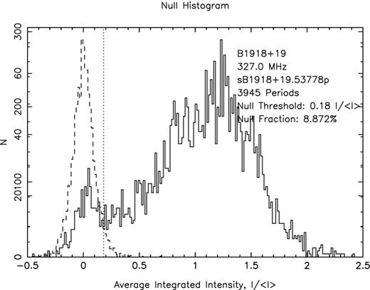
Pulse–intensity histogram (solid curve) for the long 327-MHz observation of B1918+19 and a corresponding off-pulse noise window (dashed curve). The vertical dotted line indicates a plausible null threshold at 0.18 〈I〉 (see the text). Some 21 pulses were omitted from the distribution due to bad baselines.
A histogram of null lengths in Fig. 8 (top) was computed to investigate their statistical properties. Its most obvious feature is the peak of 80 isolated null pulses. If the 350 nulls had appeared randomly among the 3946 pulses with an 8.9 per cent chance in each pulse, the expected number of isolated nulls would have been some 320. The non-randomness of the distribution is then obvious from the massive excess of null pulses occurring in bunches longer than one pulse. It is also reflected in the highly negative ‘overclustered’ Runs-Test value (see Redman & Rankin 2008).
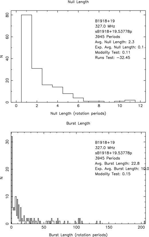
Histograms of null (top) and burst (bottom) lengths.
Visual study of the PSs (see Fig. 2) strongly suggests that the nulls are closely associated with the N mode, occurring predominantly before, during, after or within it – so it remains possible that nulls are appearing randomly, but confined to this mode of emission. If we postulate that all the nulls occur with this set of 847 N-mode pulses – where its null fraction would then be 41 per cent (=350/847) – we could expect some 82 single nulls, very close indeed to the number that we observe. The null-length distribution is also statistically overweight in relatively long (>3) contiguous nulls. In particular, the observed 3 occurrences of 10 and 11 consecutive nulls remain highly improbable. It seems an inescapable conclusion that the nulls in this pulsar do have an intrinsic bunching tendency such that once a null pulse occurs, the chance of a null in the next pulse is enhanced.
We also noted that groups of null pulses often precede and follow a typical 6–10 pulse burst of emission, even once during the B mode in an apparent interruption of that mode. In Fig. 8 (bottom), a histogram of the emission-burst lengths indeed reveals a distinct peak around 6–10 pulses, which can be attributed to this emission bunching. (Also visible is a statistical excess of 1P1 bursts, reflecting emission ‘flickering’ within sequences of nulls.) Thus, nulls not only tend to occur in bunches, but those bunches appear in a quasi-periodic manner – obviously in the N mode and often during transitions between modes (see the next section). We have already noted (e.g. Fig. 5) that the N-mode emission is characterized by weak leading-component emission and a slight shift in the main peak towards later longitudes (see Fig. 2). These are precisely the properties shared by the unexpected 12P1 feature in the fluctuation spectra of Figs 3 and 4, and we are therefore confident that the quasi-periodic nulls associated with the N mode are responsible for that feature.
MODAL SEQUENCES AND TRANSITIONS
Studies of the few pulsars with multiple drift modes (Huguenin, Taylor & Troland 1970; Wright & Fowler 1981; Redman et al. 2005) have shown that the modes occur in sequences of increasing drift rate. HW found this to be true for pulsar B1918+19 also, and determined, more specifically, that it exhibits two characteristic modal sequence patterns: null → N → A → B → N → null, and null → C → null.
We found that these two patterns do indeed occur, and they are illustrated in Fig. 2, with several examples of the first type shown in the left-hand panel and the C-mode-dominated pattern on the right. However, they are not the only patterns this pulsar exhibits. In particular, we noted frequent examples of the B and N modes being both preceded and followed by null bunches (see Section 6), and there was one possible instance of a null → B → C → null sequence. The A mode never seems to null and is invariably followed by the B mode. It seems that in all cases a general rule is preserved that mode sequences are always from slower to faster observed drift and are concluded by the N mode or nulls. Nevertheless, the C mode, while not violating the rule, tends to occur in long PSs with little or no intrusion from other modes, and no examples of A → B → C were found.
In this picture, the N mode (together with its accompanying nulls) acts as a kind of reset, during which the acceleration of the drift rate ends and the subpulse pattern prepares to recommence at a slower rate, be it A, B or sometimes C. It is accompanied by a fading of the leading component and a slight shift of the central intensity to later longitudes. Interestingly, we found one ‘reset sequence where the leading component did remain strong and gave the emission a periodicity of about 12P1 punctuated by nulls at this periodicity. This sequence looked more like a fourth slow drift mode than simply a disordered N mode and was followed by the A mode, thus being consistent with the rule of incrementally increasing drift rates. Interestingly, the role of nulls as agents of ‘reset is not new: Bhattacharyya, Gupta & Gil (2010) noted this effect in B0818−41, a pulsar with variable drift, though not with multiple modes.
HW comment that the modal transitions may be more gradual than those found in other pulsars (such as B0031−07). We would suggest that this may not be so. Initial visual inspection of the drift bands seems to indicate that some A → B transitions may be discrete rather than continuous, while others may actually ‘overshoot’ the B mode, with the drift rate starting in the slow A mode, then quickly accelerating to even become slightly faster than the B mode, only to settle down to the typical B-mode drift rate within a few pulses. In the left-hand panel of Fig. 2, it is also evident that each A → B sequence has increasing then diminishing intensity, giving the mode change the sense of evolution. This is not seen in the purely C-mode sequence shown in the right-hand panel, suggesting that the two types of sequences are of different character, with the latter more stable than the first.
THE POSSIBILITY OF ALIASING
In the previous section, we have analysed only the observed drift rate changes and, in common with most observers referenced earlier, perhaps tacitly assumed that the observed rates are the true rate. In this section, we analyse the consequences of challenging this assumption.
When observing pulsars we sample the emission once every rotation period. If this sampling rate happens to be frequent compared with the time-scales of intrinsic changes in the emission, then we can obtain an adequate description of the phenomenon we are seeking to understand. Assuming this to be true for B1918+19, we may interpret the observed drift bands as corresponding to individual subbeams gradually moving across the observer's line of sight at the observed drift rate D (the amount of longitude phase the subbeam drifts in one pulse). The repetition rate P3 of this pattern is then P2/D and is significantly larger than P1, the sampling rate. However, from the lrf of Fig. 3, and above all from the PS in Fig. 2, it is clear that P3 switches between several distinct values. Since P2 remains at roughly the same value, the conclusion must be that mode changes arise from changes in the subbeam drift rate D, which more than doubles as P3 reduces from mode A to mode C.
This is a perfectly self-consistent way of interpreting our observation. However, any physical model must then explain why the subbeams change their intrinsic drift speed so drastically, and why these speeds always select from the same values. In the framework of the carousel model (Ruderman & Sutherland 1975; DR; Gil & Sendyk 2003), there is no suggestion as to how this can be achieved and why multiple fixed drift rates might be expected.
Here, we see the same C-mode PS of Fig. 6 (bottom) folded at the assumed unaliased |$P^{\prime }_{3}$| of 1/.59 = 1.69P1. Note that now the drift is faster and from the trailing to the leading edge, and is equivalent to a fluctuation frequency of −0.41 c/P1. The A and B modes can also be folded as above with the appropriate values of |$P^{\prime }_3$| shown in Table 2, also giving reversed drift directions and similarity in pattern.
The P3 values are well in excess of the |$P^{\prime }_3$| values which generate them because D′ and P2 are close in value, yielding a small denominator (P2 − D′) in equation (1). Hence, the observed, apparently large reductions in P3 which occur at a mode change require only a small change in D′, or a small change in P2, or both. Unlike the case where P3 is assumed to reflect the true drift, an aliased mode change in P3 can be observed even if the drift rate remains unchanged, requiring only a small, perhaps observationally imperceptible, change in P2. This would suggest that a physical account of a mode change need not be as drastic as under the non-aliasing assumption. It may be simply the result of somewhat greater or less bunching in the subbeams. However, the question as to why the system always returns to the same discrete modes remains unanswered.
CAROUSEL-MODEL CONFIGURATION
The carousel model assumes that the observed subbeams with their corresponding P2 and D′ reflect the circulation of a number (n) of sparks about the pulsar's magnetic axis. Their observed properties will depend on frequency and height of the emission, but the values of P3, |$P^{\prime }_3$| and n should be frequency and height invariant.
Note that this is almost precisely what can be seen in Fig. 4, where fluctuations peaking near 0.83, 0.75 and 0.58 c/P1 are evident. One can even see vestiges of a weak periodicity at 0.67 c/P1 that corresponds to a carousel with eight subbeams, and although we have never identified any stable PS with these properties, it does seem to be present as a transitional structure when the A mode sometimes ‘overshoots’ the B and then resets to the B.
The role of the N mode is interesting. We have noted earlier that this mode is accompanied by a periodicity with P3 ≈ 12P1, partly generated by repeated null bunches embedded in the N mode. Can it be a coincidence that this is precisely the value deduced by separate arguments for the fixed circulation period? There are two ways this might happen. First, according to equation (4), this value would be consistent with a circulation of |$\hat{P}_3\approx 12 P_1$| – but with exactly n = 11 subbeams. Thus, the sequence N → A → B → N corresponds to a one-by-one reduction in subbeams from 11 to 9 and re-set. Extrapolating further, 12 subbeams would, through aliasing, formally produce an infinite P3 – i.e. sustained non-drifting emission with a narrow P2 during the relatively short duration of the often irregular N mode. Thus, the sequence may even be argued as starting at n = 12 (see Table 2).
A second – or an additional – way of explaining the N-mode periodicity would be to speculate that the subbeam system breaks up as n reduces below the C-mode value of 7. At low values of n the subbeam separation P2 would rapidly grow to twice or more than the values in the A, B and C modes (see Table 2), so that when n equals, say, 3 or 4 the observer would see a flickering or a series of pulses with deep nulls between the subbeams, depending on the width of the subbeams. Once the system has degenerated, the circulating system might just be partly null and partly irregularly located beams, so that in the N mode we see the circulation time directly. Thus, the N mode could be explained as both being the ending and the beginning of the modal cycles, emphasizing its role as the mode during which the cycles are reset.
Obviously missing in the sequence is the case of n = 8 subbeams, where a P3 of 3.0P1 would be expected. However, we note that there is no clear evidence of the B mode progressing directly to the C mode, suggesting that the C mode arises under separate circumstances and is observed to be steadier than the A and B modes (Fig. 2). The reason for the stability of the C mode is suggested by the form of equation (4): when n is close to |$\hat{P}_3\approx 12 P_1$|, as it is in modes A and B, small modulations in |$\hat{P}_3$| may cause observable modulations in P3, but when n is smaller (7), as in mode C, modulations in the drift rate will not significantly modulate the aliased P3.
A summary of this picture is given in Table 2. The observed values of P3, assumed to be first-order aliased, are shown without parentheses, together with their inferred true drift repetition rates |$P^{\prime }_3$| and inferred circulation times |$\hat{P}_3$|. The near-invariant circulation time of 12P1 is then assumed to deduce the expected P3 and |$P^{\prime }_3$| for other integral values of n, and these are shown in parentheses. In the last column, we give the angular spark separation for each n. Note how these increase weakly for high n but widen dramatically for small n.
Carousel-model expectations of the circulation time (|$\hat{P}_3$|) for different n assuming P3 is the first-order alias of |$P^{\prime }_3$|. Comparisons corresponding to observed P3 values are shown bold and without parentheses.
| n | P3 | |$P^{\prime }_3$| | |$\hat{P}_3$| | 360/n |
|---|---|---|---|---|
| (P1) | (P1) | (P1) | (°) | |
| 12 | (∞) | (1.00) | (12.00) | 30 |
| 11 | 12.0 | 1.09 | 12.00 | 32.8 |
| 10 | 6.06 | 1.20 | 12.00 | 36 |
| 9 | 3.8 | 1.36 | 12.24 | 40 |
| 8 | (3.0) | (1.50) | (12.00) | 42.5 |
| 7 | 2.45 | 1.69 | 11.83 | 51.5 |
| 6 | (2.00) | (2.00) | (12.00) | 60 |
| 3 | (1.33) | (4.00) | (12.00) | 120 |
Finally, if B1918+19's circulation time |$\hat{P}_3$| is about 12P1, and the N, A, B and C modes reflect carousel configurations with 11, 10, 9 and 7 subbeams, respectively, then how are we to understand the 85P1 fluctuation feature found in the lrf of in Fig. 3? As mentioned above, this feature is null associated, and while from the hrf of Fig. 4 it seems to be a combination of amplitude and phase modulation, it is carried by such small Fourier components that it must be a modulation of the entire profile. Interesting also is the fact that one sees little of this feature in the analysis of shorter PSs. The A-mode PSs are too short, and those in the C mode do not seem to null. Rather it is the B and N modes that are typically punctuated by nulls, and the former are usually rather long, averaging 53 pulses, while the N mode averages 23.5 pulses.
What we therefore believe, and what is evident from our PS in the left-hand panel of Fig. 2, is that this feature is associated with the full modal cycle of N → A → B → N, which tends to start and end with nulls. Similarly, the 43P1 feature arises from the shorter and less frequent N → B → N cycle. The cycle involving the C mode is of a different character and never exhibits this feature.
EMISSION GEOMETRY
In the previous section, it has been argued on purely mathematical grounds that the apparent repetition patterns of B1918+19's emission can arise from first-order aliasing of equally spaced circulating subbeams. Assuming the circulation rate to be unvarying, it was possible to show that each of the observed drift rates corresponded to a different integral number of subbeams, and hence to a specific angular spacing of those subbeams (Table 2).
We must now ask whether the angular spacing generated at the pulsar's polar cap for each mode is compatible with the spacing P2 of the emission beams at our observing frequency. This spacing is only relevant for drifting subpulses, implying here that it must be evaluated for the inner cone in the central part of the profile, not the outer conal components on the profile edges. And, of course, we are interested in the values for each of the three drifting modes, A, B and C.
Measuring P2 accurately is never trivial, and B1918+19 entails several further complications: first, the always short A-mode episodes introduce one kind of difficulty and the incomplete trailing part of the main component in the C mode another. With 20/20 hindsight, we can see that HW's P2 values in their table are inconsistent, and we will argue that they are least correct with their C-mode value. HW determined their values directly by measuring the intervals between subpulses. Another method uses the phase ramp of the lrf spectra, and we give such a diagram for the C mode in Fig. 10. There it can be seen both that the fluctuation power is virtually absent under the trailing part of the profile, but in the immediately adjacent leading part, the slope is such that a 360° excursion would correspond to about 18°–20° of longitude. This gives an estimate of the C-mode P2, but a poor one owing to the restricted longitude range of the modulation. Similar phase diagrams for short B- and A-mode PSs (pulses 2459–2520 and the 55 A-mode pulses in Fig. 6) provide better estimates, suggesting P2 values of some 14°–15° and 13°± 2°, corresponding to 33 and 30 ± 5 ms, respectively (40 ± 4 and 33 ± 3 ms in HW).
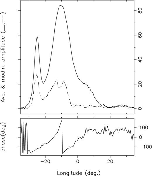
Modulation phase diagram for the C-mode PS in Fig. 9.
P2 values can also be estimated from the hrf spectra, and we computed an hrf with the longitude restricted to the central component (not shown). This did not seem to significantly affect the three features corresponding to the drift modes. However, taking the hrf of the relatively long C-mode PS (Fig. 11), we can see that the primary modulation is associated with the Fourier component peaking at about 20 (its harmonic very clearly peaks about component 40); therefore, P2 here is very near 360°/20 or 18° or 41 ms (34 ± 2 ms in HW). We found it difficult to measure the A- and B-mode P2 values by this method, and the problem is discernible in Fig. 4. The harmonic numbers carrying the B and A mode are clearly smaller as can be judged from their harmonics, but the peaks themselves are too broadened and conflated to give any reliable estimate.
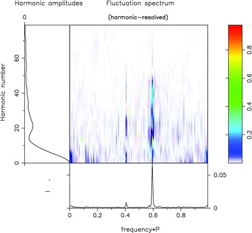
The hrf for the C-mode PS in Fig. 6. Note that the drift modulation is carried by Fourier components around or just greater than 20 and that a second harmonic is discernible. These imply that P2 for this mode is ≈360°/20 = 18°.
The above P2 values are given in Table 3, and we can use these values for each mode, together with the inferred geometry of the pulsar with respect to us, to compute what kind of carousel subbeam system underlies them. Starting with the profile geometry in Section 3 above, it is of importance here that the deduced α and β values square with the central PPA rate R [= sin α/sin β] of −3| ${.\!\!\!\!\!\!^{\circ}}$|2/°. The circumstance that this pulsar has an inside (poleward) sightline traverse (as does B0943+10) is also quite clear from the profile geometry and linear character of the star's PPA traverse.
Geometrically deduced values of n for modes A, B and C.
| α | β | P2 | η | n |
|---|---|---|---|---|
| (°) | (°) | (°) | (°) | |
| 13.7 | −4.2 | 13 | 36.1 | 10.0 |
| – | – | 14.5 | 40.4 | 8.9 |
| – | – | (16) | (44.7) | (8.0) |
| – | – | 18 | 50.6 | 7.0 |
| α | β | P2 | η | n |
|---|---|---|---|---|
| (°) | (°) | (°) | (°) | |
| 13.7 | −4.2 | 13 | 36.1 | 10.0 |
| – | – | 14.5 | 40.4 | 8.9 |
| – | – | (16) | (44.7) | (8.0) |
| – | – | 18 | 50.6 | 7.0 |
The point is that P2 subtends a particular magnetic polar longitude η, which in turn can be used to estimate the subbeam number. DR give such a relation as their equation 3, but Gupta et al.'s equation 6 is more accurate because it distinguishes the conal edges from the subbeam path within the cone. We used a version of this relation sin η = sin (α + β)sin P2/sin Γ where the subbeam path η is 0| ${.\!\!\!\!\!\!^{\circ}}$|8 interior to the outside conal half power point. Note that this value closely reflects the difference between the outer half-power and peak conal radii in the models of ET VIa,b and Gil & Sendyk (2000). Therefore, in our case, β is negative, so the peak subbeam track has a magnetic polar colatitude of |β + 0| ${.\!\!\!\!\!\!^{\circ}}$|8| or 3| ${.\!\!\!\!\!\!^{\circ}}$|4. Then, the subbeam number n can be estimated as 360°/n. These simple computations are assembled in Table 3, where it can be confirmed that the derived subbeam numbers are near integral and are fully compatible with the integers 10, 9 and 7 for the A, B and C configurations, respectively, in Table 2. As a check, one can also carry out these computations for a positive (equatorward) sightline geometry, and the resulting η values are roughly twice as large, implying a very small number of subbeams, demonstrating that this sightline would be incorrect.
SUMMARY OF RESULTS
In 1987, Hankins & Wolszczan carried out the first analysis of the properties of B1918+19, attracted by its entirely conal triple (cT) profile and the added opportunities this configuration presents to investigate the relationships of emission in its inner and outer cones. Using Arecibo PSs, they were able to identify the four basic single-pulse modes of emission (A, B, C and N) and noted specific cyclic relationships between these modes.
Here, with the advantage of more recent data from the same telescope but at a slightly lower observing frequency, we explore the geometry of the pulsar and refine and add to the known single pulse repetition patterns. Further, we propose a possible carousel configuration present at the polar cap which may explain the mode changes with a simple idea. Before discussing this model in the next section, it is useful to summarize our observational results:
B1918+19 has integrated properties common to many pulsars: it has a cT profile with very nearly the usual angular dimensions for its inner and outer cones – half-power conal radii ρ at 1 GHz of 4| ${.\!\!\!\!\!\!^{\circ}}$|1 and 6| ${.\!\!\!\!\!\!^{\circ}}$|5 – as computed originally in ET VIa,b. Its integrated polarization properties suggest that the magnetic latitude α and sightline impact angle β are some 13| ${.\!\!\!\!\!\!^{\circ}}$|7 and −4| ${.\!\!\!\!\!\!^{\circ}}$|2, respectively, such that its inside (poleward) sightline traverse cuts its inner cone tangentially (β/ρ ∼ −0.90) and outer cone obliquely (β/ρ ∼ −0.65)
The profile exhibits leading/trailing asymmetry of two types: the leading (outer) conal component is much stronger than the trailing one and the leading part of the main (inner cone) component is stronger than the trailing part. This asymmetry is least marked in the N mode, and becomes stronger in the A and B as well as the C mode – wherein trailing portions of the profile nearly vanish.
As HW found, the star's PSs exhibit three highly discrete drifting modes, A, B and C, as well as a non-drifting N mode, However, the pulsar exhibits five prominent fluctuation features, three corresponding to the A, B and C drift modes with P3 values near 6.0, 4.0 and 2.5P1, and two null-related features at about 12 and 85P1.
About 9 per cent of the pulses are ‘nulls’ but these nulls are distributed in a highly non-random manner, evidenced by the substantial fraction of nulls with long (2–10 pulse) durations. The A and C modes seem not to null, and the B mode infrequently, so the nulls occur mainly within the N mode at a roughly 43 per cent fraction.
Fluctuations in the inner-cone main and outer-cone leading components are phase-locked in all three modes – and with very similar phase relationships. This suggests that the drift features, A, B and C, may be seen as consisting of a similar pattern across both inner and outer cones spun past our sightline at three different speeds, or as a widening pattern at a common speed. The phase-locking is very reminiscent of the double-cone model proposed for B0818−41 by Bhattacharyya et al. (2007), and has been argued for B1237+25 (Srostlik & Rankin 2005), B0836−24 (Gupta et al. 2004, Esamdin et al. 2005) and B1039−19 (Bhattacharyya et al. 2011). Finding this same property in B1918+19 mode-by-mode suggests that locking between inner and outer cones is a common, maybe ubiquitous, feature in double-cone pulsars with regular drift.
CONCLUDING REMARKS
For B1918+19, the classic carousel model of Ruderman & Sutherland (1975) predicts a circulation time |$\hat{P}_3$| of 8.5P1, well below what would be expected if the observed P3 values were interpreted directly as measures of spark-to-spark transition speeds. With a more subtle model involving a central discharge (Gil & Sendyk 2000) it may well be possible to achieve a more plausible circulation speed, but it remains hard to understand why the circulation time switches between three fixed but very different values in this and other pulsars (see, for example, discussion of the quantized drift patterns of B2319+60 in Wright & Fowler 1981).
Here, we have explored the view that the observed driftbands result from first-order aliasing of a much faster drift. This is what the original carousel model (assuming any reasonable number of ‘sparks) would actually predict, since our sampling rate (P1) is comparable to the frequency (|$P^{\prime }_3$|) with which the ‘sparks’ are presented to us.3 This is not the first time subpulse drift has been ascribed to aliasing (e.g. DR; Gupta et al. 2004; Janssen & van Leeuwen 2004; Bhattacharyya et al. 2007), but here we extend the idea to account for the presence of quantised drift rates and their sequences. Using our observations, we are able to deduce that aliasing requires 10, 9 and 7 subbeams corresponding to the A, B and C modes and, more surprisingly, that these are all consistent with a common circulation time of about 12P1, not far from the original RS figure. This essentially mathematical-geometric picture appears to be compatible with the observed P2 values, which increase gradually as P3 falls, as the model requires (see Table 2). Thus, we no longer need to explain a changing circulation time, and can understand the changing – quantized – drift rates as a progressive reduction in the number of sparks. This is physically much easier to understand.
It is significant that the N mode is also clearly linked to the circulation time. The N mode was not involved in the deduction of A, B and C's common |$\hat{P}_3$|, and yet its repetition rate rate P3 ≈ 12 P1 – discovered here – is virtually the same as |$\hat{P}_3$|. So what does this mode represent? We demonstrate in Section 9 that the mode can betray the underlying circulation time by first ending the mode cycle through the vanishing subbeams with wide angular separations, and then by re-starting the mode cycle through the aliasing of 11 subbeams. Thus, the mode sees the regeneration of the mode cycle and must be the phase in that cycle when the subbeams re-establish themselves.
One may speculate whether carousel configurations with varying numbers of subbeams might explain the multiple different drift modes exhibited by other pulsars. The best-known examples, B0031−07 (Huguenin et al. 1970; Vivekanand & Joshi 1997), B2319+60 (Wright & Fowler 1981), B2303+30 (Redman et al. 2005) and B1944+17 (Deich et al. 1986; Kloumann & Rankin 2010), have similar ratios in their P3 values to those of B1918+19 and are worthy of further investigation in the context of aliased drift.
However, as is evident in the sequences of Fig. 2 and as noted above, the drift rates of B1918+19 are not totally steady in the A and B modes and at the transition can initially overshoot their new value. This suggests that the circulation time is not held rigidly steady as supposed in the basic calculations here. Pulsars B2016+28, B0818−41 and B0826−34 all intermittently display curved driftbands, so changes in pulsar drift patterns cannot always be explained by the sudden disappearance of a subbeam.
The point we make in this paper is that subtle variations in the circulation time and in the number of circulating beams can, if the sampling rate of once per pulse period is infrequent for probing the true circulation time, generate the extraordinarily dramatic and spectacular effects seen in the PSs of many pulsars.
GAEW is grateful to the Astronomy Centre, University of Sussex, for a Visiting Research Fellowship. Much of the work was made possible by visitor grant support from the US National Science Foundation Grants 00-98685 and 08-0769. Arecibo Observatory is operated by SRI International under a cooperative agreement with the National Science Foundation, and in alliance with Ana G. Méndez-Universidad Metropolitana and the Universities Space Research Association. This work made use of the NASA ADS astronomical data system.
Present address: Udacity Corp., Palo Alto, CA 94306, USA. E-mail: [email protected]
http://www.naic.edu/∼wapp
Note that higher orders of aliasing are perfectly possible in mathematical terms. These will require even faster circulation times and have not been preferred here for physical reasons. However, they cannot be excluded for different physical configurations and in carousels of other pulsars.
