


Abstract
The statistical approach for derivation of the clump mass function (ClMF) developed by Donkov, Veltchev & Klessen is put to observational test through comparison with mass distributions of clumps from molecular emission and dust continuum maps of Galactic cloud complexes, obtained by various authors. The results indicate gravitational boundedness of the dominant clump population, with or without taking into account the contribution of their thermal and magnetic energy. The ClMF can be presented by combination of two-power-law functions separated by a characteristic mass from about ten to hundreds of solar masses. The slope of the intermediate-mass ClMF is shallow and nearly constant (−0.25 ≳ ΓIM ≳ −0.55) while the high-mass part is fitted by models that imply gravitationally unstable clumps and exhibit slopes in a broader range (−0.9 ≳ ΓIM ≳ −1.6), centred at the value of the stellar initial mass function (ΓHM ⋛ −1.3).
INTRODUCTION
Dense clumps in molecular clouds (MCs) are typical sites of star formation as they are often associated with young stellar objects. Their origin can be sought in the early epoch of cloud evolution when supersonic turbulence creates sets of condensations in the cold, mainly molecular gas. Recent numerical simulations indicate that their mean densities, sizes and masses vary in ranges 102–104 cm−3, 0.04–1 pc and 0.1–103 M⊙, respectively (Vázquez-Semadeni et al. 2007; Banerjee et al. 2009; Shetty et al. 2010), in consistency with extensive observational data about MC clumps (e.g. Bergin & Tafalla 2007). Clump morphology is also diverse: from filamentary to compact, quasi-spherical shapes (Hennebelle et al. 2008). Gravitational stability analysis shows that some clumps are subject to further contraction and collapse and eventually give birth to single stars or stellar clusters.
Numerous individual clumps were initially identified on maps of molecular line emissions which trace different density regimes in MCs: 12CO (n ∼ 102 cm−3), 13CO and C18O (n ∼ 103 cm−3), CS (|$J=1--0$|) and H13CO+ (|$J=1--0$|) (n ≳ 104 cm−3). Such surveys were performed in nearby (at distances <500 pc) Galactic cloud complexes like Orion A (Tatematsu et al. 1993), Orion B (Kramer et al. 1998), Taurus (Onishi et al. 1996), Ophiuchus (Tachihara, Mizuno & Fukui 2000), Lupus (Hara et al. 1999) and many others. Some of these results on the physical parameters of clumps were included in the statistical study of Tachihara et al. (2002), who considered a sample of nine Galactic star-forming regions. In the last decade, further intensive research of MCs by use of some high-density tracers like H13CO+ (|$J=1--0$|) (Onishi et al. 2002; Ikeda, Sunada & Kitamura 2007; Ikeda, Kitamura & Sunada 2009) as well of dust continuum (Johnstone et al. 2001; Kerton et al. 2001; Reid & Wilson 2005, 2006a; Johnstone, Matthews & Mitchell 2006; Di Francesco et al. 2010), and dust extinction (e.g. Alves, Lombardi & Lada 2007) observations allowed for more precise mapping of cloud structure. Some clumps originally found on emission maps were further decomposed, and more compact (typical sizes ≲0.2 pc), very dense (n ≳ 105 cm−3) and probably collapsing clumps were delineated. Some authors call such objects ‘dense cores’; hereafter, we label them simply cores.
It is suggested that cores eventually form stars (Bergin & Tafalla 2007) and thus the study of their mass function (CMF) will enable a better understanding of the physical origin of the stellar initial mass function (IMF) and its possible variations. Indeed, numerous dust continuum and dust extinction observations demonstrate that the CMF resembles the IMF in its shape when fitted by a single-power-law (Testi & Sargent 1998; Johnstone et al. 2001), a combination of two-power-law (Motte, André & Neri 1998; Motte & André 2001; Johnstone et al. 2006; Nutter & Ward-Thompson 2007) or a lognormal function (Stanke et al. 2006; Enoch et al. 2008; Könyves et al. 2010). It therefore has been proposed that the IMF is a direct product of the CMF and a uniform star formation efficiency (Alves et al. 2007).
Yet it is still unclear how the CMF originates from the mass distribution of the initially formed MC clumps. The clump mass function (ClMF), as derived from molecular line emission surveys of Galactic star-forming regions using low- and moderate-density tracers, varies in shape and slope and often differs substantially from the IMF. Most of the earlier studies of nearby complexes from CO mapping resulted in a single-power-law ClMF of a rather shallow slope −0.3 ≳ Γ ≳ −0.8 without any characteristic mass Mch (Stutzki & Güsten 1990; Blitz 1993; Williams, Blitz & Stark 1995; Heithausen et al. 1998) – in contrast to the Salpeter slope −1.3 (Salpeter 1955) of the high-mass (HM) IMF over Mch ∼ 0.5 M⊙. Moreover, the ClMF slope Γ was found to remain nearly constant for a large range of clump masses 10−3 ≤ m/M⊙ ≤ 104, in different MCs (Kramer et al. 1998).
Later works allowed for a more detailed mapping of MCs. Emission from CO molecules was found to trace lower density cloud regions. Tracers like C18O revealed structures with n ∼ 104 cm−3 but essentially larger (l ∼ 0.1–0.5 pc) than prestellar cores (Hara et al. 1999; Tachihara et al. 2000, 2002). Such compact clumps encompass about 10 per cent of the cloud mass. It was demonstrated that the derived ClMFs could be represented by a combination of two-power-law functions as Mch ∼ 15–20 M⊙ separates intermediate-mass (IM) from HM ClMF, with slopes −0.3 ≳ ΓIM ≳ −0.7 and ΓHM ≲ −1.5, respectively. This general picture was confirmed from submillimetre continuum studies of MC complexes at kpc-scale distances. Using 450 and 850 μm SCUBA maps, Reid and Wilson derived two-power-law ClMFs for two massive star-forming regions. For NGC 7538, they obtained Mch ∼ 100 M⊙ and ΓIM ∼ 0, while the variations of the HM slope seem to be more sensitive to the wavelength and close to the Salpeter value −1 ≳ ΓHM ≳ −1.6 (Reid & Wilson 2005). For M17, the characteristic mass turned out to be an order of magnitude less (Mch ∼ 8–20 M⊙), the IM slopes are positive (ΓIM ∼ 0.5–1) and the HM ones are about the value for CO clumps −0.5 ≳ ΓHM ≳ −0.9 (Reid & Wilson 2006a). Extending further their study to 11 low- and HM star-forming regions, those authors conclude that a single-power-law ClMF is clearly ruled out and argue for a two-power-law function with −0.2 ≳ ΓIM ≳ −0.7 and ΓHM about the Salpeter slope, regardless of the diversity of characteristic masses (Reid & Wilson 2006b).
The predictions of our statistical model (Donkov, Veltchev & Klessen 2012, hereafter Paper I) are generally consistent with a two-power-law ClMF with a shallow IM slope ΓIM and steeper HM slope ΓHM, allowing for a variety of Mch within two orders of magnitude. In this work, they are compared with results on the observational ClMF: (i) from molecular line studies of three nearby star-forming regions: Orion A (Tatematsu et al. 1993), Orion B (Kramer et al. 1998), Taurus (Onishi et al. 1996) and of a sample of nine regions (Tachihara et al. 2002); (ii) from dust continuum surveys and CO mappings of 2 kpc away regions: M17 (Stutzki & Güsten 1990; Reid & Wilson 2006a) and Rosette (Williams et al. 1995; Di Francesco et al. 2010). We define clumps as condensations formed through a turbulent cascade during the early MC evolution. The ensemble of clumps generated at given spatial scale L obeys a power-law relationship between clump masses and densities n ∝ mx, where the exponent x = x(L) is calculated considering equipartition relations between various forms of energy: gravitational, turbulent (kinetic), thermal (internal) and magnetic (Donkov, Veltchev & Klessen 2011, hereafter DVK11). The ClMF is derived as a superposition of clump mass distributions over a range of scales, taking into account the fractal structure of the cloud (Paper I).
The physical basis of the model, its free parameters and the construction of the ClMF are recalled in Section 2. The clump mass distribution derived from modelled structure of each considered individual cloud as well as different distributions that fit the composite observational ClMF are presented and commented in Section 3. Section 4 contains a discussion on the applicability and the restrictions of our approach to predict the observational ClMF and envisions its possible extensions. Our conclusions are summarized in Section 5.
STRUCTURE AND ClMF OF AN INDIVIDUAL CLOUD
Physical framework of the model
Our statistical model for clump description is presented in detail in DVK11 (sections 2 and 3) and Paper I (section 2). Its main assumptions can be summarized as follows.
Scaling laws within the turbulent cloud. We consider fully developed supersonic turbulence that implies homogeneous and isotropic stochastic medium with a fractal structure and well-defined scaling laws of turbulent velocity, mean density and mean magnetic field. Turbulent flows create density structures at any scale in the inertial range Lmax ≳ L ≳ Lmin through a cascade possibly driven by the very process of cloud formation (Klessen & Hennebelle 2010). We estimate the upper limit Lmax = 20 pc adopting a typical size of giant MC ∼50 pc as an injection scale and taking in view that the largest scale of the turbulence inertial range is about a factor of 3 less (Padoan et al. 2006; Kritsuk et al. 2007). The lower limit Lmin is imposed above the actual end of the inertial range from the construction of our model: the sizes l of all clumps generated at a given scale L must be within the inertial range and are typically an order of magnitude less than L. Various observations show that the inertial range spans at least three orders of magnitude, i.e. the size of the smallest generated object lmin must be about 0.02 pc. We consider mainly molecular and isothermal gas with temperatures T = 10–20 K. Requiring supersonic medium at all fractal scales and by use of a typical velocity scaling (see equation 1 below), one obtains lmin ≳ 0.05 pc which yields a scale of its generation Lmin ≃ 0.5 pc.
Turbulent velocity dispersion u and mean mass density 〈ρ〉 are assumed to scale according to ‘Larson's first and second laws’ (Larson 1981), whereas the scaling relation of the mean magnetic field B is obtained from its observationally verified relation to the mean mass density (B ∝ 〈ρ〉1/2; Crutcher 1999):(1)\begin{equation} u = 1.1\,L^\beta \ {\rm (km\,s^{-1})}, \end{equation}(2)\begin{equation} \langle \rho \rangle = 13.6\times 10^{-21}\,L^\alpha \ \ \ {\rm (g\,cm^{-3})}, \end{equation}A fixed velocity scaling index β is chosen. While observational and numerical studies indicate a broad range 0.2 ≲ β ≲ 0.65, the results in this paper narrow it to 0.2 ≲ β ≤ 0.47 (‘soft’ velocity scaling). The density scaling index α = α(L) is derived self-similarly from the assumption of mass–density relationship for clumps generated at a given scale L (see below).(3)\begin{equation} B = 50\,L^{0.5\alpha }\ \ \ {\rm ( \mu G)}. \end{equation}- Lognormal clump density distribution. Such a volumetric distribution of mass density ρ is testified from numerous numerical simulations of supersonic turbulence and is described through a standard lognormal probability density function (pdf):where s is the log density and (smax, σ) are the distribution peak and the standard deviation, respectively. In our model, this density statistics is used as the basis of clump statistics as follows. Let |$N^{\rm p}_{\rm tot}$| is the total number of pixels in a cloud map and |$N^{\rm p}_{\rho }$| is the number of those with density ρ. Then(4)\begin{equation} p(s)\,\mathrm{d}s=\frac{1}{\sqrt{2\pi \sigma ^2}}\,\exp {\Bigg [-\frac{1}{2}\bigg ( \frac{s -s_{\rm max}}{\sigma }\bigg )^2 \Bigg ]}\,\mathrm{d}s, \end{equation}\begin{equation*} \frac{N^{\rm p}_{\rho }}{N^{\rm p}_{\rm tot}}\sim \frac{1}{\sqrt{2\pi \sigma ^2}}\,\exp \!{\Bigg [-\frac{1}{2}\bigg ( \frac{s -s_{\rm max}}{\sigma }\bigg )^2 \Bigg ]}. \end{equation*}
Since turbulence is assumed to be homogeneous and isotropic and gravity is a central force, one can consider the generated clumps as homogeneous spheres, characterized solely by their size (diameter) l. Of course, the real fragments in a turbulent MC with high Mach numbers (≥3) delineated by isodensity contours [ρ − Δρ, ρ + Δρ] can be with complex shapes and even not necessarily connected regions. The essence of our statistical approach is to describe them by an ensemble of |$N^{\rm c}_{\rho }\propto (N^{\rm p}_{\rho }/N^{\rm p}_{\rm tot})$| spherical homogeneous clumps with density ρ. Thus, the ‘average clump ensemble’ generated at a given spatial scale L follows a lognormal density distribution like the pdf at that scale.
The parameters of the density distribution:depend on the spatial scale through the sonic Mach number |${\cal M}=u(L)/c_{\rm s}$|, where cs is the sound speed. The turbulence forcing parameter b spans values between 0.33, for purely solenoidal forcing, and 1.00, for purely compressive forcing (see Federrath et al. 2010). The modelled ClMFs presented in this paper favour mainly solenoidal forcing (b ≲ 0.35) or a natural mixture of solenoidal and compressive modes (0.38 ≤ b ≤ 0.46). A comment on that is included in the discussion.(5)\begin{equation} \sigma ^2={\rm ln}\,(1+b^2\,{\cal M}^2), \quad s_{\rm max}=-\frac{\sigma ^2}{2} \end{equation} - Clump mass–density–size relationship. Masses, densities and sizes of clumps in an ‘average ensemble’ are assumed to obey the statistical relationships:(6)\begin{equation} \ln \Big (\frac{\rho }{\rho _0}\Big )=x\,\ln \Big (\frac{m}{m_0}\Big ) \end{equation}with a choice of normalization units:(7)\begin{equation} \ln \Big (\frac{\rho }{\rho _0}\Big )=\frac{3x}{1-x}\,\ln \Big (\frac{l}{l_0}\Big ), \end{equation}(8)\begin{eqnarray} \rho _0 & \equiv & \langle \rho \rangle \end{eqnarray}(9)\begin{eqnarray} l_0 & \equiv & \kappa L \end{eqnarray}The dimensionless parameter κ accounts for the precision of the clump size ‘measurement’ and can be interpreted as mapping resolution of the scale of clump generation. It is appropriate to set it as a small constant of the order of several per cent since l is typically an order of magnitude less than L.(10)\begin{eqnarray} \frac{\rho _0 l_0^3}{m_0} & \propto & \exp \Big (\sigma ^2\times \frac{1-x}{x}\Big ). \end{eqnarray}
- Equipartitions between clump energies. A general type of equipartition relation between gravitational W and kinetic Ekin energy per unit volume with some coefficient fgk of proportionalityis expected to hold for structures shaped by turbulence in which gravity gradually takes over, e.g. in regions where turbulence decays locally or where it accumulates material reaching a state of local gravitational instability. A fiducial range 1 ≤ fgk ≤ 4 is testified from simulations of the early stage of the clump evolution, before stars have been formed (Vázquez-Semadeni et al. 2007). The analysis of magnetohydrodynamic (MHD) simulations of cloud formation at Galactic scale (length unit ∼1 kpc; Passot, Vázquez-Semadeni & Pouquet 1995) showed that the considered equipartition can include contributions of thermal (internal) Eth and magnetic Emag energy as well (Ballesteros-Paredes & Vázquez-Semadeni 1995).\begin{equation*} |W|\sim f_{\rm gk}E_{\rm kin} \end{equation*}
In our model, we assume such equipartition relations to hold for the ‘average clump ensemble’ and use them to derive the mass–density scaling index x(L) at each scale.
- wkin2 or wkin4, equipartition of the gravitational versus kinetic energy:(12)\begin{eqnarray} |W|\sim 2E_{\rm kin}, \end{eqnarray}(13)\begin{eqnarray} |W|\sim 4E_{\rm kin}. \end{eqnarray}
- wkin2mag, equipartition of the gravitational versus kinetic and magnetic energy:(14)\begin{equation} |W|\sim 2E_{\rm kin}+E_{\rm mag}. \end{equation}
- wkin2th2, equipartition of the gravitational versus kinetic and thermal energy:The corresponding equations for the typical member of the ‘average clump ensemble’ which are used to derive x(L) are listed in Paper I (appendices A and B).(15)\begin{equation} |W|\sim 2E_{\rm kin}+2E_{\rm th}. \end{equation}
Free parameters of the model and cloud structure from extinction maps
A comparison between x(2Rs) obtained in that way from the work of LAL10 and our model predictions x(L) for sets (β, b, κ, T) is described in Paper I (see fig. 1 there). The best fits x(L) for the cloud complexes Taurus, Orion A and Orion B studied in this paper are plotted in the left-hand panels of Figs 1, 2 and 3, respectively. We comment them in Section 3.
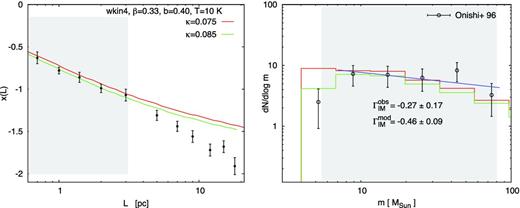
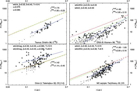
Structure and ClMF of the Taurus complex. Left: best fits x(L) of the data from LAL10 (dots with error bars) are plotted with lines, and their characteristics (equipartition relation, model parameter values) are specified. Right: ClMFs, derived from the same models (lines), are juxtaposed with the observational ClMF from molecular line maps (open symbols with error bars). The ranges of scales of clump generation (left) corresponding to the observational clump mass range, restricted by the lower limit of confidence of the model (right), are shown with shaded areas. A weighted power-law fit of the observational ClMF (blue line) is drawn. Its slope (obs) and the one of the modelled IM ClMF (mod) are specified.
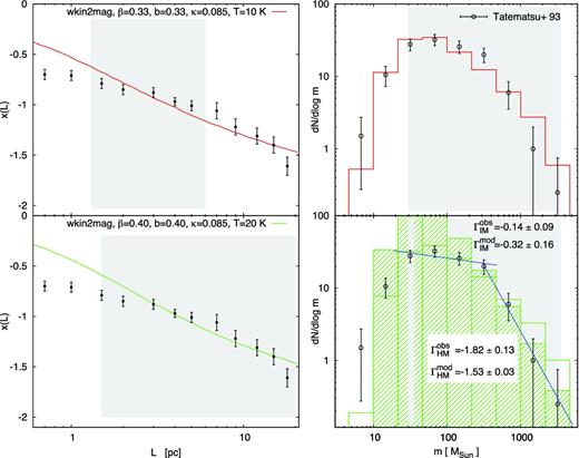
Structure and ClMF of the Orion A complex. The designations are the same as in Fig. 1; slopes of both IM and HM ClMF are specified. The modelled non-time-weighted (lines) and time-weighted ClMFs (hatched area) are shown. The completeness limit of the observational data is adopted as a lower mass limit of confidence.
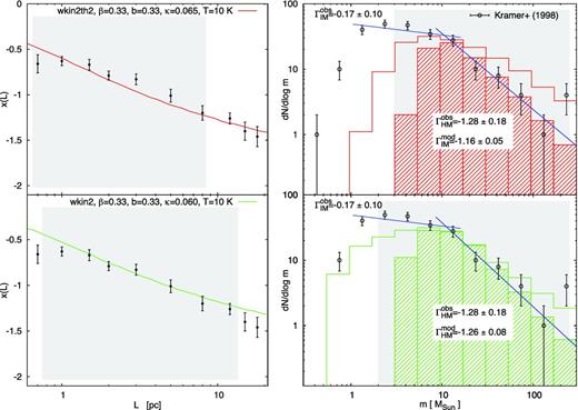
Structure and ClMF of the Orion B complex. The designations are the same as in Fig. 2.
Derivation of the ClMF
If only gravitationally unstable clumps are considered, one should take also into account their contraction in time-scales given by the free-fall time τff ∝ ρ−1/2. Their time-weighted mass function can be derived by permitting constant replenishment of the clump population and introducing a weighting factor of each scale of clump generation: |$w(L,x(L))\propto \tau _{\rm ff}^{-1}\propto \langle \rho \rangle ^{1/2}\propto L^{3x/2(1-x)}$| (cf. equations 2 and 11). Then the time-weighted ClMF obtained as the number of substructures |${\cal N}_L$| in equation (20) is modified by a factor w(L, x(L))/w(Lmax, x(Lmax)).
RESULTS
We put to test the ClMF, derived in Paper I, using molecular line observations of nearby Galactic MC complexes and dust continuum studies of further three regions at kpc-scale distances, mapped also in CO lines (Table 1). Subsamples of the original clump data are considered taking into account the lower mass limit of confidence in our models and/or the observational completeness limit; the corresponding size and mass ranges are specified in columns 3 and 4.
Observational clump samples used for comparison with the predictions of our model. Regions that are studied both by use of molecular line emissions and dust continuum data are shown in bold. The slope estimates are re-derived by us, adopting mass limits corresponding to the applicability of our model and to the data completeness range. Notation: D = approximate distance to the region, IM = intermediate-mass, HM = high-mass, γobs = slope [|$\text{d}\log m/\text{d}\log r$|] in the clump mass–size diagram, Mch = characteristic mass, CF = clump-finding (method), pHM = contour at half-maximum around intensity peaks, pPV = position–velocity diagrams passing through intensity peaks, GB = gravitationally bound, UB = unbound.
| SF region | D | Ref. | Sizes | Masses | γobs | Mch | ClMF slope | CF method | Note | |
|---|---|---|---|---|---|---|---|---|---|---|
| (kpc) | (pc) | (M⊙) | (M⊙) | IM | HM | |||||
| Molecular line studies | ||||||||||
| Taurus | 0.14 | 1 | |$0.07 -- 0.45$| | |$3--80$| | 1.95 | ≳100 | −0.27 | – | pHM | Mostly GB |
| Orion A | 0.45 | 2 | |$0.06 --0.35$| | |$30--1000$| | 1.14 | ∼300 | −0.14 | −1.82 | pPV | ∼90 per cent starless, GB? |
| Orion B | 0.45 | 3 | |$0.06 --0.70$| | |$3--200$| | 1.95 | ∼13 | −0.17 | −1.28 | gaussclumps | UB + GB |
| MC sample | ≤0.18 | 4 | |$0.08 --0.45$| | |$3--60$| | 2.09 | ∼10 | −0.25 | −1.45 | Various | Mainly starless, GB? |
| ≤0.18 | 4 | |$0.08--0.45$| | |$3--100$| | 2.09 | ∼13 | −0.44 | −1.77 | Various | Mainly starless, GB? | |
| M17 | 1.6 | 5 | |$0.03 --0.60$| | |$6--2300$| | 1.77 | ≳200 | −0.34 | −1.00 | gaussclumps | UB + GB? |
| Rosette | 1.6 | 6 | |$0.45 -- 4.5$| | |$30-- 2000$| | 2.40 | ≳800 | −0.28 | −1.13 | clumpfind | Starless, mostly UB? |
| Dust continuum studies | ||||||||||
| M17 | 1.6 | 7 | |$0.02 -- 0.70$| | |$1 -- 600$| | 2.13 | ∼100? | −0.35 | – | clumpfind | Mainly starless |
| M17 + NGC 7538 | 7, 8 | |$0.06 --0.60$| | |$3 --1000$| | 2.05 | ∼100 | −0.25 | −1.82 | clumpfind | UB + GB? | |
| Rosette | 1.6 | 9 | |$0.20 -- 0.70$| | |$1.7 -- 200$| | 2.22 | ≳9 | −0.57 | −1.04 | getsources | Starless |
Molecular line studies
Three individual nearby star-forming regions of comparable size are selected: (i) with clumps delineated through similar density tracers: 13CO (Orion B; Kramer et al. 1998), C18O (Taurus; Onishi et al. 1996) and CS (|$J=1--0$|) (Orion A; Tatematsu et al. 1993), consistent with the typical clump densities in our approach n ∼ 103–104 cm−3; (ii) with known general structure from dust extinction maps of LAL10. The spatial extent of the studied regions in the chosen complexes falls within the adopted inertial range of turbulence [Section 2.1, (i)]. Dust extinction data reveal some diversity of structure in terms of mass–size relation of regions delineated by isodensity contours: Taurus exhibits monotonically ‘steep’ structure in terms of x(L), while Orion A and Orion B have ‘shallow’ internal regions and ‘steep’ external, less dense regions (Figs 1–3, left-hand panels; cf. fig. 2 in LAL10). Taurus is a typical low-mass star-forming region (Kenyon, Gómez & Whitney 2008), while numerous HM stars have been formed in Orion A and B in the recent past. As an additional test of the predictive power of the models for a variety of environments, we perform comparisons with observational ClMF for a sample of nine MC complexes (Tachihara et al. 2002) wherein star-forming, cluster-forming and starless clumps have been detected.
An equipartition relation and a parameter set were sought that yield the best fit x(L) of the cloud structure as traced by the LAL10 data (Figs 1–3, left-hand panels). The modelled ClMF derived from them is compared with the observational one from molecular line maps (Figs 1–3, right-hand panels). The range of spatial scales considered in the fitting procedure (shaded areas, left-hand panels) corresponds to the mass range of the referred observational ClMF (shaded areas, right-hand panels), additionally restricted by the lower clump mass limit of confidence in the model. The scales are treated as those where the observed clumps were generated and hence their range is obtained through the clump mass-scale diagram of the tested model (Paper I, section 3.1).
Taurus
Fig. 1 (left) demonstrates that the equipartition choice wkin4 yields a very good fit of the inner parts of the complex. That seems physically consistent to us since this case describes structures which have been shaped under significant influence of self-gravity. The typical dense clumps generated in them have mass distributions in relatively good agreement with the observational ClMF (Fig. 1, right), obtained by Onishi et al. (1996). The best-fitting parameters point to a mainly solenoidal turbulent forcing (see Federrath, Klessen & Schmidt 2008) and a ‘soft’ velocity scaling, typical for incompressible turbulence. On the other hand, the equipartition relation wkin4 is obviously not applicable to the less dense extensive parts of the cloud. We stress, however, that in our model scales L > 3 pc do not produce clumps with masses within the considered observational range.
It should be pointed out that the ClMF obtained by Onishi et al. (1996) differs significantly from ClMFs in other clouds as derived from molecular line emission data. Using essentially the lowest mass bin (≃3 M⊙), these authors argue for a flat mass function1 in Taurus, although they remain open for an alternative interpretation based on an ‘unbiased survey… in a wide mass range’. We believe that indeed their data cover the mass range around the turn-over of the ClMF while its HM part (if existing) falls beyond their scope – note that characteristic masses Mch of hundreds of M⊙ are derived in various MC complexes (Table 1, column 7). The power-law slope of the modelled ClMF over the lower mass limit of confidence in our model is slightly shallower than the typical one of the mass distribution of CO clumps (Blitz 1993; Kramer et al. 1998). It would steepen (Γ ∼ −0.7) if the observational data contained clumps with masses up to the expected Mch ∼ 200 M⊙ – cf. the modelled ClMFs from wkin4 (fig. 3 in Paper I).
Orion A
We obtained good fits of the Orion A structure in the case wkin2mag at intermediate to large spatial scales (Fig. 2, left). The corresponding ClMFs generally agree with the result of Tatematsu et al. (1993). Enhancement of the model temperature, compatible with the derived T ∼ 20 K in the complex (Ikeda et al. 2007), leads to larger, more plausible values of b and β and yields a wider range of scales of clump generation as the cloud structure is better fitted through the curve x(L) (Fig. 2, bottom).
Depending on the model temperature, the case wkin2mag in our approach generates mostly/only gravitationally unstable clumps (Paper I, fig. 3). On the other hand, Tatematsu et al. (1993) claim that all clumps in their sample are close to virial equilibrium. Therefore, a time-weighted ClMF (cf. Section 2.3) is more appropriate for comparison with the referred observational study. Time weighting steepens the HM slope of the model from |$\Gamma {\rm ^{mod}_{HM}}\sim -1$|, typical for fractal clouds, to ∼−1.5, i.e. steeper than that of the stellar IMF (Γ ≃ −1.3; Salpeter 1955) (Fig. 2, bottom right). This leads to agreement (within the data uncertainties) with the observational ClMF for clump masses >Mch ∼ 300 M⊙, while for lower masses the deviation is drastic. In contrast, the non-weighted modelled ClMF is generally consistent with the observational ClMF below Mch and for T = 20 K. We note the high completeness limit (∼30 M⊙) of the data which might artificially constrain the IM range.
Orion B
The referred observational ClMF in this region is part of the work of Kramer et al. (1998), who analysed CO data sets for eight Galactic MCs. They argued for a single-power-law ClMF in all cases, with a universal mean slope Γ ∼ −0.7, over a wide range of clump masses. However, a closer look at their result for Orion B reveals that this MC may be an exception. The conclusion of Kramer et al. (1998) about a single power law with shallow slope is based mostly on the single mass bin ≳200 M⊙ (Fig. 3, right). Inspection of the statistically rich data in the range |$2--80$| M⊙ indicates rather a combination of two power laws: a shallow IM slope below 15 M⊙ and a significantly steeper HM slope. Adopting the latter value as Mch and the completeness data limit of the authors M ∼ 1 M⊙, one obtains |$\Gamma {\rm _{IM}^{obs}}$| similar to that in Orion A and a Salpeter-like |$\Gamma {\rm _{HM}^{obs}}$|.
Modelling of the Orion B structure as traced by the LAL10 data yields good fits in the cases wkin2th2 and wkin2 (Fig. 3, left). For such choices of equipartition and temperature T = 10 K, the critical mass over which most of the generated clumps are gravitational unstable is about the adopted characteristic mass from the used observational data. Therefore, we apply time weighting for the HM regime and obtain |$\Gamma {\rm _{HM}^{mod}}$| close to the Salpeter value. The modelled ClMFs fit remarkably well the HM observational ones, excluding the sole bin at the upper limit of the distribution (Fig. 3, right). Non-weighted ClMFs obviously fail to reproduce the observational one although the HM slope ∼−0.7 is close to the estimate of Kramer et al. (1998). The model is not applicable to fit the IM ClMF because of the high lower mass limit of confidence.
Sample of MC complexes
The presented best-fitting descriptions x(L) of MC structure in Taurus, Orion A and Orion B and their corresponding ClMFs with different characteristic masses Mch and HM slopes (cf. Table 1) are derived by use of different equipartition relations that may reflect a variety of physical conditions. What model case would describe appropriately a statistical ClMF obtained from a large set of clump data in different MCs? The sample in the study of Tachihara et al. (2002) could give a clue to the answer – it encompasses nearby cloud complexes of diverse star-forming type as the vast majority of clumps are associated with no or a small number young stellar objects and have masses below several dozens of M⊙. Clumps associated with young stellar clusters were found in two out of nine sampled clouds and their fraction is only 5 per cent of the total number of clumps. All objects with masses ≥115 M⊙ are from this group. One may take the latter value as an upper mass limit when fitting the ClMF, in order to avoid extreme environments and to secure sufficient statistics. The two-power-law shape of the ClMF is evident whereas the characteristic mass is ambiguous. We consider two choices which both allow for very good fits: (i) Mch ∼ 10 M⊙, adopting the estimate of Tachihara et al. (2002) and decreasing the upper mass limit further by one bin; and (ii) Mch ∼ 13 M⊙(Fig. 4). The lower mass limit in both cases is the lower limit of confidence of the tested models.
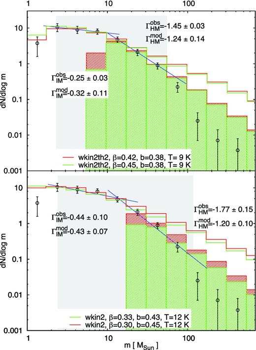
Modelling of the observational ClMF from nine Galactic star-forming regions by use of the equipartition relations wkin2 and wkin2th2 for κ = 0.065 and adopting characteristic mass ∼10 M⊙ (top) and ∼13 M⊙ (bottom). See the text for the considered mass ranges. Other designations are the same as in Figs 1–3.
Choice (i) yields excellent agreement of the model case wkin2th2 with the observational ClMF: time-weighted model for the HM part and non-time-weighted for the IM part (Fig. 4, top). The IM slope is very similar to the ones found in the considered individual MC complexes while the HM slope is about the Salpeter value, like in Orion B (Section 3.1.3). The discrepancy with the data for m ≳ 60 M⊙ could be attributed to incompleteness of the sample in this mass range. A Salpeter-like slope is to be expected for mass distributions of (nearly) virialized clumps assuming their formation at a constant rate. The effect will be similar if the ClMF is derived from a statistically significant sample containing clumps in complexes at different evolutionary stages of clump formation. Note also that the variation of the velocity scaling index β in the fitting models is consistent with most observational and numerical works (e.g. Padoan et al. 2006, 2009). The values of the b parameter indicate preliminary solenoidal turbulent forcing with small contributions of the compressive mode.
Considering choice (ii), an upper mass limit ∼115 M⊙ is adopted as mentioned above. The model case wkin2 provides an excellent fit of the IM ClMF and a problematic one – for the HM ClMF. Again, the completeness of the clump mass bin 60 ≤ m ≤ 100 M⊙ is an open issue which is crucial for the correct slope estimation. On the other hand, the obtained low velocity scaling index β is consistent with results for Taurus, Orion A and Orion B.
Modelling of the observational ClMF from the equipartition cases wkin2 and wkin2th2 suggests that most of the clumps generated in MC complexes of diverse star-forming activity and with mean density about the typical local density (cf. equation 7 in Paper I) are in a state close to virial equilibrium.
Clump mass–size diagrams
An additional test for adequacy of the proposed statistical modelling of the ClMF is to construct clump mass–size diagrams. The comparison between the used observational data and the best-fitting models of the observational ClMFs is displayed in Fig. 5. There are two difficulties with such an analysis. First, the ‘average clump ensembles’ in our model occupy narrow strips in |$m--r$| diagrams2, whereas the dispersion of the observational samples is huge. Secondly, mass and (especially) size determinations from molecular line maps depend essentially on the clump-finding technique which is different in each considered reference work (Table 1, column 10). A meaningful criterion is to compare the slope |$\gamma ^{\rm obs}=(\text{d}\log m/\text{d}\log r)$| in the observational |$m--r$| diagram with the predicted slopes γmod as the latter vary with the chosen equipartition case and the velocity scaling index β (cf. Paper I, fig. C1).
Clump mass–size diagrams from the referred molecular line studies. The data used to derive the ClMFs are shown with open symbols. The predictions of our model are plotted with dots, retaining the corresponding colours from Figs 1–4.
The predicted slopes from the best-fitting ClMF model are consistent with the ones from the referred molecular line studies within 1σ limit for Taurus and Orion A and within about 2σ limit for Orion B and for the sample of Tachihara et al. (2002). In two cases, the ‘average clump ensemble’ strips cross the region of the observational data (Fig. 5, bottom). Taking into account the good agreement between observational and modelled ClMFs (Figs 1–4), the shift between the two sets in the |$m--r$| diagrams – with a factor of 2 towards larger (Orion A) or smaller sizes, – is to be interpreted with the variety of the clump size definition. The issue will be commented further in the next section wherein we compare our model with ClMFs from dust continuum studies and in the discussion.
Dust continuum studies
Sensitive submillimetre continuum maps are appropriate for probing the MC structure on small scales due to the optically thin dust emission. In the last decade, the achieved angular resolutions of ≲20 arcsec from ground-based observations (e.g. SCUBA, Bolocam) and space missions like Herschel allowed for study of clumps with sizes ≳0.1 pc in complexes at distances over 1 kpc. Therefore, it is instructive to compare results from such studies with our model. In view of the complexes’ remoteness, the considered regions were not included in the work of LAL10 and we do not have at our disposal their dust extinction mapping as a tool to trace and fit the general cloud structure (cf. Figs 1–3, left). To compensate this lack, we chose star-forming regions whose clump population has been probed also by use of molecular line maps. The observational ClMF was fitted directly and the clump mass–size diagram was used as an additional test.
M17
Large part of this massive star-forming region was mapped by Reid & Wilson (2006a) in two SCUBA bands. We use here the clump data from their 850 μm map because of the richer statistics. The fitting of the observational ClMF and the corresponding clump mass–size diagram are plotted in Fig. 6 (top). A very good fit of the ClMF is achieved from the model case wkin4 that points to strongly gravitationally bound clumps. The predicted and the observational clump mass–size diagrams are also in agreement (Fig. 6, top right). Note that we assumed a higher gas temperature T = 20 K which is about the average clump temperature derived by the authors.
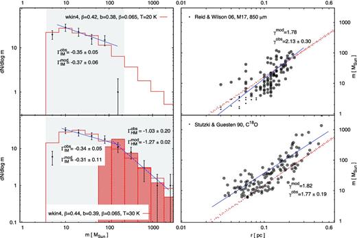
ClMF and clump mass–size diagrams of the star-forming region M17 from dust continuum (top) and molecular line (bottom) observations. The shaded areas denote the observational mass range restrained by the lower mass confidence limit from the model – the corresponding data used to derive the ClMFs are shown with open symbols in the m–r diagram. The predictions of the model are plotted with the same colours in the left (lines) and right (dots) panels.
Although Reid & Wilson (2006a) suggest a two-power-law ClMF with Mch ∼ 8 M⊙, it seems that their result hints rather at an order-of-magnitude higher characteristic mass. This is supported by the slope in the mass range 10 ≲ m ≲ 100 M⊙ which is similar to the IM slopes found from the referred molecular line studies (cf. Table 1). However, only two clumps with masses >100 M⊙ in the observational sample are far from sufficient for a plausible estimate of the characteristic mass. To clarify the issue, we apply our method to a C18O study of the south-western sector of M17 (Stutzki & Güsten 1990). As demonstrated in Fig. 6, bottom, the results for an IM ClMF with Mch ∼ 100 M⊙ are virtually the same, fitted from the same model case and free parameter values and slightly higher temperature. Moreover, the HM ClMF is also well fitted by the time-weighted mass distribution of gravitationally unstable clumps. Neglecting the mass bin >2000 M⊙, which contains only two clumps, the slope ΓHM is shallower than that of the stellar IMF.
For independent confirmation of this result, we composed a twice larger sample, including clump data from a similar study of NGC 7538 (Reid & Wilson 2005). As shown in Fig. 7, the ClMF is fitted again from the model case wkin4 and a similar parameter set (β, b) for a large range of clump masses 7 ≲ m ≲ 1000 M⊙, applying time weighting for the more massive clumps. In comparison to the mass distribution from the M17 sample, the IM slope shallows slightly and approaches the values from the molecular line studies of nearby MC complexes (cf. Table 1), while the HM slope is much steeper than that from Stuzki & Güsten's study and is identical with the one in Orion A (Fig. 2) although with a smaller Mch. The agreement of the model with the clump data in the |$m--r$| diagram is again excellent (Fig. 7, right).

Combined ClMF and clump mass–size diagram of the star-forming regions M17 and NGC 7538 from dust continuum observations. The designations are the same as in Fig. 6. The values of κ = 0.065 and T = 30 K are retained without change from the fitting of the M17 sample only.
Rosette MC
The abundant observational studies of this complex in the outer Galaxy indicated active star formation in the past and nowadays. Its clump population has been studied both on molecular line and dust continuum maps; we chose the works of Williams et al. (1995) and Di Francesco et al. (2010), respectively. The high-quality Herschel data used by the latter authors allow for derivation of the ClMF in a mass range spanning three orders of magnitude (Fig. 8, top left). Some incompleteness is sensible in the mass bins ≳10 M⊙ and has – in our view – two possible explanations. First, for the sake of our study we selected only starless clumps from the original sample. Secondly, Di Francesco et al. (2010) applied the getsources algorithm (Men’shchikov et al. 2012) for clump decomposition which favours identification of more compact (and less massive) objects.
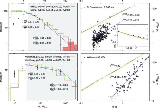
ClMF and clump mass–size diagrams of the Rosette MC from dust continuum (top) and molecular line (bottom) observations. The designations are the same as in Fig. 6. A comparison between the predictions of the illustrated models and the observed structure from a column density map using Herschel FIR continuum data (Schneider, private communication) is embedded in the top-right panel.
Because of the lower mass limit of confidence, our statistical method is not able to fit the ClMF below ∼2 M⊙. The observed mass distribution for larger masses could be interpreted as single-power-law ClMF with a slope of about −1 (not shown). In view of the possible incompleteness of the HM clump data, we suggest rather a two-power-law mass function, fitted from the model case wkin2 (Fig. 8, top left). The characteristic mass for wkin2 and for the obtained best-fitting parameters is ∼9 M⊙ (see fig. 3 in Paper I). Adopting this value for Mch, one gets a bit steeper IM ClMF than found for other MC complexes in this paper and an HM ClMF, with a slope typical for fractal clouds (Elmegreen 1997). In the clump mass–size diagram, a shift of the model from the observed clumps is evident like in some other studied regions: by a factor of 2–4 (Fig. 8, top right; cf. Fig. 5). Schneider (private communication) provided for us estimates of the cloud mass M as a function of the spatial scale L, calculated from the original Herschel column density map of Rosette. That enabled a check of the derived best-fitting model with the observed cloud structure, in terms of the LAL10 work (Figs 1–3, left). The shape of the modelled curve x(L) is consistent with the dust continuum data but with a shift towards lower x. Decreasing the mapping resolution parameter down to κ = 0.02, we found excellent agreement with the data (Fig. 8, right, embedded diagram). That is illustrative how the observed general cloud structure affects the κ-parameter space of the ClMF fitting.
Williams et al. (1995) derived the observational ClMF from CO mapping of Rosette MC. As seen in Fig. 8 (bottom), their clump size range practically does not overlap with the one of Di Francesco et al. (2010) while the mass range spans from 10 to >1000 M⊙. The ClMF is well fitted from the model case wkin2mag and a very ‘soft’ velocity scaling, β ≃ 0.20. Such values of the scaling index were found from MHD simulations of Collins et al. (2012).
DISCUSSION
The comparison with the considered molecular line and dust continuum studies of Galactic MC complexes demonstrates the applicability of a statistical approach to derive the ClMF presented in Paper I. The results on fitting the observational ClMF through our model are summarized in Table 2. They are obtained by use of two different primary fitting criteria: fitting of the general cloud structure x(L) − L or direct fitting of the ClMF. Regardless of the type of observational data, the applied fitting criterion and of the variety of model cases, the best-fitting parameters span relatively narrow ranges.
‘Soft’ velocity scaling: 0.20 ≲ β ≤ 0.46.
Mainly solenoidal forcing or a natural mixture of solenoidal and compressive modes: 0.30 ≤ b ≤ 0.46.
Mapping resolution from few per cent to one tenth of the spatial scale: 0.02 ≤ κ ≤ 0.10.
Typical temperatures for molecular gas phase: 8 ≤ T ≤ 35 K.
Summary of the results on fitting the observational ClMF in the considered MC complexes. The probed parameter ranges (footnote to the table) and the ranges of the model parameters that give good fits (columns 3–7) are specified. Notation: FC = fitting criterion (x − L – general cloud structure in the |$x(L)--L$| diagram; ClMF – direct fitting of the ClMF), MC = model case.
| SF region | FC | MC | Model parameter ranges | ClMF | |$m--r$| slope | |||||||
|---|---|---|---|---|---|---|---|---|---|---|---|---|
| β | b | κ | T (K) | |$\Gamma ^{\rm obs}_{\rm IM}$| | |$\Gamma ^{\rm mod}_{\rm IM}$| | |$\Gamma ^{\rm obs}_{\rm HM}$| | |$\Gamma ^{\rm mod}_{\rm HM}$| | γobs | γmod | |||
| Molecular line studies | ||||||||||||
| Taurus | x − L | wkin4 | 0.30–0.36 | 0.38–0.42 | 0.07–0.09 | 10–20 | |$-0.27{\small \pm 0.17}$| | |$-0.46{\small \pm 0.09}$| | – | – | |$1.95{\small \pm 0.23}$| | 1.75 |
| Orion A | x − L | wkin2mag | 0.38–0.42 | 0.38–0.42 | 0.07–0.09 | 18–22 | |$-0.14{\small \pm 0.09}$| | |$-0.32{\small \pm 0.16}$| | |$-1.82{\small \pm 0.13}$| | |$-1.53{\small \pm 0.03}$| | |$1.14{\small \pm 0.40}$| | 1.42 |
| Orion B | x − L | wkin2 | 0.30–0.36 | 0.30–0.36 | 0.055–0.065 | 10–15 | |$-0.17{\small \pm 0.10}$| | – | |$-1.28{\small \pm 0.18}$| | |$-1.26{\small \pm 0.08}$| | |$1.95{\small \pm 0.15}$| | 1.62 |
| x − L | wkin2th2 | 0.30–0.36 | 0.30–0.36 | 0.050–0.065 | 10–15 | |$-0.17{\small \pm 0.10}$| | – | |$-1.28{\small \pm 0.18}$| | |$-1.16{\small \pm 0.05}$| | |$1.95{\small \pm 0.15}$| | 1.60 | |
| MC sample | ClMF | wkin2 | 0.30–0.36 | 0.42–0.46 | 0.02–0.10 | 10–12 | |$-0.44{\small \pm 0.10}$| | |$-0.43{\small \pm 0.07}$| | |$-1.77{\small \pm 0.15}$| | |$-1.20{\small \pm 0.10}$| | |$2.09{\small \pm 0.16}$| | 1.60 |
| ClMF | wkin2th2 | 0.42–0.46 | 0.36–0.40 | 0.02–0.10 | 8–10 | |$-0.25{\small \pm 0.03}$| | |$-0.32{\small \pm 0.11}$| | |$-1.45{\small \pm 0.03}$| | |$-1.24{\small \pm 0.14}$| | |$2.09{\small \pm 0.16}$| | 1.65 | |
| M17 | ClMF | wkin4 | 0.43–0.45 | 0.37–0.40 | 0.02–0.10 | 28–35 | |$-0.34{\small \pm 0.05}$| | |$-0.31{\small \pm 0.11}$| | |$-1.03{\small \pm 0.20}$| | |$-1.27{\small \pm 0.02}$| | |$1.77{\small \pm 0.19}$| | 1.82 |
| Rosette | ClMF | wkin2mag | 0.18–0.23 | 0.30–0.36 | 0.02–0.10 | 8–15 | |$-0.28{\small \pm 0.03}$| | |$-0.26{\small \pm 0.09}$| | |$-1.13{\small \pm 0.24}$| | |$-1.06{\small \pm 0.10}$| | |$2.40{\small \pm 0.17}$| | 1.30 |
| Dust continuum studies | ||||||||||||
| M17 | ClMF | wkin4 | 0.40–0.44 | 0.37–0.40 | 0.02–0.10 | 28–35 | |$-0.35{\small \pm 0.05}$| | |$-0.37{ \small \pm 0.06}$| | – | – | |$2.13{\small \pm 0.30}$| | 1.78 |
| M17+ | ClMF | wkin4 | 0.43–0.46 | 0.38–0.42 | 0.02–0.10 | 28–35 | |$-0.25{\small \pm 0.04}$| | |$-0.33{ \small \pm 0.10}$| | |$-1.82{\small \pm 0.11}$| | |$-1.25{\small \pm 0.09}$| | |$2.05{\small \pm 0.08}$| | 1.89 |
| Rosette | ClMF | wkin2 | 0.44–0.46 | 0.41–0.45 | 0.02–0.03 | 18–25 | |$-0.57{\small \pm 0.13}$| | |$-0.56{\small \pm 0.07}$| | |$-1.04{\small \pm 0.33}$| | |$-0.93{\small \pm 0.02}$| | |$2.22{\small \pm 0.25}$| | 1.86 |
| (x − L ) | ||||||||||||
Probed parameter spaces: 0.18 ≤ β ≤ 0.65; 0.30 ≤ b ≤ 0.55; 0.02 ≤ κ ≤ 0.10; 8 ≤ T ≤ 40 K.
A small velocity scaling index β, close or equal to the Kolmogorov value for incompressible turbulence (0.33), may seem unrealistic in view of the high compressibility of interstellar turbulence which implies β ∼ 0.50. In fact, numerical simulations of magnetized clouds show that the velocity power spectrum can be even shallower than in the Kolmogorov theory. Collins et al. (2012) measured |$\beta =0.23--0.29$| for the thermal-to-magnetic pressure ratio in range |$0.2--2.0$|. [In our modelling, the latter value could be as low as ≃0.05 in the case wkin2mag; see equation (3).] Apparently, the velocity scaling index for incompressible turbulence β = 0.33 should not be necessarily treated as the lowest possible value from theoretical considerations.
The best-fitting range of the turbulent forcing parameter b is narrower, with typical values |$0.38--0.40$|, in most considered complexes. Since b can vary within a star-forming region, this result might be explained as a statistical effect. Indeed, b ≃ 0.40 corresponds to a natural mixture of solenoidal and compressive modes as the latter represent longitudinal waves, occupying one of the three spatial dimensions (see Federrath et al. 2010, and fig. 8 there). The typical best-fitting values of the mapping resolution parameter κ are about several per cent. These are the expected values, appropriate to distinguish substructures which are significantly smaller than the spatial scale L and significantly larger than the scale of dissipation.
Generally, our results lend support to a two-power-law shape of the ClMF: IM and HM part, with two distinct values of the characteristic mass Mch: ∼10 and ∼200 M⊙. (The molecular line study of Rosette MC with its high Mch is the only exception.) The first value is consistent with model cases of a ‘virial-like’ equipartition between gravitational and turbulent energy, possibly with contribution of the thermal energy at small scales and negligible contribution of the magnetic energy (wkin2, wkin2th2). These equipartition relations are not sufficient to argue that the modelled clumps are in virial equilibrium (Ballesteros-Paredes 2006) but rather indicate their gravitational boundedness or contraction. On the other hand, if the considered model cases hold for a whole cloud, they are indicative for its global collapse (Vázquez-Semadeni et al. 2007). Large characteristic masses of hundreds of M⊙ are obtained for strongly gravitating clumps, with possible magnetic support (wkin4, wkin2mag). Such are evidently the cases in Taurus, Orion A, M17 and NGC 7538.
The slope of the modelled IM ClMF is shallow and does not vary significantly from complex to complex (|$-0.26\ge \Gamma _{\rm IM}^{\rm mod}\ge -0.56$|) while the variety is larger for the HM one: from typical slopes for fractal clouds to slopes, a bit steeper than the one of the stellar IMF (|$-0.9\gtrsim \Gamma _{\rm HM}^{\rm mod}\gtrsim -1.5$|). It seems that the single-power-law observational ClMFs of slope −0.7 ≳ Γobs ≳ −0.8 derived from molecular line studies in 1990s (Stutzki & Güsten 1990; Blitz 1993; Heithausen et al. 1998) have been products of a combination of IM ClMF and a few bins from HM ClMF. On the other hand, the variety of HM ClMF slopes probably reflects a real variety of physical conditions in individual complexes and the gravitational balance and evolution of the dense fragments in them. Its model slope |$\Gamma ^{\rm mod}_{\rm HM}$| is similar to that of the stellar IMF when the ClMF is time weighted. When derived from molecular line mapping of Orion A (Tatematsu et al. 1993) or the dust continuum studies of M17 and NGC 7538 by Reid & Wilson (2005, 2006a), |$\Gamma ^{\rm obs}_{\rm HM}$| exceeds noticeably the Salpeter value but lies still within the observed variability range (Kroupa 2001).
The dust extinction mapping of Taurus, Orion A and Orion B by LAL10 enabled us to make a link between the predicted general cloud structure and the ClMF. We point out also the excellent agreement applying this criterion to the dust continuum study of Rosette, making use of a column density map of Rosette (Fig. 8, top right, embedded) obtained from Herschel data (see Schneider et al. 2012 for details). (Note that the extinction map derived from near-IR extinction using 2MASS (Schneider et al. 2011) delivers similar values for AV ≲ 10m.) Generally, good agreement is found for the chosen scales of clump generation L between ∼0.5 and ∼15 pc while in Taurus the upper limit is about half of that. Those are the conservative limits of the inertial range of turbulence3 that is a corner stone in our framework of clump description. The discrepancies for larger L are to be expected and can be interpreted as reflecting changes in the physical conditions – such scales may lie outside the inertial range and/or the assumption of isothermality does not hold for them (e.g. Hennebelle et al. 2008). On the other hand, at L ≲ 1 pc the density pdf deviates from the lognormal shape and develops a power-law tail in the high-density part (Klessen 2000; Kritsuk, Norman & Wagner 2011; Federrath & Klessen 2013). The predicted typical clump size in such density regimes approaches ∼0.1 pc which is about the sonic scale for the temperature range 10–20 K, i.e. the assumption for supersonic turbulence as a generator of clumps breaks down.
Inclusion of data from dust continuum studies in the analysis of the clump mass–size (|$m--r$|) diagrams confirms the results from molecular line mappings (Section 3.1.5): consistency between the slopes within 2σ and, occasionally, a shift by a factor of up to 3 on the size axis. Generally, the agreement between the locations of the ‘average clump ensemble’ and the observed clumps is better, especially, for the combined clump sample from M17 and NGC 7538. The discrepancies in the |$m--r$| diagrams could be attributed to the various clump-finding techniques used in the referred observational studies (cf. Table 1, column 10) and hence to different clump size definitions. The latter would not lead to substantially different mass estimates if a typical clump structure is a dense central region and diffuse outer shell. A careful comparative analysis of the basic clump-finding algorithms, applied to identical observational or numerical data sets, is necessary for a more comparison between our statistical clump description and the observed clumps in MC complexes.
The role of the magnetic fields in shaping the physical characteristics of MCs and of their substructures can be accounted for more thoroughly in a further extension of this work. Molina et al. (2012) proposed an analytical model of the relation between the width of the pdf σ in magnetized turbulent medium. It includes a modification of equation (5), consistent with a scaling law of magnetic field B ∝ 〈ρ〉1/2 (equation 3) and can be easily incorporated in our modelling.
Finally, we caution the reader that the predictions of our model hold for less evolved clumps of sizes |$\gtrsim 0.1--0.2$| pc and must not be compared with observational mass distributions of dense (prestellar) cores. The latter ones will be subject of another study which considers the high-density power-law tail of the density pdf (cf. Kainulainen et al. 2009; Kritsuk et al. 2011) in active star-forming regions as a basis for cores’ description. The essence of this approach is presented in Donkov, Stanchev & Veltchev (2012) while the model is in process of development. Such study may answer the question of whether the difference between the ClMF and the CMF is physical or statistical.
SUMMARY
Our statistical approach for physical description of condensations (clumps) formed through a turbulent cascade during the early MC evolution predicts: (i) the cloud structure in terms of effective size–mass scaling relations, through the mass–density exponent x as a function of the spatial scale L (DVK11); and (ii) the composite ClMF (Paper I). Different models within this framework are generated by choosing an appropriate energy equipartition relation and a set of four free parameters: velocity scaling index β, turbulent forcing parameter b, mapping resolution parameter κ and temperature T. In this paper, we compared ClMFs from molecular line and dust continuum studies of Galactic cloud complexes with ones derived from our model applying alternative fitting criteria: fitting the structure x(L) of individual complexes (when additional dust extinction data are available) or direct fitting of the observational ClMF.
Both fitting criteria lead to modelled clump mass distributions, in good or excellent agreement with the considered observational data. The equipartition relations which yield these fits indicate gravitational boundedness of the dominant clump population in the considered clouds, possibly including the contribution of magnetic or thermal energy: model cases wkin2, wkin2th2 or wkin2mag. On the other hand, the results for Taurus, M17 and NGC 7538 rather hint at strongly gravitating or contracting inner parts of those complexes (model case wkin4). The derived best-fitting values of the parameters β, b and T for all studied individual clouds span relatively narrow ranges. In most MC complexes, the typical velocity scaling index is found to be similar to the original ‘Larson's first law’ (equation 1, β = 0.38) or to β ∼ 0.43 testified from recent observations (Padoan et al. 2006, 2009). The best-fitting values of the turbulent forcing parameter concentrate around b ≃ 0.40 which corresponds to a natural mixture of compressive and solenoidal modes (Federrath et al. 2010).
The modelled clump mass distributions support a ClMF which might be represented as a combination of two-power-law functions. The latter are separated by a characteristic mass Mch that varies typically within one order of magnitude or more: from about ten to hundreds of solar masses. The slope of the IM ClMF is shallow and nearly constant: −0.25 ≳ ΓIM ≳ −0.55. The HM part of the ClMF corresponds to gravitationally unstable clumps in all considered model cases, and hence a more appropriate description should take into account the dynamical clump evolution. Such a description is achieved through time weighting of the clump mass distribution. (The effect will be similar if the ClMF is derived from a statistically significant sample containing clumps in MC complexes at different evolutionary stages of clump formation.) We obtained slopes within a broader range −0.9 ≳ ΓHM ≳ −1.6 that includes the typical value for fractal clouds −1 (Elmegreen 1997) as well that of the stellar IMF (Salpeter 1955).
A comparison between the observational and the modelled clump mass–size diagrams reveals agreement of the slopes within the 2σ limit and, in most cases, a systematic shift towards smaller or larger clump sizes. The latter is to be attributed to variety of size definitions used in the different clump-finding techniques.
We are grateful to the anonymous referee for his/her insightful comments and recommendations which helped us to improve substantially this paper. We thank J. Di Francesco for the list of clump properties in Rosette MC derived from Herschel data and N. Schneider for providing us the mass/spatial scale values shown in Fig. 8 from the same Herschel column density map. We appreciate the help of V. Ossenkopf and R. Simon who provided for us data on the individual clump characteristics in Orion B from the original study of Kramer et al. (1998).
TV acknowledges support by the Deutsche Forschungsgemeinschaft (DFG) under grant KL 1358/15-1.
A shallow mass spectrum, in their terms.
Clump sizes from our model are converted to radii r = l/2 to be compared with the radii of observed clumps.
We recall here comment (i) in Section 2.1.
