


Abstract
We aim at characterizing dense cores in the clustered environments associated with intermediate-/high-mass star-forming regions. For this, we present a uniform analysis of Very Large Array NH3 (1,1) and (2,2) observations towards a sample of 15 intermediate-/high-mass star-forming regions, where we identify a total of 73 cores, classify them as protostellar, quiescent starless, or perturbed starless, and derive some physical properties. The average sizes and ammonia column densities of the total sample are ∼0.06 pc and ∼1015 cm−2, respectively, with no significant differences between the starless and protostellar cores, while the linewidth and rotational temperature of quiescent starless cores are smaller, ∼1.0 km s−1 and 16 K, than linewidths and temperatures of protostellar (∼1.8 km s−1 and 21 K), and perturbed starless (∼1.4 km s−1 and 19 K) cores. Such linewidths and temperatures for these quiescent starless cores in the surroundings of intermediate-/high-mass stars are still significantly larger than the typical linewidths and rotational temperatures measured in starless cores of low-mass star-forming regions, implying an important non-thermal component. We confirm at high angular resolutions (spatial scales ∼0.05 pc) the correlations previously found with single-dish telescopes (spatial scales ≳ 0.1 pc) between the linewidth and the rotational temperature of the cores, as well as between the rotational temperature and the linewidth with respect to the bolometric luminosity. In addition, we find a correlation between the temperature of each core and the incident flux from the most massive star in the cluster, suggesting that the large temperatures measured in the starless cores of our sample could be due to heating from the nearby massive star. A simple virial equilibrium analysis seems to suggest a scenario of a self-similar, self-gravitating, turbulent, virialized hierarchy of structures from clumps (∼0.1–10 pc) to cores (∼0.05 pc). A closer inspection of the dynamical state taking into account external pressure effects reveals that relatively strong magnetic field support may be needed to stabilize the cores, or that they are unstable and thus on the verge of collapse.
INTRODUCTION
The initial conditions of the star formation process in clusters are still poorly understood. Studies have unveiled the physical and chemical properties of starless isolated low-mass cores on the verge of gravitational collapse in nearby low-mass star-forming regions, showing that they have dense (n ∼ 105–106 cm−3) and cold (T ∼ 10 K) nuclei (e.g. Tafalla et al. 2002, 2004; Schnee et al. 2010), and that the internal motions are thermally dominated, as demonstrated by their close-to-thermal linewidths, even when observed at low angular resolution (see Bergin & Tafalla 2007, for a review). In the cold and dense nuclei of these cores, C-bearing molecular species such as CO and CS are strongly depleted (e.g. Caselli et al. 2002; Tafalla et al. 2002), while N-bearing species such as N2H+ and NH3 maintain large abundances in the gas phase (e.g. Caselli et al. 2002; Crapsi et al. 2005).
One major issue that has so far been poorly investigated is if, and how, the environment influences the physical and chemical properties of these pre-stellar cores. In clusters containing several forming stars in a small volume (of diameter ≤0.1 pc), turbulence, relative motions and interaction with nearby forming (proto-)stars can affect the less evolved condensations (e.g. Ward-Thompson, André & Crutcher 2007). Such an interaction is expected to be much more important in clusters containing intermediate-/high-mass protostars or newly formed massive stars, given the typical energetic feedback associated with the earliest stages of massive star formation (powerful outflows, strong winds, expanding H ii regions) and the high pressure of the parental pc-scale clumps. There is also vigorous theoretical debate on how star formation proceeds in clustered regions. Specifically: are the local kinematics of the gas dominated by feedback from protostellar outflows of already-forming, generally low-mass stars or from feedback from high-mass stars (Nakamura & Li 2007)? Can a model of star formation starting from quiescent starless cores, which has been successfully developed to explain observations of regions of isolated low-mass star formation, be applied to clustered regions (McKee & Tan 2003)? To constrain theoretical models, it is crucial to measure the main physical and chemical properties of starless and star-forming cores in clustered environments.
An observational effort in this direction has started, but it is mostly concentrated on nearby low-mass star-forming regions like Ophiuchus (e.g. André et al. 2007; Friesen et al. 2009) and Perseus (e.g. Foster et al. 2009), due to the fact that the typical large distances (≥1 kpc) of high-mass star-forming regions make the study of clustered environments very challenging. Foster et al. (2009) and Friesen et al. (2009) show that starless cores (studied at spatial scales ∼0.01–0.05 pc) within low-mass star-forming clusters have typically higher kinetic temperatures (∼13–14 K) than low-mass isolated cores (∼10 K). On the other hand, the kinematics of these low-mass protoclusters seem to be dominated by thermal motions like in more isolated cores, even though the external environment is turbulent (André et al. 2007). On the contrary, in the very few published studies of (proto-)clusters containing an intermediate-/high-mass forming star, the internal motions of starless cores are dominated by turbulence (see e.g. Fontani et al. 2008, 2009 for IRAS 05345+3157; Wang et al. 2008 for G28.34+0.06; Pillai et al. 2011 for G29.96−0.02 and G35.20−1.74; Fontani et al. 2012b for IRAS 20343+4129).
By using ammonia, Palau et al. (2007b) measured the temperature of the starless cores in the high-mass proto-cluster IRAS 20293+3952 at spatial scales of ∼0.05 pc, through Very Large Array (VLA) observations of the NH3 (1,1) and (2,2) inversion transitions. In fact, NH3 is the ideal thermometer for cold and dense gas because it is produced by the volatile molecular nitrogen, which is not expected to freeze out even in very cold and dense gas, and the NH3 (2,2) to (1,1) line ratio is sensitive to temperature (e.g. Ho & Townes 1983). Moreover, because other volatile species (like N2H+) cannot be used to derive the temperature, ammonia is the unique tracer for this purpose. Palau et al. (2007b) found temperatures of 16 K for starless cores in IRAS 20293+3952, i.e. higher than those measured in isolated low-mass starless cores (or infrared dark clouds with no active star formation; e.g. Ragan, Bergin & Wilner 2011), but similar to the values measured in active clustered cores in Perseus and Ophiuchus.
In this paper, we study a sample of 15 massive star-forming regions (see Table 1) observed with the VLA (providing an average spatial resolution of ∼0.05 pc) and analysed them in a uniform way. The main goal is to understand whether the results obtained in the few examples shown above are also obtained when analysing a statistically significant sample. The regions were selected according to the following criteria: (i) regions must be at distances ≲ 3.5 kpc, to obtain spatial resolution ≲ 0.05 pc, similar to the scale of the cores (0.03–0.2 pc: e.g. Bergin & Tafalla 2007); (ii) regions must have bolometric luminosities larger than ∼300 L⊙, which are the luminosities where clustering seems to be important (e.g. Testi, Palla & Natta 1999; Palau et al. 2013) and (iii) regions must be still associated with important amounts of gas and dust judging from single-dish observations of dust and molecular gas studies (e.g. Molinari et al. 1996; Beuther et al. 2002a; Mueller et al. 2002).
OBSERVATIONS
The VLA1 was used to observe the ammonia (J, K) = (1,1) and (2,2) inversion transitions towards 15 intermediate-/high-mass star-forming regions. These observations are part of different observational projects carried out on different epochs (from 1999 to 2009), and with the array in compact configurations (C, DnC or D). In Table 1 we list the 15 massive star-forming regions, indicating the name of the VLA project and the coordinates of the phase centre for each region. More technical details of each observational project, such as calibrators and epochs, are provided in Table 2. The full-width at half-maximum of the primary beam at the frequency of the observations (∼23.7 GHz) is approximately 2 arcmin. The spectral setup configuration used in each project (i.e. bandwidth and spectral resolution) is indicated in Table 2. The absolute flux scale was set by observing the quasars 1331+305 (3C286), 0137+331 (3C48) or 0319+415 (3C84), for which we adopted a flux of 2.41 Jy, 1.05 Jy and 16 Jy, respectively. Gain calibration was done against nearby quasars, which were typically observed at regular time intervals of ∼5–10 min before and after each target observation. Flux calibration errors could be up to 20–30 per cent. The data reduction followed the VLA standard guidelines for calibration of high-frequency data, using the National Radio Astronomy Observatory package aips. Final images were produced with the task imagr of aips, with the robust parameter of Briggs (1995) typically set to 5, corresponding to natural weighting. Two sources (AFGL 5142 and 22198+6336) were observed in different projects with different angular resolutions. For these sources we combined the uv-data to improve the sensitivity and uv-coverage of the final images. The resulting synthesized beams and rms noise levels (per channel) are indicated in Table 1.
Massive star-forming regions observed in NH3 with the Very Large Array, and a few observational and derived parameters.
| d | Lbol | VLA | Phase centreb | Synthesised beamc | CLUMPFINDe | |||||||
|---|---|---|---|---|---|---|---|---|---|---|---|---|
| Regiona | (kpc) | (L⊙) | project | RA | Dec. | HPBW | PA | RMSd | P | B | S | |
| 1. 00117+6412 | 1.8 | 1300 | AB1217 | 00:14:27.725 | +64:28:46.17 | 3.9 × 3.5 | +46 | 2.2 | 66 | 35 | 10 | |
| 2. AFGL5142 | 1.8 | 2200 | AZ120f | 05:30:48.024 | +33:47:54.44 | 3.6 × 2.6 | −14 | 3.5 | 203 | 20 | 10 | |
| 3. 05345+3157NE | 1.8 | 630 | AF471 | 05:37:52.400 | +32:00:06.00 | 2.3 × 2.3 | +92 | 1.4 | 39 | 25 | 5 | |
| 4. 05358+3543NE | 1.8 | 3100 | AC733 | 05:39:12.600 | +35:45:52.30 | 5.8 × 4.1 | +53 | 5.3 | 269 | 40 | 10 | |
| 5. 05373+2349 | 1.6 | 1100 | AF484 | 05:40:24.500 | +23:50:55.00 | 3.1 × 2.2 | −73 | 4.0 | 116 | 30 | 10 | |
| 6. 19035+0641 | 2.2 | 7700 | AF386 | 19:06:01.610 | +06:46:35.80 | 4.0 × 3.7 | −13 | 2.6 | 378 | 28 | 10 | |
| 7. 20081+3122 | 2.5 | 28 200 | AF386 | 20:10:09.050 | +31:31:35.20 | 5.0 × 4.4 | −56 | 3.3 | 602 | 25 | 5 | |
| 8. 20126+4104 | 1.64 | 8900 | AZ113 | 20:14:26.053 | +41:13:31.49 | 3.6 × 3.2 | +10 | 3.8 | 873 | 20 | 10 | |
| 9. G75.78+0.34 | 3.8 | 96 000 | AF386 | 20:21:43.970 | +37:26:38.10 | 3.7 × 3.4 | −57 | 3.8 | 181 | 30 | 5 | |
| 10. 20293+3952 | 2.0 | 8000 | AZ120 | 20:31:10.698 | +40:03:10.75 | 6.9 × 3.1 | +72 | 3.0 | 240 | 40 | 10 | |
| 11. 20343+4129 | 1.4 | 1500 | AS708 | 20:36:07.301 | +41:39:57.20 | 4.2 × 3.2 | +11 | 3.5 | 224 | 27 | 10 | |
| 12. 22134+5834 | 2.6 | 11 800 | AK558 | 22:15:08.099 | +58:49:10.00 | 3.8 × 3.1 | +88 | 1.5 | 31 | 40 | 10 | |
| 13. 22172+5549N | 2.4 | 830 | AF484 | 22:19:08.600 | +56:05:02.00 | 3.2 × 3.0 | +17 | 1.2 | 61 | 30 | 10 | |
| 14. 22198+6336 | 0.76 | 340 | AS926f | 22:21:26.764 | +63:51:37.89 | 3.7 × 3.1 | −41 | 3.8 | 61 | 40 | 10 | |
| 15. CepA | 0.7 | 25 000 | AF386 | 22:56:17.870 | +62:01:48.60 | 5.4 × 4.9 | −29 | 3.6 | 332 | 30 | 6 | |
aName of regions starting with numbers (e.g. 00117+6412) refers to the IRAS name (Neugebauer et al. 1984).
bPhase centre coordinates (in Equatorial J2000.0) of the ammonia maps. Right ascension in units h:m:s and declination in units d:m:s.
cSynthesized beam [half-power beam width (HPBW)] in arcsec and position angle (PA) in degrees.
dRMS noise level, in units of mJy beam−1, per channel (of 0.3 km s−1 or 0.6 km s−1; see Table 2).
eP: intensity peak (in mJy km s−1) of the zero-order moment map. B (bottom) and S (step) parameters, in percentage of the peak, used in the CLUMPFIND algorithm to extract the position of the cores (see Section 3.1).
fAFGL5142 and 22198+6336 include also data of the project AZ114.
Configurations used, epochs, calibrators and spectral setup of the Very Large Array observational projects.
| VLA | Epoch | Flux | Gain calibrators | Bandwidth | Spectral resolution | ||||
|---|---|---|---|---|---|---|---|---|---|
| Project | config. | of observation | calibrator | (bootstrapped fluxes, Jy) | (MHz) | (kHz) | (km s−1) | ||
| AB1217 | D | 2007 | May | 3C286,3C48 | J0102+584 | 3.85 ± 0.06 | 3.125 | 48.8 | 0.6 |
| AC733 | DnC | 2004 | Jun | 3C84 | J0530+135 | 3.33 ± 0.02 | 3.125 | 48.8 | 0.6 |
| AF386 | D | 2001 | Jan | 3C286 | J2025+337 | 2.50 ± 0.04 | 3.125 | 48.8 | 0.6 |
| J1849+005 | 0.81 ± 0.01 | ||||||||
| J2322+509 | 0.72 ± 0.01 | ||||||||
| AF471 | D | 2009 | Oct/Nov | 3C286,3C48 | J0555+398 | 3.15 ± 0.01 | 3.125 | 24.4 | 0.3 |
| AF484 | D | 2009 | Oct/Nov | 3C48 | J0559+238 | 0.80 ± 0.01 | 3.125 | 24.4 | 0.3 |
| J2148+611 | 0.63 ± 0.01 | ||||||||
| AK558 | D | 2003 | May | 3C286 | J2148+611 | 0.60 ± 0.01 | 3.125 | 48.8 | 0.6 |
| AS708 | C | 2001 | Jul | 3C286 | J2015+371 | 2.34 ± 0.04 | 3.125 | 48.8 | 0.6 |
| AS926 | C | 2008 | Apr | 3C286,3C48 | J2146+611 | 0.72 ± 0.02 | 3.125 | 48.8 | 0.6 |
| AZ113 | D | 1999 | May | 3C286,3C48 | J2013+370 | 2.27 ± 0.21 | 3.125 | 24.4 | 0.3 |
| AZ114 | D | 1999 | Mar | 3C48 | J2230+697 | 0.43 ± 0.01 | 3.125 | 48.8 | 0.6 |
| J0552+398 | 3.46 ± 0.05 | ||||||||
| AZ120 | C | 2000 | Apr | 3C48 | J0552+398 | 4.72 ± 0.15 | 3.125 | 48.8 | 0.6 |
| D | 2000 | Sept | 3C48 | J0552+398 | 3.38 ± 0.04 | ||||
| J2015+371 | 3.84 ± 0.02 | ||||||||
RESULTS AND ANALYSIS
Core identification and classification
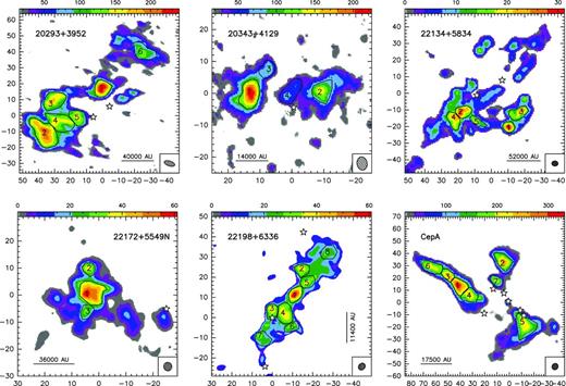
In Fig. 1, we present the zero-order moment (velocity-integrated intensity) maps of the NH3 (1,1) emission for the 15 massive star-forming regions studied in this work, while in Fig. B1, we present the first-order (intensity-weighted mean vLSR) and second-order (intensity-weighted mean velocity linewidth) moment maps. The zero-order moment maps were constructed by integrating the emission of all the hyperfine components, while for the first- and second-order moment maps we considered only the main hyperfine component, except for 20126+4104 for which the inner satellite hyperfine component was used (in the zeroth, first- and second-order moments) to avoid the high opacities in the main line. The integrated intensity maps reveal ammonia emission in all the regions, coming from compact condensations surrounded by faint and more extended emission. In the first-order moment maps (see Fig. B1), we identify large-scale velocity gradients (see e.g. AFGL 5142, 20081+3122, G75.78+0.34, 22172+5549N), not only associated with the compact condensations or cores but also with the whole ammonia emission, probably revealing the large-scale kinematics of the cloud. To extract and identify the cores within each region we ran the two-dimensional CLUMPFIND algorithm (Williams, de Geus & Blitz 1994) on the NH3 (1,1) zero-order moment map. This algorithm requires two input parameters: the ‘bottom’ level, corresponding to the lowest intensity to be included in the core, and the ‘step’, which determines the intensity increment required to differentiate one core from another core (see e.g. Miettinen et al. 2012 for further details). In our case, we used ‘bottom’ values of around 20–40 per cent of the peak intensity of the zero-order moment, and ‘steps’ in the range 5–10 per cent of the peak intensity (see last columns in Table 1). The output parameters defining each core returned by CLUMPFIND are the peak position, peak intensity and the flux density of the core. For each identified core we defined a polygon at the level of the full width at half-maximum (FWHM; see black thick lines in Fig. 1). In Table 3 we list the offset position of each core (relative to the phase centre; listed in Table 1) and the deconvolved FWHM size. A total of 73 cores were identified.
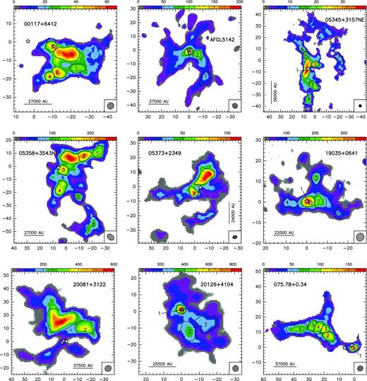
Colour image: NH3 (1,1) zero-order moment (integrated intensity) maps in units of mJy km s−1 (horizontal colour bar on the top of each panel). Coordinates in the x- and y-axis are right ascension and declination offsets in arcsec, with the (0,0) corresponding to the phase centre of the map (see Table 1). Black thick lines show the polygons for each core listed in Table 3, as obtained from the CLUMPFIND analysis (see Section 3). The numbers inside the polygons identify the core (see Table 3). The synthesized beams (listed in Table 1) are shown in the bottom-right corner of each panel. Star symbols in all panels correspond to centimetre continuum sources.
– continued
Physical parameters of the ammonia cores identified towards the 15 massive star-forming regions.
| Offseta | Sizeb | NH3 (1,1)c | NH3 (2,2)c | |||||||||||
|---|---|---|---|---|---|---|---|---|---|---|---|---|---|---|
| ID Region | No. | Δx | Δy | (pc) | A × τ | v | Δv | τd | Tmb | v | Δv | Trote | |$N_\mathrm{NH_\mathrm{3}}$|e | |
| 01 00117+6412 | 1 | −20.5 | −7.0 | 0.085 | 8.2 ± 1.0 | −36.2 ± 0.1 | 0.8 ± 0.1 | 1.80 ± 0.29 | 1.4 ± 0.2 | −36.1 ± 0.1 | 1.0 ± 0.2 | 14.6 ± 0.9 | |$\phantom{0}8.4\pm 0.9$| | |
| 02 | 2 | −12.5 | −16.5 | 0.046 | 4.5 ± 1.3 | −35.5 ± 0.1 | 1.2 ± 0.2 | 1.40 ± 0.62 | 0.5 ± 0.2 | −35.6 ± 0.6 | 2.4 ± 1.3 | 12.3 ± 1.5 | 10.1 ± 2.3 | |
| 03 | 3 | −10.0 | −2.5 | 0.039 | 2.5 ± 0.3 | −36.4 ± 0.1 | 1.6 ± 0.3 | <0.26 | 0.6 ± 0.2 | −36.0 ± 0.5 | 2.2 ± 1.0 | 15.8 ± 0.8 | |$\phantom{0}2.9\pm 0.6$| | |
| 04 | 4 | −8.5 | −19.0 | 0.026 | 3.5 ± 1.4 | −35.1 ± 0.2 | 1.4 ± 0.3 | 0.77 ± 0.82 | 0.8 ± 0.3 | −35.0 ± 0.3 | 1.0 ± 0.6 | 15.4 ± 2.9 | |$\phantom{0}6.4\pm 2.0$| | |
| 05 | 5 | −23.0 | −14.5 | 0.048 | 8.1 ± 2.3 | −36.3 ± 0.1 | 0.6 ± 0.1 | 3.45 ± 0.97 | 0.6 ± 0.3 | −36.3 ± 0.3 | 0.8 ± 0.6 | 11.3 ± 1.8 | 13.2 ± 3.4 | |
| 06 AFGL5142 | 1 | +0.0 | −1.0 | 0.040 | 12.3 ± 1.7 | −2.2 ± 0.2 | 3.8 ± 0.2 | 1.35 ± 0.30 | 7.1 ± 0.6 | −4.0 ± 0.2 | 4.6 ± 0.5 | 36.0 ± 3.9 | 41.1 ± 6.0 | |
| 07 | 2 | −6.0 | −3.5 | 0.059 | 12.9 ± 1.5 | −3.2 ± 0.1 | 1.7 ± 0.1 | 0.69 ± 0.25 | 9.2 ± 0.5 | −3.8 ± 0.1 | 1.4 ± 0.1 | 32.5 ± 3.1 | 16.5 ± 2.3 | |
| 08 | 3 | −12.0 | −19.0 | 0.073 | 9.2 ± 2.2 | −5.0 ± 0.1 | 1.4 ± 0.2 | 1.19 ± 0.53 | 3.5 ± 0.2 | −4.5 ± 0.1 | 1.6 ± 0.1 | 21.2 ± 3.5 | 12.4 ± 2.7 | |
| 09 05345+3157NE | 1 | +6.4 | −8.8 | 0.090 | 11.8 ± 0.6 | −17.7 ± 0.1 | 1.3 ± 0.1 | 1.64 ± 0.13 | 2.3 ± 0.2 | −17.7 ± 0.1 | 1.7 ± 0.1 | 15.3 ± 0.4 | 16.4 ± 0.9 | |
| 10 | 2 | +0.0 | −4.0 | 0.046 | 10.8 ± 0.9 | −18.3 ± 0.1 | 1.0 ± 0.1 | 1.06 ± 0.17 | 3.2 ± 0.3 | −18.4 ± 0.1 | 0.9 ± 0.1 | 18.1 ± 0.8 | |$\phantom{0}9.0\pm 0.8$| | |
| 11 | 3 | +2.4 | −21.6 | 0.065 | 17.7 ± 1.1 | −18.1 ± 0.1 | 0.5 ± 0.1 | 1.90 ± 0.16 | 2.9 ± 0.3 | −18.0 ± 0.1 | 0.5 ± 0.1 | 14.5 ± 0.5 | 10.2 ± 0.7 | |
| 12 | 4 | +5.6 | −33.6 | 0.059 | 8.8 ± 0.8 | −17.1 ± 0.1 | 1.0 ± 0.1 | 1.27 ± 0.21 | 2.0 ± 0.2 | −17.2 ± 0.1 | 1.1 ± 0.2 | 16.1 ± 0.8 | 10.8 ± 0.8 | |
| 13 | 5 | +8.0 | +4.0 | 0.045 | 17.3 ± 1.4 | −17.6 ± 0.1 | 0.5 ± 0.1 | 1.95 ± 0.19 | 2.3 ± 0.3 | −17.6 ± 0.1 | 0.8 ± 0.1 | 13.2 ± 0.6 | 10.2 ± 0.9 | |
| 14 | 6 | +11.2 | +9.6 | 0.047 | 17.4 ± 1.3 | −17.9 ± 0.1 | 0.4 ± 0.1 | 2.53 ± 0.23 | 1.1 ± 0.4 | −17.8 ± 0.1 | 0.6 ± 0.2 | 10.7 ± 0.4 | 12.0 ± 1.0 | |
| 15 | 7 | −20.8 | +2.4 | 0.056 | 10.9 ± 1.1 | −17.9 ± 0.1 | 0.4 ± 0.1 | 1.48 ± 0.23 | 2.5 ± 0.4 | −17.9 ± 0.1 | 0.4 ± 0.1 | 16.3 ± 1.0 | |$\phantom{0}5.1\pm 0.5$| | |
| 16 05358+3543NE | 1 | −3.2 | +6.0 | 0.089 | 9.5 ± 0.7 | −34.6 ± 0.1 | 1.2 ± 0.1 | <0.14 | 5.7 ± 0.3 | −34.5 ± 0.1 | 1.4 ± 0.1 | 23.4 ± 0.9 | |$\phantom{0}7.1\pm 0.8$| | |
| 17 | 2 | −14.0 | +8.0 | 0.061 | 14.5 ± 1.5 | −35.4 ± 0.1 | 0.8 ± 0.1 | 1.14 ± 0.22 | 4.3 ± 0.4 | −35.4 ± 0.1 | 1.3 ± 0.1 | 18.2 ± 1.1 | |$\phantom{0}9.9\pm 1.1$| | |
| 18 | 3 | +2.0 | −2.8 | 0.055 | 5.9 ± 0.3 | −35.0 ± 0.1 | 1.7 ± 0.1 | <0.07 | 4.4 ± 0.4 | −35.1 ± 0.1 | 1.8 ± 0.2 | 26.6 ± 1.0 | |$\phantom{0}6.2\pm 0.6$| | |
| 19 | 4 | +4.8 | −18.8 | 0.074 | 6.7 ± 1.2 | −35.8 ± 0.1 | 1.3 ± 0.1 | 0.30 ± 0.36 | 3.8 ± 0.3 | −35.7 ± 0.1 | 1.2 ± 0.1 | 23.9 ± 2.5 | |$\phantom{0}6.5\pm 1.2$| | |
| 20 | 5 | −24.4 | +9.6 | 0.069 | 16.5 ± 3.0 | −36.1 ± 0.1 | 0.5 ± 0.1 | 2.26 ± 0.50 | 3.6 ± 0.7 | −36.1 ± 0.1 | 0.7 ± 0.2 | 16.9 ± 2.2 | |$\phantom{0}9.5\pm 1.7$| | |
| 21 | 6 | −9.6 | −23.6 | 0.031 | 15.6 ± 2.6 | −36.7 ± 0.1 | 0.5 ± 0.1 | 1.69 ± 0.38 | 2.1 ± 0.4 | −36.8 ± 0.2 | 1.3 ± 0.3 | 13.2 ± 1.1 | |$\phantom{0}8.7\pm 1.4$| | |
| 22 | 7 | −21.2 | −45.2 | 0.078 | 7.6 ± 1.3 | −37.3 ± 0.1 | 0.9 ± 0.1 | 1.10 ± 0.36 | 1.3 ± 0.4 | −37.3 ± 0.2 | 1.1 ± 0.4 | 14.2 ± 1.1 | 12.9 ± 1.2 | |
| 23 05373+2349 | 1 | −9.6 | +8.8 | 0.081 | 12.3 ± 0.5 | +2.0 ± 0.1 | 1.0 ± 0.1 | 1.23 ± 0.13 | 3.4 ± 0.1 | +2.1 ± 0.1 | 1.4 ± 0.1 | 17.8 ± 0.5 | 10.4 ± 0.6 | |
| 24 | 18.3 ± 1.6 | +3.2 ± 0.1 | 0.6 ± 0.1 | 3.15 ± 0.28 | 2.9 ± 0.1 | +3.3 ± 0.1 | 0.7 ± 0.1 | 14.9 ± 1.0 | 13.2 ± 1.3 | |||||
| 25 | 2 | +0.0 | −4.8 | 0.044 | 11.1 ± 0.6 | +1.5 ± 0.1 | 1.2 ± 0.1 | 1.16 ± 0.16 | 3.4 ± 0.1 | +2.1 ± 0.1 | 1.4 ± 0.1 | 18.7 ± 0.6 | 11.2 ± 0.6 | |
| 26 | 9.7 ± 1.5 | +2.6 ± 0.1 | 0.5 ± 0.1 | 0.57 ± 0.30 | 4.2 ± 0.2 | +2.5 ± 0.1 | 0.5 ± 0.1 | 21.1 ± 1.9 | |$\phantom{0}3.4\pm 0.6$| | |||||
| 27 19035+0641 | 1 | −0.5 | +0.3 | 0.044 | 5.9 ± 1.1 | +32.4 ± 0.2 | 4.4 ± 0.3 | 0.61 ± 0.36 | 3.3 ± 0.2 | +33.0 ± 0.2 | 5.0 ± 0.4 | 25.0 ± 3.1 | 21.0 ± 3.8 | |
| 28 | 2 | −5.8 | +0.3 | 0.050 | 4.7 ± 0.3 | +32.9 ± 0.1 | 3.1 ± 0.2 | <0.15 | 3.4 ± 0.2 | +33.1 ± 0.1 | 3.0 ± 0.2 | 26.0 ± 1.0 | |$\phantom{0}9.2\pm 0.9$| | |
| 29 | 3 | −4.5 | +11.5 | 0.028 | 5.1 ± 0.9 | +34.2 ± 0.1 | 2.7 ± 0.2 | 0.30 ± 0.33 | 1.4 ± 0.3 | +34.2 ± 0.3 | 2.3 ± 0.4 | 16.4 ± 1.2 | 11.7 ± 2.0 | |
| 30 | 4 | +9.5 | −0.3 | 0.036 | 4.0 ± 0.8 | +32.2 ± 0.2 | 2.8 ± 0.3 | 0.33 ± 0.43 | 1.3 ± 0.2 | +32.3 ± 0.3 | 2.8 ± 0.5 | 17.9 ± 1.7 | |$\phantom{0}9.1\pm 1.8$| | |
| 31 | 5 | −15.5 | −6.0 | 0.034 | 6.4 ± 1.3 | +31.9 ± 0.1 | 1.6 ± 0.2 | 1.52 ± 0.46 | 1.2 ± 0.3 | +31.7 ± 0.2 | 1.3 ± 0.4 | 15.0 ± 1.7 | 13.2 ± 2.3 | |
| 32 20081+3122 | 1 | +1.6 | +15.2 | 0.232 | 15.6 ± 1.7 | +10.5 ± 0.1 | 2.1 ± 0.1 | 2.10 ± 0.28 | 4.0 ± 0.3 | +10.4 ± 0.1 | 2.7 ± 0.2 | 18.2 ± 1.5 | 31.1 ± 3.4 | |
| 33 | 2 | −16.8 | +9.6 | 0.140 | 7.6 ± 0.9 | +11.9 ± 0.1 | 1.2 ± 0.1 | 0.89 ± 0.36 | 2.4 ± 0.2 | +11.9 ± 0.1 | 1.4 ± 0.2 | 18.4 ± 1.2 | |$\phantom{0}8.7\pm 1.0$| | |
| 34 | 6.4 ± 0.9 | +13.6 ± 0.1 | 1.3 ± 0.1 | 0.23 ± 0.30 | 3.0 ± 0.2 | +13.5 ± 0.1 | 1.6 ± 0.2 | 20.9 ± 1.6 | |$\phantom{0}6.5\pm 1.0$| | |||||
| 35 20126+4104 | 1 | +0.0 | +0.8 | 0.033 | 21.9 ± 2.4 | −4.3 ± 0.2 | 4.7 ± 0.2 | 2.09 ± 0.28 | 8.4 ± 0.6 | −4.1 ± 0.2 | 5.5 ± 0.5 | 27.7 ± 2.5 | 81.5 ± 9.6 | |
| 36 | 2 | −4.8 | −12.0 | 0.076 | 85.7 ± 5.0 | −4.5 ± 0.1 | 0.8 ± 0.1 | 5.40 ± 0.34 | 11.8 ± 0.4 | −4.5 ± 0.1 | 1.2 ± 0.1 | 15.7 ± 1.0 | 58.8 ± 5.0 | |
| 37 | 3 | −13.6 | −8.0 | 0.084 | 52.0 ± 4.0 | −4.5 ± 0.1 | 0.9 ± 0.1 | 3.89 ± 0.26 | 9.3 ± 0.3 | −4.5 ± 0.1 | 1.2 ± 0.1 | 17.0 ± 1.3 | 39.3 ± 3.8 | |
| 38 G75.78+0.34 | 1 | +0.7 | −0.7 | 0.062 | 5.1 ± 0.6 | +0.2 ± 0.3 | 4.6 ± 0.6 | <0.22 | 5.6 ± 0.6 | +0.4 ± 0.3 | 4.5 ± 0.6 | 35.2 ± 3.3 | 15.7 ± 2.8 | |
| 39 | 2 | +17.5 | +7.7 | 0.113 | 5.2 ± 0.4 | +0.4 ± 0.2 | 3.0 ± 0.3 | <0.11 | 3.6 ± 0.4 | +0.4 ± 0.2 | 2.8 ± 0.3 | 25.4 ± 1.2 | 10.5 ± 1.2 | |
| 40 | 3 | +18.9 | +11.9 | 0.077 | 6.3 ± 0.8 | +1.1 ± 0.2 | 2.6 ± 0.4 | <0.27 | 4.2 ± 0.4 | +0.9 ± 0.2 | 2.8 ± 0.3 | 25.1 ± 1.9 | 11.1 ± 1.9 | |
| 41 | 4 | +23.8 | +13.3 | 0.102 | 5.6 ± 0.3 | +1.5 ± 0.1 | 1.3 ± 0.2 | 0.22 ± 0.03 | 3.3 ± 0.3 | +1.5 ± 0.2 | 1.7 ± 0.3 | 24.1 ± 0.7 | |$\phantom{0}5.8\pm 0.6$| | |
| 42 | 5.7 ± 0.7 | −0.2 ± 0.1 | 1.3 ± 0.2 | <0.20 | 2.9 ± 0.3 | −0.5 ± 0.2 | 1.8 ± 0.3 | 21.5 ± 1.3 | |$\phantom{0}5.4\pm 0.9$| | |||||
| 43 | 5 | +27.3 | +14.7 | 0.080 | 6.3 ± 0.9 | +0.3 ± 0.1 | 2.4 ± 0.2 | 0.14 ± 0.37 | 3.2 ± 0.4 | +0.3 ± 0.2 | 3.0 ± 0.4 | 21.8 ± 1.6 | 12.4 ± 1.7 | |
| 44 | 6 | +35.7 | +11.9 | 0.162 | 8.6 ± 1.2 | −0.2 ± 0.1 | 1.4 ± 0.1 | 0.17 ± 0.36 | 4.5 ± 0.4 | −0.2 ± 0.1 | 1.3 ± 0.1 | 22.3 ± 1.8 | 10.8 ± 1.4 | |
– continued
| Offseta | Sizeb | NH3 (1,1)c | NH3 (2,2)c | |||||||||||
|---|---|---|---|---|---|---|---|---|---|---|---|---|---|---|
| ID Region | No. | Δx | Δy | (pc) | A × τ | v | Δv | τd | Tmb | v | Δv | Trote | |$N_\mathrm{NH_\mathrm{3}}$|e | |
| 45 20293+3952 | 1 | +0.0 | +18.0 | 0.089 | 16.7 ± 4.4 | +7.3 ± 0.1 | 1.1 ± 0.1 | 3.33 ± 0.88 | 3.0 ± 0.6 | +7.4 ± 0.2 | 1.3 ± 0.3 | 16.3 ± 3.6 | 20.4 ± 5.5 | |
| 46 | 2 | +36.0 | −10.0 | 0.148 | 23.1 ± 3.9 | +6.0 ± 0.1 | 0.9 ± 0.1 | 4.84 ± 0.72 | 2.6 ± 0.3 | +6.1 ± 0.1 | 1.6 ± 0.2 | 13.4 ± 2.0 | 35.4 ± 5.8 | |
| 47 | 3 | +32.0 | +8.0 | 0.112 | 6.4 ± 1.0 | +5.9 ± 0.1 | 2.1 ± 0.2 | 1.63 ± 0.37 | 2.0 ± 0.2 | +6.0 ± 0.2 | 2.9 ± 0.4 | 20.1 ± 2.2 | 18.7 ± 2.1 | |
| 48 | 4 | +29.0 | −2.5 | 0.125 | 13.3 ± 2.3 | +5.5 ± 0.1 | 1.0 ± 0.1 | 2.87 ± 0.55 | 2.4 ± 0.3 | +5.6 ± 0.1 | 1.8 ± 0.2 | 15.6 ± 2.0 | 18.5 ± 2.8 | |
| 49 | 5 | +15.5 | −0.5 | 0.083 | 12.8 ± 2.8 | +5.3 ± 0.1 | 1.0 ± 0.1 | 2.80 ± 0.63 | 2.7 ± 0.3 | +5.4 ± 0.1 | 1.6 ± 0.2 | 17.5 ± 3.2 | 15.0 ± 3.2 | |
| 50 | 6 | −24.5 | +40.5 | 0.103 | 8.5 ± 1.8 | +4.9 ± 0.1 | 1.3 ± 0.1 | 2.18 ± 0.54 | 1.4 ± 0.2 | +4.9 ± 0.2 | 1.9 ± 0.3 | 14.8 ± 1.9 | 23.9 ± 2.8 | |
| 51 20343+4129 | 1 | +12.9 | +0.8 | 0.044 | 11.6 ± 2.3 | +11.8 ± 0.1 | 1.9 ± 0.2 | 2.04 ± 0.52 | 2.6 ± 0.6 | +11.9 ± 0.3 | 2.5 ± 0.6 | 16.7 ± 2.3 | 23.9 ± 4.6 | |
| 52 | 2 | −9.1 | −0.8 | 0.035 | 6.7 ± 0.9 | +10.9 ± 0.1 | 1.6 ± 0.3 | <0.24 | 2.5 ± 0.7 | +10.9 ± 0.2 | 0.9 ± 0.3 | 18.5 ± 1.2 | |$\phantom{0}7.1\pm 1.6$| | |
| 53 | 3 | +6.8 | +8.0 | 0.023 | 4.6 ± 1.1 | +13.0 ± 0.2 | 1.3 ± 0.4 | <0.25 | 2.2 ± 1.7 | +12.4 ± 0.4 | 0.4 ± 0.3 | 20.8 ± 2.5 | |$\phantom{0}3.8\pm 1.5$| | |
| 54 | 4 | +1.1 | −0.4 | 0.036 | 6.1 ± 2.0 | +10.2 ± 0.1 | 1.1 ± 0.2 | 0.60 ± 0.67 | 2.1 ± 0.5 | +10.2 ± 0.2 | 1.0 ± 0.3 | 18.8 ± 3.3 | |$\phantom{0}5.3\pm 1.8$| | |
| 55 22134+5834 | 1 | −10.4 | −20.7 | 0.071 | 9.7 ± 1.8 | −19.2 ± 0.1 | 0.7 ± 0.1 | 3.15 ± 0.57 | 1.2 ± 0.2 | −19.2 ± 0.1 | 0.8 ± 0.2 | 13.1 ± 1.6 | 12.2 ± 2.1 | |
| 56 | 2 | +18.6 | −11.0 | 0.094 | 5.1 ± 0.5 | −18.7 ± 0.1 | 1.0 ± 0.1 | 1.21 ± 0.22 | 2.1 ± 0.2 | −18.7 ± 0.1 | 1.0 ± 0.1 | 22.7 ± 1.7 | |$\phantom{0}5.7\pm 0.5$| | |
| 57 | 3 | −17.9 | −11.0 | 0.107 | 7.4 ± 0.6 | −18.7 ± 0.1 | 0.6 ± 0.1 | 1.94 ± 0.22 | 1.1 ± 0.2 | −18.7 ± 0.1 | 0.8 ± 0.2 | 13.9 ± 0.7 | |$\phantom{0}7.1\pm 0.6$| | |
| 58 | 4 | +22.8 | −14.5 | 0.100 | 3.2 ± 0.6 | −18.4 ± 0.1 | 1.2 ± 0.1 | 0.49 ± 0.35 | 1.0 ± 0.1 | −18.4 ± 0.1 | 1.2 ± 0.2 | 17.3 ± 1.6 | |$\phantom{0}4.1\pm 0.6$| | |
| 59 | 5 | +9.0 | −17.3 | 0.068 | 3.5 ± 0.7 | −18.7 ± 0.1 | 0.9 ± 0.1 | 0.92 ± 0.41 | 1.2 ± 0.2 | −18.9 ± 0.1 | 1.0 ± 0.2 | 19.7 ± 2.3 | |$\phantom{0}3.6\pm 0.5$| | |
| 60 22172+5549N | 1 | +4.5 | +0.3 | 0.099 | 4.2 ± 0.6 | −43.2 ± 0.1 | 1.4 ± 0.1 | 0.25 ± 0.26 | 1.8 ± 0.2 | −43.3 ± 0.1 | 1.5 ± 0.2 | 20.3 ± 1.4 | |$\phantom{0}4.5\pm 0.6$| | |
| 61 | 2 | +3.6 | +9.9 | 0.040 | 5.6 ± 1.5 | −43.9 ± 0.1 | 0.9 ± 0.1 | 1.06 ± 0.57 | 1.3 ± 1.7 | −44.0 ± 2.0 | 0.8 ± 3.0 | 16.0 ± 2.2 | |$\phantom{0}5.3\pm 1.3$| | |
| 62 | 3 | +4.2 | −6.0 | 0.039 | 3.2 ± 0.8 | −43.6 ± 0.1 | 1.8 ± 0.2 | 1.31 ± 0.54 | 0.9 ± 0.6 | −43.5 ± 1.0 | 2.3 ± 1.0 | 17.5 ± 2.6 | |$\phantom{0}8.2\pm 1.5$| | |
| 63 22198+6336 | 1 | −11.0 | +11.0 | 0.023 | 11.2 ± 2.2 | −10.6 ± 0.1 | 1.0 ± 0.1 | 1.38 ± 0.43 | 1.5 ± 0.6 | −10.7 ± 0.2 | 1.0 ± 0.5 | 13.2 ± 1.2 | 12.9 ± 2.5 | |
| 64 | 2 | −14.5 | +24.3 | 0.021 | 7.2 ± 1.9 | −10.8 ± 0.1 | 0.9 ± 0.1 | 0.83 ± 0.50 | 1.9 ± 0.9 | −10.8 ± 0.1 | 0.5 ± 0.2 | 16.6 ± 2.1 | |$\phantom{0}7.3\pm 1.6$| | |
| 65 | 3 | +0.3 | +4.5 | 0.021 | 6.4 ± 1.4 | −10.5 ± 0.1 | 1.1 ± 0.1 | 0.60 ± 0.40 | 2.4 ± 0.4 | −10.7 ± 0.2 | 1.4 ± 0.3 | 19.4 ± 2.2 | |$\phantom{0}5.9\pm 1.2$| | |
| 66 | 4 | −5.3 | +2.3 | 0.031 | 9.2 ± 1.4 | −10.6 ± 0.1 | 0.9 ± 0.1 | 1.56 ± 0.33 | 1.5 ± 0.3 | −10.7 ± 0.2 | 1.9 ± 0.5 | 14.1 ± 1.1 | 10.2 ± 1.4 | |
| 67 | 5 | −17.0 | +17.3 | 0.020 | 16.1 ± 3.6 | −10.8 ± 0.1 | 0.5 ± 0.1 | 2.33 ± 0.62 | 2.4 ± 1.2 | −10.7 ± 0.2 | 0.4 ± 0.2 | 14.1 ± 1.9 | |$\phantom{0}9.0\pm 2.1$| | |
| 68 | 6 | −9.8 | −4.5 | 0.017 | 3.8 ± 0.5 | −10.9 ± 0.1 | 1.2 ± 0.2 | <0.29 | 1.6 ± 0.6 | −11.1 ± 0.2 | 0.9 ± 0.5 | 19.4 ± 1.2 | |$\phantom{0}3.2\pm 0.7$| | |
| 69 | 7 | +6.3 | −9.0 | 0.024 | 11.5 ± 2.9 | −11.5 ± 0.1 | 0.6 ± 0.1 | 2.52 ± 0.70 | 2.5 ± 0.6 | −11.4 ± 0.1 | 0.8 ± 0.3 | 17.1 ± 3.3 | |$\phantom{0}8.2\pm 2.1$| | |
| 70 | 8 | −27.3 | +32.5 | 0.023 | 16.3 ± 3.9 | −11.5 ± 0.1 | 0.3 ± 0.1 | 2.93 ± 0.73 | … | … | … | |||
| 71 CepA | 1 | +41.6 | +14.4 | 0.039 | 8.9 ± 1.0 | −11.7 ± 0.1 | 1.3 ± 0.1 | 0.54 ± 0.24 | 4.1 ± 0.3 | −11.6 ± 0.1 | 1.5 ± 0.1 | 21.9 ± 1.5 | 13.4 ± 1.1 | |
| 72 | 2 | +4.8 | +32.8 | 0.041 | 22.4 ± 2.1 | −10.2 ± 0.1 | 0.5 ± 0.1 | 2.13 ± 0.26 | 5.7 ± 0.5 | −10.2 ± 0.1 | 0.8 ± 0.1 | 18.3 ± 1.3 | 11.5 ± 1.0 | |
| 73 | 3 | +49.6 | +21.6 | 0.027 | 7.4 ± 1.4 | −11.9 ± 0.1 | 1.5 ± 0.1 | 0.39 ± 0.32 | 3.1 ± 0.3 | −12.0 ± 0.1 | 1.9 ± 0.2 | 20.2 ± 2.0 | 15.3 ± 1.6 | |
| 74 | 4 | +32.0 | +6.4 | 0.036 | 9.7 ± 0.8 | −12.0 ± 0.1 | 0.9 ± 0.1 | 0.48 ± 0.18 | 5.2 ± 0.3 | −12.0 ± 0.1 | 1.0 ± 0.1 | 23.8 ± 1.3 | |$\phantom{0}7.7\pm 0.6$| | |
| 75 | 5 | −11.2 | −15.2 | 0.056 | 10.4 ± 1.6 | −9.5 ± 0.1 | 0.8 ± 0.1 | 0.49 ± 0.27 | 6.3 ± 0.3 | −9.5 ± 0.1 | 0.9 ± 0.1 | 26.0 ± 2.8 | |$\phantom{0}6.1\pm 1.0$| | |
| 76 | 6 | +65.6 | +30.4 | 0.041 | 13.7 ± 1.5 | −12.1 ± 0.1 | 0.7 ± 0.1 | 2.17 ± 0.30 | 3.2 ± 0.2 | −12.1 ± 0.1 | 1.0 ± 0.1 | 17.5 ± 1.4 | 31.1 ± 1.2 | |
| 77 | 7 | +10.4 | +17.6 | 0.023 | 17.8 ± 2.4 | −10.8 ± 0.1 | 0.5 ± 0.1 | 2.33 ± 0.34 | 5.1 ± 0.6 | −10.8 ± 0.1 | 0.7 ± 0.1 | 20.6 ± 2.3 | |$\phantom{0}8.0\pm 1.1$| | |
aOffset (in arcsec) between the position of the core and the phase centre (see Table 2). x and y correspond to right ascension and declination, respectively.
bLinear diameter of the clump computed from the deconvolved angular diameter, θS, which has been calculated assuming the cores are Gaussians from the expression |$\theta _\mathrm{S}^2=\mathrm{FWHM}^2-\mathrm{HPBW}^2$|, with |$\mathrm{FWHM}=2\sqrt{A/\pi }$| and A being the area inside the polygons (shown in Fig. 1) and with HPBW corresponding to the geometric mean of the minor and major axes of the synthesized beams (see Table 2).
cParameters obtained from the spectral fit to the NH3 (1,1) and (2,2) lines: v and Δv are the velocity of the local standard of rest and the linewidth in km s−1, and Tmb is the temperature of the line in K. The hyperfine structure of the (1,1) transition allows us to measure the opacity τ of the main line. The parameter A × τ is defined as A = f [Jν(Tex) − Jν(Tbg)] with f = 1 (see Appendix A).
dFor a few cases, corresponding to the cores with optically thin emission, we provide an upper limit in the opacity. Even if τ cannot be determined with high precision, the derived quantities, Trot and |$N_\mathrm{NH_\mathrm{3}}$|, in the optically thin limit, depend on the line intensity, A × τ, which is very well constrained by the data (see Appendix A).
eRotational temperature (in K) and column density (in 1014 cm−2).
The studied field of view (VLA primary beam at 1.3 cm) is ∼2 arcmin, or 1.5 pc at a distance of 2.5 kpc. On average, we found of the order of 5–6 cores in each region, with diameters ∼0.06 pc. We classify the identified cores as starless or protostellar (see Table 4), based on their infrared properties (from the Spitzer/IRAC, Spitzer/MIPS or WISE2 images) and other observational evidence reported in the literature (e.g. molecular outflows, masers, H ii regions, radio jets; see references in Table B1), summarized in Table B1. Within the starless cores we consider two groups: ‘quiescent starless’ and ‘perturbed starless’ cores. The former group includes cores appearing dark in the IRAC images, away ( ≳ 10 arcsec) from strong IR sources or outflows, with or without millimetre continuum. On the other hand, perturbed starless cores are not associated with a point infrared source but lie close ( ≲ 10 arcsec) to a bright IR source and/or along the axis of a molecular outflow, suggesting that these cores might be perturbed.3 A core is classified as ‘protostellar’ if it is associated with an infrared point source, and with other star formation signposts (e.g. maser, outflow, centimetre continuum). Some cores were tentatively classified as ‘protostellar?’ if the only hint of star formation is the association with an infrared point source, which could be a background or foreground star not associated with the dense core. These tentatively classified cores are not included in our statistical analysis when comparing the different types of cores to avoid contamination by misclassified cores. In Fig. 1, the stars indicate the position of centimetre continuum sources, likely tracing H ii regions or thermal radio jets. In many cases, the most massive source of the region, usually associated with a strong centimetre source, tracing an (ultracompact) H ii region is located offset of the core peaks (e.g. 20081+3122, 20293+3952, 20343+4129).
Averaged physical parameters for ammonia dense cores
For each core, we extracted the spectra averaged over the area assigned by the polygons (shown in Fig. 1) in both NH3 (1,1) and (2,2) lines, and fitted the hyperfine structure of the NH3 (1,1) transition following the procedure described in Appendix A, and a Gaussian to the NH3 (2,2) line (see observed and fitted spectra in Fig. B2). This allowed us to obtain the opacity, velocity and linewidth for each core.4 We derived the rotational temperature and primary beam corrected ammonia column density following the procedure outlined in the appendix of Busquet et al. (2009). All these parameters are listed in Table 3. The average values of linewidth, opacity of the NH3 (1,1) main line, rotational temperature and ammonia column density of all the 73 cores are ∼1.4 km s−1, 1.4, 19 K, and 1015 cm−2, respectively. Our values of linewidth, rotational temperature and ammonia column density are very similar to the values obtained by Urquhart et al. (2011) for the Red MSX Source (RMS) survey, of 2 km s−1, 22 K and 2 × 1015 cm−2, even using very different observing techniques and sampling different spatial scales (single-dish versus interferometry). If we analyse the distributions of linewidth, opacity, rotational temperature and column density for the starless and protostellar populations separately (see Fig. 2 panels A to E), the average values that we obtain are (i) ∼1.0 km s−1, 1.5, 16.0 K, and 1015 cm−2 for quiescent starless cores, (ii) ∼1.4 km s−1, 1.2, 19.3 K, and 1015 cm−2 for perturbed starless cores, and (iii) ∼1.8 km s−1, 1.2, 21.3 K, and 1015 cm−2 for protostellar cores. Thus, quiescent starless cores have, as expected, linewidths and rotational temperatures smaller than protostellar cores (see Fig. 2 panels A and D; Table 5). The linewidths and temperatures of perturbed starless cores are in between the values measured for quiescent starless and protostellar cores, consistent with the fact that these cores were originally quiescent and then perturbed by the passage of outflows or the high radiation of a nearby bright infrared source. These cores might be similar to the ‘warm’ starless cores reported in Motte et al. (2010) using Herschel observations towards Cygnus X, and for some of them a low deuterium fractionation is measured (Fontani et al. 2011). Further studies should be carried out to assess the true nature of these perturbed starless cores.
The average values derived for the rotational temperature of quiescent starless and protostellar cores (of 16.0 K and 21.3 K, respectively, corresponding to kinetic temperatures of 18.8 K and 28.8 K, following Tafalla et al. 2004) can be compared to the values reported in the literature, although derived from observations of lower angular resolution. Olmi et al. (2013) studied the dense clumps in the Galactic field l = 59° (at a distance of 3.6 kpc, similar to the distances of our regions) within the Hi-GAL Herschel project (Molinari et al. 2010), and derived kinetic temperatures of 17 K for starless cores and 20 K for protostellar cores, following the same trend as we found in our cores. Urquhart et al. (2011) estimated the kinetic temperatures for clumps associated with young stellar objects and H ii regions in the RMS survey to be in the range 20–25 K, also in agreement with our protostellar temperatures. However, it is worth noting that the average rotational temperature of 16 K found in the quiescent starless cores of our clustered massive star-forming regions is significantly larger than the values measured in starless cores of low-mass isolated regions (of about 10 K or even less; e.g. Tafalla et al. 2002, 2004; Rathborne et al. 2008; Rosolowsky et al. 2008; Schnee et al. 2010), and of infrared dark clouds with no active star formation (∼10 K; e.g. Ragan et al. 2011). Temperatures of ∼15 K for starless cores are also found by Li, Goldsmith & Menten (2003) in the quiescent cores near the Trapezium cluster. Li et al. find that the temperatures of the massive quiescent cores can be well explained by the dust being heated by the external UV field from the Trapezium cluster, at a distance of ∼1 pc from the massive cores. This possibility is investigated for the regions in our sample in Section 4.1.
The linewidths measured in our starless cores have an important non-thermal component, which is almost negligible in low-mass clustered regions (e.g. Friesen et al. 2009; Foster et al. 2009). To evaluate this component, we assumed the relation |$\sigma _\mathrm{nth} = \sqrt{\sigma _\mathrm{obs}^2- \sigma _\mathrm{th}^2}$| where σobs is the measured velocity dispersion of the core [= Δv/(8 ln 2)1/2 for a Gaussian line profile with Δv the measured FWHM of the line] and σth is the thermal velocity dispersion. For NH3, assuming a Maxwellian velocity distribution, σth can be calculated from |$\sqrt{k_\mathrm{B} T_\mathrm{kin}/(\mu m_\mathrm{H})}$|, with kB the Boltzmann constant, μ the molecular weight (= 17.03 for ammonia), mH the mass of the hydrogen atom and Tkin the kinetic temperature listed in Column 3 of Table 4. In Columns 5 and 6 of the same table we list the non-thermal velocity dispersion (σnth) and the non-thermal velocity dispersion over the isothermal sound speed (σnth/cs), where cs is calculated using a mean molecular weight μ = 2.33. From the distributions shown in Fig. 2 (panels H and I) we see that protostellar cores have a non-thermal component (0.76 km s−1, or equivalently Δvnth = 1.8 km s−1) higher than the non-thermal component of the quiescent starless (0.44 km s−1, or Δvnth = 1.0 km s−1) and perturbed starless (0.56 km s−1, or Δvnth = 1.3 km s−1) cores. For the σnth/cs we obtain mean ratios of 1.7, 1.9 and 2.2 for quiescent starless, perturbed starless and protostellar cores, respectively (see Table 5), indicating that the cores are characterized by moderately supersonic non-thermal motions. In general, our cores (both starless and protostellar), associated with intermediate- and high-mass star-forming regions, have values of turbulent Mach number ∼2, being greater than those found in Perseus or Ophiucus (with values between 0.5 and 1.5; e.g. André et al. 2007; Friesen et al. 2009; Foster et al. 2009).
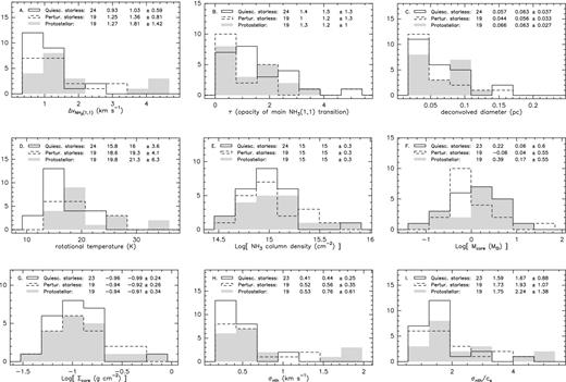
Distributions of: (a) NH3 (1,1) linewidth, (b) opacity, (c) deconvolved diameter, (d) rotational temperature, (e) ammonia column density, (f) core mass Mcore, (g) core surface density Σcore, (h) non-thermal dispersion σnth and (i) non-thermal to thermal velocity dispersion ratio σnth/cs, for quiescent starless (solid line histogram), perturbed starless (dashed line histogram), and protostellar (grey filled histogram) cores. The numbers at the top of each panel are the total number of sources used in the histogram, the median and the mean ± standard deviation values.
Derived parameters for the ammonia cores.
| Tkinb | σthc | σnthc | σtot | Mcored | Σcoree | Mvirf | |||
|---|---|---|---|---|---|---|---|---|---|
| ID | Typea | (K) | (km s−1) | (km s−1) | σnth/cs | (km s−1) | (M⊙) | (g cm−2) | (M⊙) |
| 01 | P | 16.4 | 0.09 | 0.32 | 1.32 | 0.40 | 2.56 | 0.09 | 5.42 |
| 02 | S | 13.3 | 0.08 | 0.51 | 2.36 | 0.56 | 0.90 | 0.11 | 7.19 |
| 03 | P | 18.1 | 0.09 | 0.67 | 2.63 | 0.71 | 0.18 | 0.03 | 10.26 |
| 04 | S* | 17.5 | 0.09 | 0.60 | 2.41 | 0.65 | 0.18 | 0.07 | 5.59 |
| 05 | P? | 12.1 | 0.08 | 0.26 | 1.25 | 0.33 | 1.28 | 0.15 | 2.03 |
| 06 | P | 66.3 | 0.18 | 1.59 | 3.27 | 1.66 | 2.76 | 0.46 | 59.31 |
| 07 | P? | 53.9 | 0.16 | 0.71 | 1.61 | 0.83 | 2.41 | 0.18 | 17.99 |
| 08 | P? | 26.9 | 0.11 | 0.60 | 1.94 | 0.67 | 2.78 | 0.14 | 15.76 |
| 09 | P | 17.4 | 0.09 | 0.56 | 2.27 | 0.62 | 5.57 | 0.18 | 17.10 |
| 10 | P | 21.6 | 0.10 | 0.41 | 1.47 | 0.49 | 0.80 | 0.10 | 4.69 |
| 11 | S | 16.2 | 0.09 | 0.21 | 0.87 | 0.32 | 1.81 | 0.11 | 1.93 |
| 12 | S | 18.5 | 0.09 | 0.40 | 1.56 | 0.47 | 1.58 | 0.12 | 5.80 |
| 13 | S | 14.5 | 0.08 | 0.21 | 0.92 | 0.31 | 0.86 | 0.11 | 1.32 |
| 14 | S | 11.3 | 0.07 | 0.17 | 0.83 | 0.26 | 1.11 | 0.13 | 0.90 |
| 15 | S | 18.9 | 0.10 | 0.16 | 0.63 | 0.31 | 0.67 | 0.06 | 1.16 |
| 16 | P | 31.1 | 0.12 | 0.49 | 1.48 | 0.59 | 2.36 | 0.08 | 13.23 |
| 17 | P? | 21.8 | 0.10 | 0.33 | 1.18 | 0.43 | 1.54 | 0.11 | 4.20 |
| 18 | P | 38.0 | 0.14 | 0.69 | 1.89 | 0.78 | 0.79 | 0.07 | 16.01 |
| 19 | S* | 32.1 | 0.12 | 0.54 | 1.60 | 0.64 | 1.50 | 0.07 | 13.19 |
| 20 | P | 19.7 | 0.10 | 0.20 | 0.77 | 0.33 | 1.90 | 0.11 | 2.05 |
| 21 | S* | 14.6 | 0.08 | 0.17 | 0.76 | 0.28 | 0.35 | 0.10 | 0.66 |
| 22 | S | 15.9 | 0.09 | 0.37 | 1.55 | 0.44 | 3.28 | 0.14 | 6.49 |
| 23 | P | 21.1 | 0.10 | 0.40 | 1.45 | 0.48 | 2.87 | 0.12 | 7.92 |
| 24 | P | 16.8 | 0.09 | 0.25 | 1.04 | 0.35 | 3.62 | 0.15 | 3.42 |
| 25 | S* | 22.5 | 0.10 | 0.49 | 1.75 | 0.57 | 0.91 | 0.13 | 6.54 |
| 26 | S* | 26.6 | 0.11 | 0.17 | 0.56 | 0.35 | 0.28 | 0.04 | 1.10 |
| 27 | P | 34.4 | 0.13 | 1.87 | 5.37 | 1.91 | 1.70 | 0.23 | 90.38 |
| 28 | S* | 36.6 | 0.13 | 1.30 | 3.62 | 1.35 | 0.97 | 0.10 | 49.97 |
| 29 | S | 18.9 | 0.10 | 1.16 | 4.48 | 1.19 | 0.38 | 0.13 | 22.09 |
| 30 | S* | 21.3 | 0.10 | 1.17 | 4.24 | 1.20 | 0.49 | 0.10 | 28.71 |
| 31 | S | 16.9 | 0.09 | 0.67 | 2.72 | 0.71 | 0.64 | 0.15 | 8.92 |
| 32 | P? | 21.8 | 0.10 | 0.89 | 3.21 | 0.93 | 70.21 | 0.35 | 108.66 |
| 33 | S | 22.0 | 0.10 | 0.51 | 1.83 | 0.58 | 7.19 | 0.10 | 22.24 |
| 34 | S | 26.2 | 0.11 | 0.56 | 1.84 | 0.64 | 5.31 | 0.07 | 26.71 |
| 35 | P | 40.5 | 0.14 | 1.98 | 5.23 | 2.01 | 3.72 | 0.91 | 75.60 |
| 36 | S | 17.9 | 0.09 | 0.32 | 1.28 | 0.41 | 14.24 | 0.66 | 4.96 |
| 37 | P? | 19.8 | 0.10 | 0.36 | 1.35 | 0.45 | 11.64 | 0.44 | 6.77 |
| 38 | P | 63.2 | 0.18 | 1.93 | 4.07 | 1.98 | 2.54 | 0.18 | 135.01 |
| 39 | S* | 35.3 | 0.13 | 1.28 | 3.62 | 1.33 | 5.61 | 0.12 | 109.15 |
| 40 | P? | 34.5 | 0.13 | 1.09 | 3.12 | 1.15 | 2.76 | 0.12 | 54.11 |
| 41 | S | 32.5 | 0.13 | 0.55 | 1.61 | 0.64 | 2.55 | 0.07 | 18.66 |
| 42 | S | 27.4 | 0.12 | 0.54 | 1.72 | 0.62 | 2.35 | 0.06 | 17.82 |
| 43 | S | 27.9 | 0.12 | 1.03 | 3.26 | 1.07 | 3.33 | 0.14 | 49.72 |
| 44 | P? | 29.0 | 0.12 | 0.58 | 1.82 | 0.66 | 11.88 | 0.12 | 33.29 |
| 45 | S* | 18.9 | 0.10 | 0.44 | 1.71 | 0.51 | 6.78 | 0.23 | 10.54 |
| 46 | S* | 14.8 | 0.08 | 0.36 | 1.57 | 0.43 | 32.56 | 0.40 | 11.82 |
| 47 | P | 24.9 | 0.11 | 0.90 | 3.02 | 0.94 | 9.81 | 0.21 | 53.15 |
| 48 | P? | 17.8 | 0.09 | 0.42 | 1.68 | 0.49 | 12.15 | 0.21 | 13.55 |
| 49 | P | 20.6 | 0.10 | 0.43 | 1.59 | 0.51 | 4.33 | 0.17 | 9.43 |
| 50 | P? | 16.6 | 0.09 | 0.56 | 2.29 | 0.61 | 10.63 | 0.27 | 18.96 |
| 51 | S* | 19.4 | 0.10 | 0.82 | 3.14 | 0.86 | 1.94 | 0.27 | 17.51 |
| 52 | S* | 22.1 | 0.10 | 0.66 | 2.37 | 0.72 | 0.36 | 0.08 | 9.21 |
| 53 | P? | 26.1 | 0.11 | 0.54 | 1.77 | 0.62 | 0.08 | 0.04 | 4.03 |
| 54 | P | 22.7 | 0.10 | 0.43 | 1.53 | 0.52 | 0.29 | 0.06 | 4.18 |
| 55 | S | 14.3 | 0.08 | 0.29 | 1.28 | 0.37 | 2.59 | 0.14 | 3.75 |
| 56 | S* | 29.7 | 0.12 | 0.40 | 1.24 | 0.52 | 2.11 | 0.06 | 9.62 |
| 57 | S | 15.4 | 0.09 | 0.26 | 1.11 | 0.35 | 3.41 | 0.08 | 4.67 |
| 58 | S | 20.4 | 0.10 | 0.48 | 1.79 | 0.55 | 1.73 | 0.05 | 14.06 |
| 59 | P? | 24.3 | 0.11 | 0.35 | 1.21 | 0.46 | 0.70 | 0.04 | 5.42 |
| 60 | P | 25.2 | 0.11 | 0.60 | 2.00 | 0.67 | 1.85 | 0.05 | 21.32 |
| 61 | S | 18.3 | 0.09 | 0.36 | 1.39 | 0.44 | 0.36 | 0.06 | 3.15 |
| 62 | P? | 20.6 | 0.10 | 0.74 | 2.75 | 0.79 | 0.52 | 0.09 | 12.75 |
| 63 | S | 14.5 | 0.08 | 0.41 | 1.80 | 0.47 | 0.29 | 0.14 | 2.32 |
– continued
| Tkinb | σthc | σnthc | σtot | Mcored | Σcoree | Mvirf | |||
|---|---|---|---|---|---|---|---|---|---|
| ID | Typea | (K) | (km s−1) | (km s−1) | σnth/cs | (km s−1) | (M⊙) | (g cm−2) | (M⊙) |
| 64 | P? | 19.3 | 0.10 | 0.39 | 1.49 | 0.47 | 0.14 | 0.08 | 1.97 |
| 65 | P | 23.7 | 0.11 | 0.46 | 1.60 | 0.55 | 0.11 | 0.07 | 2.76 |
| 66 | S* | 15.7 | 0.09 | 0.39 | 1.67 | 0.46 | 0.41 | 0.11 | 2.92 |
| 67 | S | 15.7 | 0.09 | 0.17 | 0.73 | 0.29 | 0.15 | 0.10 | 0.43 |
| 68 | S | 23.6 | 0.11 | 0.52 | 1.79 | 0.59 | 0.04 | 0.04 | 2.78 |
| 69 | S | 20.1 | 0.10 | 0.26 | 0.96 | 0.37 | 0.20 | 0.09 | 1.05 |
| 71 | S* | 28.2 | 0.12 | 0.55 | 1.75 | 0.64 | 0.85 | 0.15 | 7.25 |
| 72 | S* | 22.0 | 0.10 | 0.18 | 0.65 | 0.33 | 0.81 | 0.13 | 1.04 |
| 73 | S* | 25.1 | 0.11 | 0.61 | 2.06 | 0.68 | 0.47 | 0.17 | 6.11 |
| 74 | P? | 31.9 | 0.12 | 0.36 | 1.07 | 0.49 | 0.42 | 0.09 | 3.05 |
| 75 | S* | 36.6 | 0.13 | 0.30 | 0.85 | 0.47 | 0.81 | 0.07 | 3.60 |
| 76 | S* | 20.7 | 0.10 | 0.29 | 1.07 | 0.40 | 2.19 | 0.35 | 2.25 |
| 77 | P | 25.7 | 0.11 | 0.17 | 0.57 | 0.35 | 0.18 | 0.09 | 0.56 |
aTypes of the core: S: quiescent starless, S*: perturbed starless, P: protostellar, and P?: possible protostellar (see Section 3.1 and Table B1).
bKinetic temperature, in K, derived from the rotational temperature and following Tafalla et al. (2004). We emphasize that Tafalla et al. empirical relation is accurate only for temperatures ≲ 20 K, and thus the kinetic temperature given here should be regarded, for high temperatures, as an approximation.
cThermal (σth) and non-thermal (σnth) velocity dispersion, in km s−1.
dMass of the core derived as Mcore = (N/X)μmHA, with μ (= 2.8) the mean molecular mass per H molecule, A (= π(size/2)2) the area and assuming an abundance of NH3 with respect to H2 (X) for all the cores of 4.2 × 10⁻⁸ (e.g. Pillai et al. 2006; Foster et al. 2009; Friesen et al. 2009; Rygl et al. 2010; Chira et al. 2013).
eCore mass surface density derived as Σcore = Mcore/A.
fVirial mass derived from Mvir = 210 [R/pc] [Δv/kms−1]2 M⊙ assuming uniform density across the core (MacLaren, Richardson & Wolfendale 1988; Estalella et al. 1993). R is the radius of the core (obtained from the diameter size listed in Table 3), and Δv is the intrinsic linewidth of the NH3 (1,1) line (listed in Table 3).
| Trot | Tkin | Size | τ | |$N_\mathrm{NH_3}$| | Mcore | Σcore | ΔV(1, 1) | σnth | σnth/cs | Mvir | |
|---|---|---|---|---|---|---|---|---|---|---|---|
| Core type | (K) | (K) | (pc) | (cm−2) | (M⊙) | (g cm−2) | (km s−1) | (km s−1) | (M⊙) | ||
| Quiescent starless | 16.0 | 18.8 | 0.063 | 1.5 | 1015.0 | 1.15 | 0.10 | 1.03 | 0.44 | 1.67 | 5.1 |
| Perturbed starless | 19.3 | 24.2 | 0.056 | 1.2 | 1015.0 | 1.09 | 0.12 | 1.36 | 0.56 | 1.93 | 7.0 |
| Protostellar | 21.3 | 28.8 | 0.063 | 1.2 | 1015.0 | 1.47 | 0.12 | 1.81 | 0.76 | 2.24 | 11.7 |
| All sample | 18.8 | 23.8 | 0.065 | 1.4 | 1015.0 | 1.36 | 0.12 | 1.36 | 0.57 | 1.91 | 7.8 |
Parameters derived for the clumps associated with the 15 massive star-forming regions.
| Sνb | Massc | FWHMd | Diameterd | Σclumpe | |
|---|---|---|---|---|---|
| No.a | (Jy) | (M⊙) | (arcsec) | (arcsec)/(pc) | (g cm−2) |
| 1. | 1.2 | 85 | 32.4 | 30.5/0.27 | 0.32 |
| 2. | 15.3 | 278 | 28.7 | 25.1/0.22 | 1.55 |
| 3. | 6.8 | 123 | 44.2 | 41.9/0.37 | 0.25 |
| 4. | 21.1 | 384 | 40.2 | 37.7/0.33 | 0.94 |
| 5. | 4.5 | 64 | 30.1 | 26.6/0.21 | 0.40 |
| 6. | 7.3 | 199 | 31.9 | 28.7/0.31 | 0.57 |
| 7. | 32.9 | 1160 | 30.0 | 26.5/0.32 | 2.97 |
| 8. | 13.3 | 201 | 34.5 | 31.5/0.25 | 0.85 |
| 9. | 28.3 | 2290 | 37.8 | 35.1/0.65 | 1.46 |
| 10. | 15.2 | 341 | 45.0 | 42.8/0.42 | 0.53 |
| 11. | 15.8 | 174 | 56.5 | 54.7/0.37 | 0.34 |
| 12. | 6.7 | 253 | 38.5 | 35.9/0.45 | 0.33 |
| 13. | 4.5 | 145 | 34.6 | 31.6/0.37 | 0.29 |
| 14. | 5.2 | 17 | 16.5 | 8.8/0.03 | 4.30 |
| 15. | 67.1 | 185 | 41.6 | 39.2/0.13 | 2.78 |
aNumber of the region as indicated in Table 1.
bFlux density at 850 μm obtained from the SCUBA Legacy Project (Di Francesco et al. 2008), except for: 00117+6412 (region 1: 1.2 mm from IRAM 30 m; Sánchez-Monge et al. 2008); 20081+3122 (region 7: 850 μm from JCMT; Thompson et al. 2006); 22198+6336 (region 14: 850 μm from JCMT; Jenness, Scott & Padman 1995).
cMass of the clump measured from the JCMT at 850 μm or the IRAM 30 m at 1.2 mm, assuming a dust temperature of 20 K, a dust (+gas) mass opacity coefficient of 0.0175 cm2 g−1 at 850 μm and 0.0090 cm2 g−1 at 1.2 mm (Ossenkopf & Henning 1994), and a gas-to-dust mass ratio of 100.
dObserved diameter at FWHM obtained from a Gaussian fit, and deconvolved diameter derived taking into account a main beam for the SCUBA observations at 850 μm of 14 arcsec. Our sizes obtained from a Gaussian fit are slightly different from those reported by Palau et al. (2013), which were estimated by measuring the observed diameter directly on the image, and using a beam size of 23 arcsec for deconvolution, which affects mainly the sources with the smallest sizes.
eClump mass surface density derived as Σclump = mass/area with area = π (diameter/2)2.
Values of Δ(m, α) for calculating the parameter uncertainties, where m is the number of fitted parameters simultaneously, and α is the significance level, given in per cent and in the equivalent number of sigmas for a Gaussian error distribution.
| α | ||||
|---|---|---|---|---|
| 68.23 per cent | 90.00 per cent | 99.00 per cent | 99.90 per cent | |
| m | (1σ) | (1.64σ) | (2.57σ) | (3.30σ) |
| 1 | 1.00 | 2.71 | 6.64 | 10.83 |
| 2 | 2.30 | 4.60 | 9.21 | 13.82 |
| 3 | 3.53 | 6.25 | 11.34 | 16.27 |
| 4 | 4.72 | 7.78 | 13.28 | 18.46 |
| 5 | 5.89 | 9.24 | 15.09 | 20.52 |
| 6 | 7.04 | 10.64 | 16.81 | 22.46 |
| 7 | 8.17 | 12.02 | 18.48 | 24.32 |
| 8 | 9.30 | 13.36 | 20.09 | 26.12 |
| 9 | 10.42 | 14.68 | 21.67 | 27.87 |
| 10 | 11.53 | 15.99 | 23.21 | 29.59 |
From the ammonia column density (listed in Table 3), we derived the mass of the core and the core mass surface density, following the procedures explained in the footnotes of Table 4. These two quantities are listed in Columns 8 and 9 of Table 4, and their distributions are shown in panels F and G of Fig. 2. Starless and protostellar cores show similar mean masses (∼1.0–1.8 M⊙) and mean surface densities (∼0.10–0.12 g cm−2) (see Table 5).
Ammonia correlations
As presented in Section 3.2, we note some differences in the parameters derived for the starless and protostellar cores. In particular, an increase in the temperature and linewidth as we move towards more evolved objects (protostellar cores). In a search for a physical relation between the derived parameters, we plotted several quantities against others, shown as six scattered plots in Fig. 3. In these plots we show the distribution of starless and protostellar core samples in red circles and blue stars, respectively. We performed some statistical tests to search for possible correlations between the physical quantities. In the top right corner of each plot, we give Kendall's τ rank correlation coefficient and the Pearson correlation coefficient (ρ) to a least-squares fit (dotted lines). We find that in five of the six plots there is a possible correlation, with τ coefficients ∼0.3, and ρ in the range 0.4–0.6.
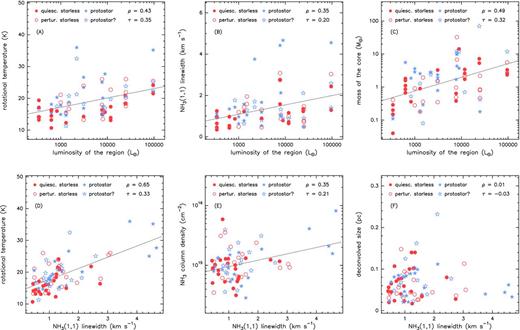
Scatter plots showing the correlations with respect to the bolometric luminosity of (a) the rotational temperature, (b) the NH3 (1,1) linewidth and (c) the core mass, in the top panels; and the correlations with respect to the linewidth of (d) the rotational temperature, (e) the ammonia column density and (f) the core diameter. ‘Quiescent starless’ and ‘perturbed starless’ cores are shown in red filled and open circles, respectively; while ‘protostellar’ and ‘tentatively protostellar’ cores are shown as blue filled and open stars, respectively (see Section 3.1 for details). The black dotted lines show the result of least-squares fits to the data (see Section 3.3), with the Pearson correlation coefficient (ρ) shown in the top right corner, together with Kendall's τ correlation coefficient.
In the top panels of Fig. 3, we show the relation between the temperature, the linewidth and the mass of the core with the bolometric luminosity of the region, while in the bottom panels, we compare the temperature, the ammonia column density and the size of the core with the observed linewidth. We note that we are not able to derive a bolometric luminosity for each individual ammonia core but a single luminosity of the whole region.5 Thus, the plots in Fig. 3 must be interpreted as a correlation between the properties of the cores within a region with respect to the luminosity of the region (which is in general dominated by the brightest mid-IR source). We find a correlation in five of the six panels (panels A to E of Fig. 3). Similar trends between the same parameters have been reported from single-dish observational studies (e.g. Churchwell, Walmsley & Cesaroni 1990; Myers, Ladd & Fuller 1991; Jijina, Myers & Adams 1999; Rygl et al. 2010; Urquhart et al. 2011; Sepúlveda et al. 2011). Our correlations found in ammonia at higher angular resolution thus confirm that these relations take place also at the smaller spatial scales (∼0.05 pc) of individual cores, and are not an observational (average) artefact due to the poor angular resolution of single-dish observations when studying clumps of sizes ∼0.1–10 pc. It is worth noting that in panel B (linewidth versus luminosity) there are four cores with linewidths ∼4 km s−1, located well above the trend found for the other cores. These four cores (AFGL 5142–1; 19035+0641–1; 20126+4104–1; G75.78+0.34–1) are known to be associated with powerful outflows that could perturb the motions of the dense gas close to the powering source (see Zhang et al. 2002; Cesaroni et al. 2005; Sánchez-Monge 2011; Sánchez-Monge et al. 2013). Finally, in panel F, we investigate a possible relation between the size of the core and its linewidth. Since the publication of the Larson's scaling relations (Larson 1981), several authors (e.g. Myers, Linke & Benson 1983; Caselli & Myers 1995; Pirogov et al. 2003) found, from single-dish studies, that larger dense cores have broader lines, as expected in virialized cores. In our sample, however, we find no correlation (with τ = −0.03 and ρ = 0.01) between these two quantities. A possible explanation for this could be that a number of cores suffer an important injection of turbulence, e.g. from the passage of powerful outflows, which should affect the gas motions of the cores only at the scales of our sample (∼0.05 pc; see e.g. Palau et al. 2007b; Liu, Ho & Zhang 2010; Nakamura & Li 2011), and is diluted at the larger scales studied in single-dish observations. Alternatively, the large linewidths might indicate that the cores are collapsing. In Section 4.2, we discuss in more detail the dynamics of the cores in our sample, and relate it to previous single-dish studies.
DISCUSSION
Temperature of the gas and IR radiation
In Section 3.3, we reported a correlation between the temperature of the cores and the luminosity of the region (see Fig. 3 panel A). These higher temperatures can result from various heating processes: (i) feedback from low-mass stars, e.g. molecular outflows, as found in some cores of AFGL 5142 or 20293+5932 (e.g. Zhang et al. 2002; Palau et al. 2007b); (ii) shocks from convergent flows (e.g. Csengeri et al. 2011a; Beltrán et al. 2012); (iii) feedback from high-mass stars, e.g. strong radiation (e.g. Li et al. 2003). In the following, we test the feedback from massive stars as a possible agent for the increase of temperature in the dense cores.
Our interferometric observations permit the study of the spatial distribution of the cores, and their physical properties, with respect to e.g. the (strong) infrared sources and hence the massive stars. In our regions, the bolometric luminosity is generally dominated, at mid-infrared (MIR) and far-infrared (FIR) wavelengths, by a single strong source associated with the most massive star. We assume that the main source of radiation that can heat the surrounding gas is the massive star detectable in the MIR. To determine if there is a relation between the temperature of the cores and the proximity of the MIR source, we searched the MSX Point Source Catalog (Price et al. 1999) for the coordinates of the MIR sources and calculated the MSX to NH3 core separation (|$\Delta _\mathrm{MIR-NH_3}$|; using the coordinates listed in Table 3 for our cores). Using the luminosity and position of the most massive (radiating dominant) source and the separation to each ammonia dense core, we derived the incident flux received by each core as |$L_\mathrm{bol}/(4\pi (\Delta _\mathrm{MIR-NH_3})^2)$|. Note that we are measuring a projected separation, which is a lower limit to the true separation. Thus, for all cores, we actually have an upper limit on the received flux, which affects the absolute normalization of the derived relation and increases the scatter of the data points in this relation. In Fig. 4, we plot the received flux versus the rotational temperature. If the radiation of the most massive star dominates the heating of its surroundings, we expect that the cores closer to the most massive source, i.e. with a large received flux, will have higher temperatures. This is consistent with the trend shown in Fig. 4, where the highest temperatures correspond to the cores with a higher received flux. The black solid line corresponds to the relation |$L_\mathrm{bol}/(4\pi (\Delta _\mathrm{MIR-NH_3})^2)=\sigma _\mathrm{SB}\,T_\mathrm{rot}^4$|, with σSB the Stephan–Boltzmann constant, while the dotted line corresponds to a least-squares fit with a correlation coefficient of 0.6. For a given bolometric luminosity, the temperature is a factor of approximately three times lower for a core located at a distance ∼0.5 pc, than for a similar core located at <0.05 pc.

Received flux for each ammonia core versus the rotational temperature (see Section 4.1 for details). The dotted line shows a least-squares fit to the data, and the solid line corresponds to the relation |$L_\mathrm{bol}/(4\pi (\Delta _\mathrm{MIR-NH_3})^2)=\sigma _\mathrm{SB}T_\mathrm{rot}^4$|, with σSB the Stephan–Boltzmann constant. Symbols are as in Fig. 3.
Summarizing, the radiation deposited in the environment by the most luminous star of the cluster can be responsible for the temperatures measured in the cores of our clustered regions. Thus, the large temperatures measured for our starless cores, in comparison with the temperatures measured in low-mass star-forming regions, can be interpreted as external heating by the radiation of the most massive (forming) stars of the cluster.
Dynamical state of the cores
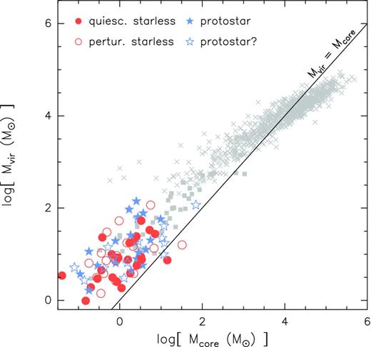
Scatter plot showing the relation between the virial mass Mvir (derived as Mvir = 210 R Δv2; MacLaren et al. 1988) and the mass of the core Mcore. Blue-star and red-circle symbols correspond to the protostellar and starless cores studied in this work (symbols as in Fig. 3). Grey squares correspond to single-dish ammonia data (Sepúlveda et al. 2011) and grey crosses correspond to 13CO single-dish data (Roman-Duval et al. 2010). The solid line corresponds to virialized cores with Mvir = Mcore.
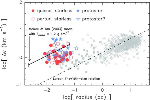
Variation of the linewidth, Δv, with core radius, following Csengeri et al. (2011b). Red and blue symbols correspond to the VLA ammonia data shown in this paper (see Fig. 3 for details), grey squares correspond to single-dish ammonia data (Sepúlveda et al. 2011), and grey crosses correspond to 13CO single-dish data (Roman-Duval et al. 2010). The dashed line indicates a Larson-like linewidth–size relation (Δv ∝ size0.38). The thick solid line corresponds to the turbulent regulated quasi-static model (McKee & Tan 2003), with a surface mass density of 1.3 g cm−2 and a core mass of 0.1 to 100 M⊙ (each interval corresponds to 0.1, 1, 10 and 100 M⊙). The black cross marks the mean and dispersion values of the linewidth (1.36 ± 0.93 km s−1) and radius (0.032 ± 0.019 pc) for the cores studied in this work.
CONCLUSIONS
We present the results of VLA observations of the NH3 (1,1) and (2,2) inversion transition lines towards a sample of 15 massive star-forming regions. We obtained an average spatial resolution of ∼0.05 pc, and analysed the ammonia emission in a consistent way. Our main conclusions can be summarized as follows.
We identified a total of 73 ammonia dense cores using the two-dimensional CLUMPFIND algorithm. On average we found of the order of 5–6 cores in each field (of ∼2 arcmin, or 1.5 pc at a distance of 2.5 kpc), with sizes ∼0.06 pc. The cores were classified as quiescent starless, perturbed starless and protostellar based on its association with infrared emission and taking into account other star formation signposts (e.g. outflows, masers, centimetre continuum emission) reported in the literature.
The average values of linewidth, opacity, rotational temperature and ammonia column density for the 73 dense cores are ∼1.4 km s−1, 1.4, 19 K and 1015 cm−2, respectively. We found that protostellar cores have larger temperatures and linewidths (∼21.3 K and 1.8 km s−1) than quiescent starless cores (∼16.0 K and 1.0 km s−1). Similarly, cores classified as perturbed starless have temperatures and linewidths (∼19.3 K and 1.4 km s−1) slightly larger than quiescent starless cores, but smaller than cores harbouring a protostar.
The average temperatures derived for the quiescent starless cores in our clustered regions (∼16 K) are larger than those measured in starless cores in more isolated regions (∼10 K). Our starless and protostellar cores show important non-thermal supersonic components (σnth ∼ 0.44 km s−1 and 0.76 km s−1, respectively) and σnth/cs ∼ 2.0, well above to the close-to-thermal lines measured in isolated star-forming regions.
We found that the temperature and NH3 (1,1) linewidth of the cores are correlated with the luminosity of the region, suggesting that the feedback of the luminous massive (forming) stars can affect the surrounding molecular environment.
We evaluated a possible relation between the temperature of the core and its separation with the most important radiating source in the region in terms of the incident flux received by the core. The highest temperatures are measured for those cores located close to the brightest MIR source (separations <0.05 pc), with the temperature decaying by a factor of ∼3 when the cores are located at distances ∼0.5 pc. Thus, the large temperatures found in starless cores in massive star-forming regions can be interpreted as external heating by the radiation of the most massive star of the cluster.
We compared the virial masses of our cores (at scales ∼0.05 pc) with those of clumps with sizes ∼0.1–10 pc. A simple virial equilibrium analysis seems to suggest a trend between Mvir and core/clump masses favouring a scenario of a self-similar, self-gravitating, virialized hierarchy of structures from clumps to cores. A closer inspection of the dynamical state at core scales, taking into account external pressure (McKee & Tan 2003), indicates that either another form of support (e.g. from magnetic field) is required to stabilize the cores, or that the cores are close to collapse or even collapsing.
Overall, our data suggest that the cores forming in clustered environments harbouring intermediate-/high-mass stars are more affected/perturbed than cores in clustered low-mass star-forming regions, and thus the initial conditions for star formation in these environments seem to be different to those typically assumed in low-mass star-forming regions.
We are grateful to James di Francesco for support with SCUBA data. We thank the anonymous referee for his/her constructive criticisms. The figures of this paper have been done in GREG of the gildas software package developed at the Institut de Radioastronomie Millimétrique (IRAM) and the Observatoire de Grenoble. AP is supported by a JAE-Doc CSIC fellowship co-funded with the European Social Fund under the programme ‘Junta para la Ampliación de Estudios’, by the Spanish MICINN grant AYA2011-30228-C03-02 (co-funded with FEDER funds), and by the AGAUR grant 2009SGR1172 (Catalonia). GB is funded by an Italian Space Agency (ASI) fellowship under contract number I/005/11/0.
The VLA is operated by the National Radio Astronomy Observatory (NRAO). The NRAO is a facility of the National Science Foundation operated under cooperative agreement by Associated Universities, Inc.
The Wide-filed Infrared Survey Explorer (WISE) is described in Wright et al. (2010).
The differentiation between quiescent and perturbed starless cores was already introduced in Fontani et al. (2011).
To estimate the bolometric luminosity Lbol (listed in Table 1), we compiled the flux densities at different frequencies from 2MASS (Skrutskie et al. 2006), Spitzer/IRAC+MIPS, WISE, MSX, IRAS and James Clerk Maxwell Telescope (JCMT) (SCUBA; Di Francesco et al. 2008) catalogues and followed the methodology explained in Palau et al. (2013).
Note that the offset seen in Fig. 5 cannot be easily explained in terms of the uncertainties of the observational quantities involved in the plot. The two main sources of uncertainty are the ammonia abundance and the linewidth. For the ammonia abundance we assumed a mean value of (4.2 ± 2.7) × 10−8. This value is obtained from different surveys (Pillai et al. 2006; Foster et al. 2009; Friesen et al. 2009; Rygl et al. 2010; Chira et al. 2013), over a total of 122 clumps of different star-forming regions. Thus, we expect an uncertainty of ∼60 per cent for the mass of the core. The linewidth is obtained from the spectral line fit described in Section 3.2, which provides errors of a few tenths of km s−1, corresponding to a 10–30 per cent uncertainty in linewidth. These observational errors alone are expected to affect the data randomly instead of introducing a systematic offset, and thus are not likely the cause of the observed offset of about one order of magnitude.
HfS is freely available and can be downloaded from http://www.am.ub.edu/~robert/hfs/hfs.html
REFERENCES
APPENDIX A: HYPERFINE STRUCTURE (HfS) FITTING
Parameters of the fit
The usual fitting of the hyperfine structure of a transition, for instance, the inversion transition NH3 (J, K) = (1, 1), estimates four free parameters of the transition, namely
τm, the optical depth of the main component,
A × τm, product of the amplitude (A = f [Jν(Tex) − Jν(Tbg)],
where f is the filling factor, Jν(T) is the Planck function in units of temperature, Tex is the excitation temperature and Tbg is the background temperature) times the optical depth of the main component,
vLSR, the central velocity of the main component, and
Δv, the linewidth of the hyperfine components,
with the usual assumptions that Tex, vLSR and Δv are the same for all the hyperfine components.
However, some of the parameters are ill-conditioned in some cases. In the optically thin limit, τm ≪ 1, only an upper limit for the value of τm can be obtained. However, the parameter A × τm gives the peak intensity of the line (provided that the hyperfine components are unresolved, or, in the case NH3, the hyperfine magnetic components that form part of the main component), and is well constrained. This parameter, in the Rayleigh–Jeans approximation, is necessary to calculate the column density of emitting molecules. In the optically thick limit, τm ≫ 1, only lower limits for τm and A × τm can be obtained (and consequently, a lower limit for the column density).
A better fit parameter than τm, with well-defined values in the optically thin and optically thick limits, is |$1-e^{-\tau _m}$|. This parameter always has values between 0 (optically thin limit, τm ≪ 1) and 1 (optically thick limit, τm ≫ 1). Similarly, |$A\left(1-e^{-\tau _m}\right)$| is a better fit parameter than A × τm, since it is well constrained in all cases.
The Hyperfine Structure7 (hereafter HfS) fitting procedure used to fit the NH3 (J, K) = (1, 1) lines in this paper fits the four parameters
|$1-e^{-\tau _m}$|,
|$A\left(1-e^{-\tau _m}\right)$|,
vLSR,
Δv.
The values and uncertainties for the parameters needed to derive physical properties of the emitting gas, τm and A × τm (or their limits in the two limiting cases) can be easily derived from the values and uncertainties for the parameters of the fit.
Fitting procedure
Several sampling methods of the m-dimensional parameter space are possible, i.e. regular grid, random, Halton sequence (Halton 1964). We adopted a Halton quasi-random sequence because it samples the parameter space more evenly than a purely random sequence, and the convergence of the fitting procedure to the minimum of χ2 is faster.
Parameter error estimation
Once the best-fitting parameter values for which |$\chi ^2=\chi ^2_\mathrm{min}$| are found, the uncertainty in the fitted parameters, σ(pk), (k = 1 …m), can be estimated as the projection over each parameter axis of the confidence region of the parameters, the region of the m-dimensional parameter space for which χ2 does not exceed the minimum value by a certain amount, |$\chi ^2_\mathrm{min}+\Delta$|.
APPENDIX B: VELOCITY, LINEWIDTH AND SPECTRA IMAGES
In Table B1, we summarize the infrared properties of each core, together with the information of other star formation signposts reported in the literature. In Column 4 of the table, we classify each core as ‘quiescent starless’ (S), ‘perturbed starless’ (S*), ‘protostellar’ (P) or ‘tentatively protostellar’ (P?).
Classification of ammonia cores in protostellar or starless.
| ID regiona | No. | Typeb | IRAC | MIPS/WISE | mm | cm | Outflow | Maser | Comments |
|---|---|---|---|---|---|---|---|---|---|
| 01 00117+6412 | 01 | P | Point | – | Yes | No | No | No | |
| 02 | 02 | S | Dark | – | Yes | No | No | No | |
| 03 | 03 | P | Point | Yes | Yes | Yes | Yes | Yes | |
| 04 | 04 | S* | Dark | – | Yes | No | No | Yes | |
| 05 | 05 | P? | Point | – | No | No | No | No | No mm/outflow/maser associated |
| 06 AFGL5142 | 01 | P | Point | Yes | Yes | Yes | Yes | Yes | |
| 07 | 02 | P? | Point | – | No | No | OA | No | Core along outflow axis |
| 08 | 03 | P? | Point | – | No | No | No | No | |
| 09 05345+3157NE | 01 | P | Point | – | Yes | Yes | No? | No | |
| 10 | 02 | P | Point | Yes | Yes | No | Yes | Yes | |
| 11 | 03 | S | Dark | – | No | No | No | No | |
| 12 | 04 | S | Dark? | Yes? | Yes | No | No | No | Point IR source at the border, but dark |
| 13 | 05 | S | Dark | – | Yes | No | No | No | |
| 14 | 06 | S | Dark | – | Yes | No | No | No | |
| 15 | 07 | S | Dark | – | No | No | No | No | |
| 16 05358+3543NE | 01 | P | Ext? | – | Yes | No | Yes | No | |
| 17 | 02 | P? | Point | – | No | No | OA | No | Core along outflow axis |
| 18 | 03 | P | Point | Yes | Yes | Yes | Yes | Yes | |
| 19 | 04 | S* | Dark | – | No | No | OA | No | Near CO outflow lobe |
| 20 | 05 | P | Point | – | No | No | Yes | No | |
| 21 | 06 | S* | Dark | – | No | No | OA | No | Near SiO outflow lobe |
| 22 | 07 | S | Dark | – | No | No | No | No | |
| 23 05373+2349 | 01 | P | Point | – | Yes | Yes | Yes | No | |
| 25 | 02 | S* | Dark? | Yes? | Faint | No | No | No | Between two strong IR sources |
| 27 19035+0641 | 01 | P | Point | Yes | Yes | ||||
| 28 | 02 | S* | Dark | – | No | Close to bright IRAC source | |||
| 29 | 03 | S | Dark | – | No | ||||
| 30 | 04 | S? | Ext | – | No | ||||
| 31 | 05 | S | Dark | – | No | ||||
| 32 20081+3122 | 01 | P? | Point | – | Yes? | No | OA | No | mm source 4 arcsec to the south of the polygon |
| 33 | 02 | S | Dark | – | No | No | No | No | |
| 35 20126+4104 | 01 | P | Point | Yes | Yes | Yes | Yes | Yes | |
| 36 | 02 | S | Dark | – | Yes | No | No | No | |
| 37 | 03 | P? | Point | – | No | No | No | No | |
| 38 G75.78+0.34 | 01 | P | Point | Yes | Yes | Yes | Yes | Yes | |
| 39 | 02 | S* | Ext | – | No | No | No | No | Near strong IRAC source |
| 40 | 03 | P? | Point | – | No | No | No | No | |
| 41 | 04 | S | Dark | – | No | No | No | No | |
| 43 | 05 | S | Dark | – | No | No | No | No | |
| 44 | 06 | P? | Point | – | No | No | No | No | |
| 45 20293+3952 | 01 | S* | Dark? | – | No | No | No | No | Near strong IRAC source |
| 46 | 02 | S* | Dark? | – | Yes | No | OA | No | Perturbed by outflow |
| 47 | 03 | P | Point | Yes | Yes | No | Yes | Yes | |
| 48 | 04 | P? | Point | – | Yes | No | No | No | |
| 49 | 05 | P | Point | Yes | Yes | No | Yes | No | |
| 50 | 06 | P? | Point | – | No | No | |||
| 51 20343+4129 | 01 | S* | ext | – | Yes | No | No | No | Near strong IRAC source, perturbed? |
| 52 | 02 | S* | Dark | – | Yes | No | OA? | No | Near strong IRAC source, perturbed? |
| 53 | 03 | P? | Dark? | – | Yes | Yes? | OA? | No | Near strong IRAC source, perturbed? |
| 54 | 04 | P | Point | Yes | faint | Yes | No | No | |
| 55 22134+5834 | 01 | S | Dark | – | No | No | |||
| 56 | 02 | S* | Dark? | – | No | No | Near strong IRAC source, perturbed? | ||
| 57 | 03 | S | Dark | – | No | No | |||
| 58 | 04 | S | Dark | – | no | No | |||
| 59 | 05 | P? | Point | – | No | No | |||
| 60 22172+5549N | 01 | P | Point | Yes | Yes | No | Yes | No | |
| 61 | 02 | S | Dark | – | No | No | No | No | |
| 62 | 03 | P? | Point | Yes | Faint | No | OA | No | Core along outflow axis |
| 63 22198+6336 | 01 | S | Dark | – | No | No | No | No | |
| 64 | 02 | P? | Point | – | No | No | No | No | |
| 65 | 03 | P | Point | Yes | Yes | Yes | Yes | Yes |
– continued
| ID regiona | No. | Typeb | IRAC | MIPS/WISE | mm | cm | Outflow | Maser | Comments |
|---|---|---|---|---|---|---|---|---|---|
| 66 | 04 | S* | Ext | – | No | No | OA | No | Core along outflow axis |
| 67 | 05 | S | Dark | – | No | No | No | No | |
| 68 | 06 | S | Dark | – | No | No | No | No | |
| 69 | 07 | S | Dark | – | Yes | No | No | No | |
| 70 | 08 | S | Dark | – | No | No | |||
| 71 CepA | 01 | S* | Dark | – | No | OA | No | Core close to outflow axis | |
| 72 | 02 | S* | Dark | – | No | No | No | ||
| 73 | 03 | S* | Dark | – | No | OA | No | Core close to outflow axis | |
| 74 | 04 | P? | Point | – | No | OA | No | Core close to outflow axis | |
| 75 | 05 | S* | Ext | – | No | OA | No | Core close to outflow axis | |
| 76 | 06 | S? | Ext | – | No | No | No | ||
| 77 | 07 | P | Point | Yes | No | OA | No | Core close to outflow axis |
aReferences: we have made use of the Spitzer/IRAC, Spitzer/MIPS and WISE images to characterize the IR properties of the cores at wavelengths ranging from 3.6 to 24 μm. For each region we have searched the literature for information on millimetre continuum, centimetre continuum, outflow and maser emission. The references used (for each region) are:
AFGL5142: Zhang et al. (2002, 2007); Busquet (2010); Sánchez-Monge (2011); Busquet et al. (2011); Palau et al. (2011, 2013);
05373+2349: Rodriguez et al. (1980); Varricatt et al. (2010); Molinari et al. (1996, 2002, 2008); Gutermuth et al. (2009); Khanzadyan et al. (2011);
19035+0641: Sánchez-Monge (2011);
20293+3952: Beuther et al. (2002c), Beuther, Schilke & Gueth (2004a), Beuther, Schilke & Wyrowski (2004b), Busquet et al. (2010), Palau et al. (2007a);
bType of the core: S: quiescent starless, S*: perturbed starless, P: protostellar, P?: tentatively protostellar (see Section 3.1).
In Fig. B1, we present the first-order (intensity-weighted mean vLSR) and second-order (intensity-weighted mean linewidth) moment maps for the 15 massive star-forming regions studied in this work. Note that the second-order moment maps have been corrected to show directly the linewidth (Δv) instead of the dispersion (σv) by using the relation |$\Delta v = \sqrt{8\ln 2}\,\sigma _v$|.
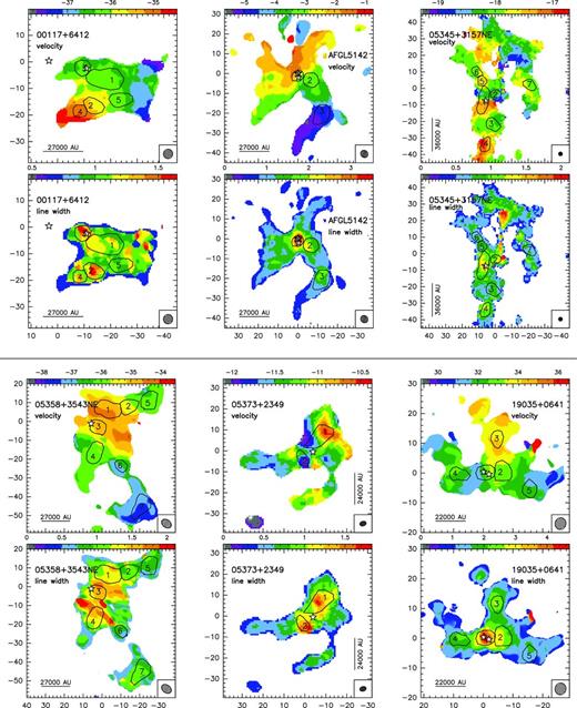
Velocity and linewidth maps (in units of km s−1) obtained from the first- and second-order moment maps. Note that the second-order moment map has been multiplied by |$\sqrt{8\,\ln 2}$| to obtain linewidth instead of dispersion. For each region we show two panels corresponding to the intensity-weighted mean vLSR (top panel) and to the intensity-weighted mean velocity linewidth (bottom panel). Colour scales are indicated in the top of each panel. Symbols are as in Fig. 1.
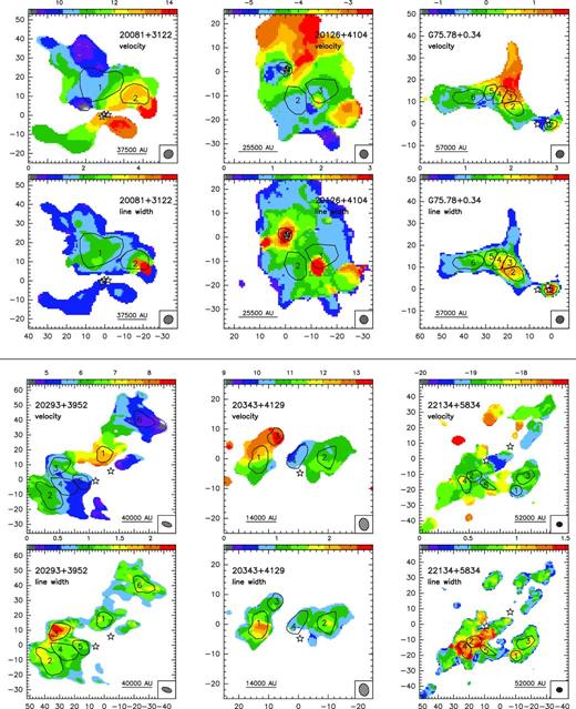
– continued
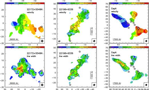
– continued
In Fig. B2, we present the observed and fitted spectra of the NH3 (1,1) and NH3 (2,2) transitions for all the cores identified and listed in Table 3.
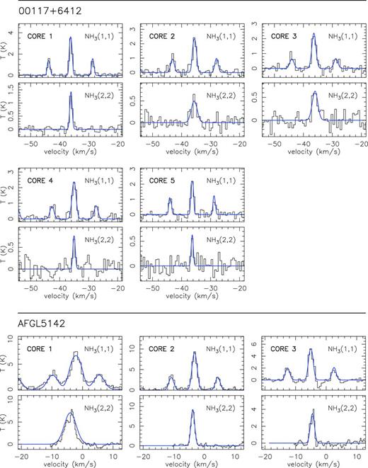
Observed (black histogram) and fitted (thick blue line) spectra of the NH3 (1,1) and (2,2) lines for the cores listed in Table 3. Vertical axis corresponds to brightness temperature (in K), and horizontal axis corresponds to velocity (in km s−1).
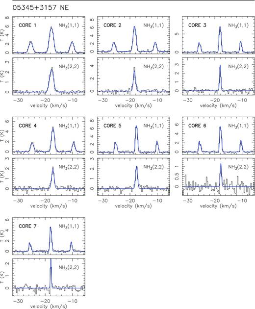
– continued
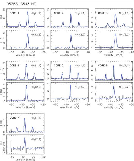
– continued
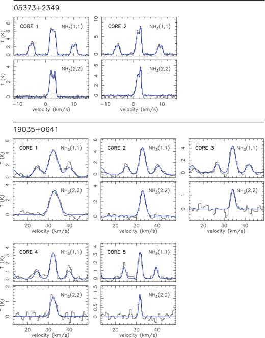
– continued
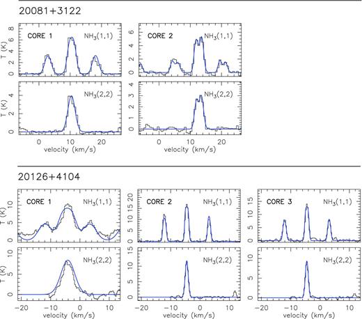
– continued
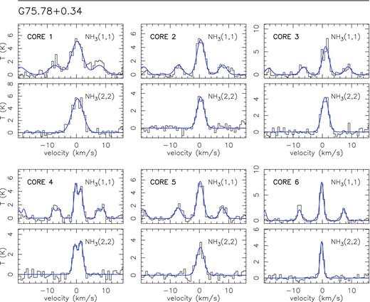
– continued
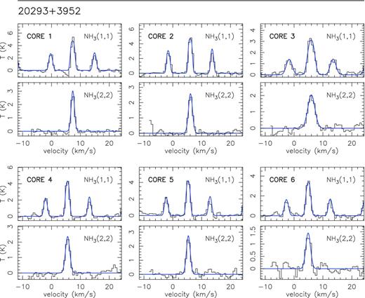
– continued
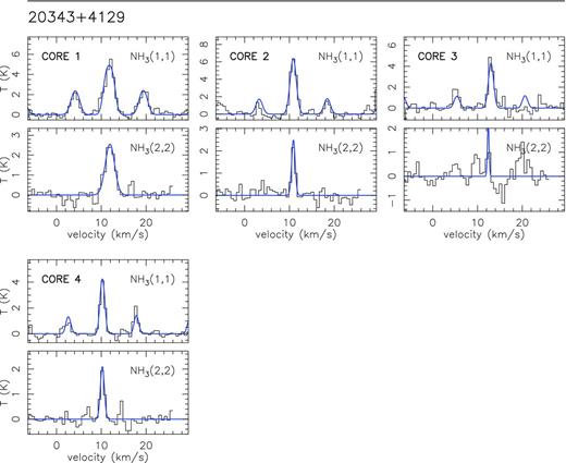
– continued
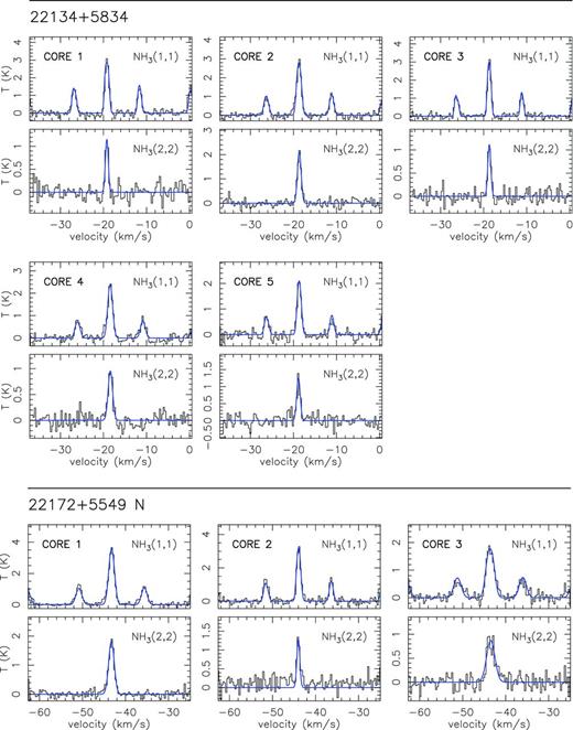
– continued

– continued
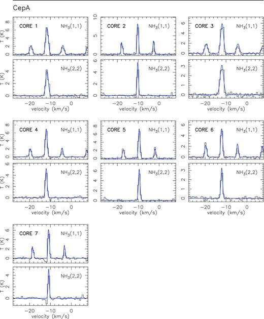
– continued
