Abstract
The possibility that we live in a special place in the universe, close to the centre of a large, radially inhomogeneous void, has attracted attention recently as an alternative to dark energy or modified gravity to explain the accelerating universe. We show that the distribution of orientations of galaxy pairs can be used to test the Copernican principle that we are not in a central or special region of Universe. The popular void models cannot fit both the latest Type Ia supernova, cosmic microwave background data and the distribution of orientations of galaxy pairs simultaneously. Our results rule out the void models at the 4σ confidence level as the origin of cosmic acceleration and favour the Copernican principle.
INTRODUCTION
The standard model of cosmology based on the cosmological principle (homogeneity, isotropy, validity of General Relativity) which contains about 23 per cent dark matter, 4 per cent ordinary matter and 73 per cent dark energy driving the acceleration of a flat universe has been established. Many astronomical observations support this standard picture, including Type Ia supernovae (SNe Ia; Riess et al. 1998; Perlmutter et al. 1999), cosmic microwave background (CMB; Komatsu et al. 2011; Sherwin et al. 2011), baryon acoustic oscillations (BAO; Eisenstein et al. 2005) and gamma-ray bursts (Dai, Liang, Xu 2004; Wang, Dai & Zhu 2007; Wang, Qi & Dai 2011).
In the meanwhile, the inhomogeneous Lemaître–Tolman–Bondi (LTB; Lemaître 1933; Tolman 1934; Bondi 1947) universe could also induce an apparent dimming of the light of distant supernovae. The idea is to drop the dark energy and the Copernican principle, and instead suppose that we are near the centre of a large, non-linearly underdense, nearly spherical void surrounded by a flat, matter-dominated Einstein-de Sitter (EdS) space–time. Because the observer must be at the centre of void, so the LTB models violate the Copernican principle. Because of the observed isotropy of the CMB, the observer must be located very close to the centre of the void (Alnes & Amarzguioui 2006). It was demonstrated that the LTB models can fit the SNe Ia data, as well as the BAO data and the CMB data (Garcia-Bellido & Haugboelle 2008). Some tests have actually been proposed: the Goodman–Caldwell–Stebbins test, which looks at the CMB inside our past lightcone (Goodman 1995; Caldwell & Stebbins 2008), the curvature test, which is based on the tight relation between curvature and expansion history in a Friedmann space–time (Clarkson, Bassett & Lu 2008), and the radial and transverse BAO scale (Zibin et al. 2008; Garcia-Bellido & Haugboelle 2009). However, based on these tests, void models have not yet been ruled out (Clifton, Ferreira & Land 2008; Uzan, Clarkson & Ellis 2008; Biswas, Notari & Valkenburg 2010; February et al. 2010; Clarkson & Regis 2011; Nadathur & Sarkar 2011; Bull & Clifto 2012; Wang & Zhang 2012). Zhang & Stebbins (2011) excluded the Hubble bubble model as the possibility of cosmic acceleration using the Compton-y distortion. Zibin & Moss (2011) also concluded that a very large class of void models was ruled out using this method. Here we propose a powerful tool, the orientations of galaxy pairs to test the Copernican principle.
The Alcock–Paczynski (AP) test is a purely geometric test of the expansion of the Universe (Alcock & Paczyski 1979). Marinoni & Buzzi (2010) implemented the AP test with the distribution of orientations of galaxy pairs in orbit around each other in binary systems. The principle of this method is that the orientations is thought to be completely random, with all orientations being equally likely if measured assuming a cosmology that matches the true underlying cosmology of the Universe in a Friedmann–Lemaître–Robertson–Walker (FLRW) universe after the effect of peculiar motion is excluded.
In this paper, we implement the AP test with pairs of galaxies to test the Copernican principle. The void models cannot both fit SNe Ia plus CMB data and orientations of galaxy pairs. Our results exclude the possibility of the void models as the source of cosmic accelerating expansion and favour the Copernican principle.
THE VOID MODEL
We model the void as an isotropic, radially inhomogeneous universe described by the LTB metric,
where a prime denotes the partial derivative with respect to the coordinate distance
r, and the curvature
k(
r) is a free function representing the local curvature. The transverse expansion rate is defined as
|$H_{\perp } \equiv \dot{A}(r,t)/A(r,t)$| and the radial expansion rate is defined as
|$H_{\parallel }\equiv \dot{A}^\prime (r, t)/A^\prime (r, t)$|, where an overdot denotes the partial derivative with respect to
t.
The Friedmann equation in LTB metric is
|$H_\perp ^2 = F(r)/A^3(r, t) + c^2k(r)/A^2(r, t)$|, where
F(
r) > 0 is a free function which determines the local energy density. The dimensionless density parameters can be determined as Ω
M(
r) and Ω
K(
r) by
|$F(r)=H_0^2(r)\Omega _{\rm M}(r)A_0^3(r)$| and
|$c^2k(r) = H_0^2(r)\Omega _{\rm K}(r)A_0^2(r)$|, where
H0(
r) and
A0(
r) are the values of
H⊥(
r,
t) and
A(
r,
t) respectively at the present time
t =
t0. So we can rewrite the Friedmann equation in LTB metric as
|$H_\perp ^2(r,t)=H_0^2(r)[\Omega _{\rm M}(r)(A_0/A)^3 + \Omega _{\rm K}(r)(A_0/A)^2]$|. This equation can be integrated from the time of the big bang,
tB =
tB(
r), to yield the age of the universe at any given (
r,
t),
The function,
A0(
r), corresponds to a gauge mode and we choose to set
A0(
r) =
r. As stressed by Silk (
1977) and Zibin (
2008), it is crucial to consider only voids with vanishing decaying mode, so we set
tB(
r) = 0 everywhere. However, Biswas et al. (
2010) have shown that the void models were in better agreement with observations if the void has been generated sometime in the early universe. The null radial geodesics are described by
where
H∥(
z) =
H∥(
r(
z),
t(
z)). The angular diameter distance and luminosity distance are given by
We will adopt the two parametrizations of the void profile Ω
M(
r). The first one is the constrained GBH model (Garcia-Bellido & Haugboelle
2008)
where the parameters
r0 and Δ
r characterize the size and steepness of the density profile, respectively. We wish to look only at voids that are asymptotically EdS, so we set Ω
M, out = 1. We also set Δ
r = 0.35
r0, because this value can well fit the SNe Ia data (Garcia-Bellido & Haugboelle
2008; Marra & Paakkonen
2010). This density shape of the GBH model can also explain other observations, such as CMB and BAO. The second one is a simple Gaussian form,
where Ω
M, in and Ω
M, out are the matter density parameters at the observer's position and in the FLRW background outside the void, and
r0 characterizes the size of the void. It has been shown that this void profile can fit the observations of SNe Ia, CMB and BAO (Nadathur & Sarkar
2011).
CONSTRAINT FROM SNe Ia, CMB AND PAIRS OF GALAXIES
We use the recent Union2 SNe Compilation (Amanullah et al.
2010), which consists of 557 SNe Ia in the redshift range
z = 0.015-1.4. With
dL in units of megaparsecs, the predicted distance modulus is μ(
z) = 5log
dL(
z) + 25. The likelihood analysis is based on the χ
2 function:
The parameter μ is an unknown offset. We marginalize the likelihood
|$\exp (-\chi ^{\prime 2}_{\rm SNe}/2)$| over μ, leading to a new marginalized χ
2 function:
where
|$S_n=\sum _i[\mu (z_i)-\mu _{\rm obs}(z_i)]^n/\sigma _i^2$|.
We also use positions and amplitudes of peaks and troughs in the CMB spectrum to test the LTB models. The location of peaks and troughs can be calculated as (Hu et al.
2001)
lm = (
m − ϕ
m)
lA , where
|$l_{\rm A}=\pi \, \frac{d_{{\rm A}}(z^{*}) (1+z^{*})}{r_s^*}$|, in which
dA(
z*) is the angular diameter distance with the sound horizon of
|$r_s^*$| at the recombination redshift of
z*. We use the method of Marra & Paakkonen (
2010) to calculate these values. We consider the position of the first, second, third peak and of the first trough. We compute the corresponding phases ϕ
1, ϕ
1.5, ϕ
2 and ϕ
3 using the accurate analytical fits of Doran & Lilley (
2002). The relative heights of the second and third peak relative to the first one,
H2 and
H3, are also considered, for which we can use the fits of Hu et al. (
2001). So
|$\chi ^2_{\rm CMB}$| is (Marra & Paakkonen
2010)
where W7 represents the best-fitting
Wilkinson Microwave Anisotropy Probe 7 (
WMAP7) spectrum (Jarosik et al.
2011).
Pairs of galaxies should be distributed with random orientations if the fundamental assumptions of homogeneity and isotropy are correct. But two factors affect this simple cosmology test. First, peculiar velocities displace the position of a galaxy along the line of sight from its true position. Marinoni and Buzzi modelled the peculiar velocity distortion as a Doppler shift where the observed line-of-sight separation is related to the actual separation. Secondly, an observer needs to assume a cosmological model to convert observed angles and redshifts into comoving distances. The uniform distribution of orientations is distorted if a wrong underlying cosmology of the Universe is assumed.
In a non-flat Λ cold dark matter (ΛCDM) universe, the tilting angle
t subtended between galaxy pairs and the line of sight can be written as
for details, see Marinoni, Bel & Buzzi (
2012). It is non-trivial to calculate the tilting angle and average anisotropy of pairs (AAP) in LTB models. The measured galaxy (matter) clustering and its evolution agree with the standard ΛCDM cosmology to a factor of about 2 uncertainty up to
z ∼ 1 (Tegmark et al.
2004; Coil et al.
2006; Fu et al.
2008; Schrabback et al.
2010; Guzzo et al.
2008). A minimalist approach is to simply use the ΛCDM value since any viable LTB models must be consistent with these data. So we use the observed AAP from Marinoni & Buzzi (
2010) derived in ΛCDM cosmology. Zhang & Stebbins (
2011) also approximated the matter power spectrum by its form in a standard ΛCDM cosmology. The observed tilting angle is shifted to the apparent angle τ because of the geometric distortions induced by the peculiar velocities of the pair's members. The probability distribution function of the apparent angle τ which is given by Marinoni & Buzzi (
2010) is
and the parameter σ depends on the cosmological expansion history as
The normalization parameter α is given by
|$\alpha = H^{-1}_0 \left(\left\langle {\rm d} v^2_{\parallel }/{{\rm d} r^2} \right\rangle \right)^{1/2}$|. Because in the LTB metric, the transverse and radial expansion rates are different, so the correct value must be used in our calculations. When we use the galaxy pairs for the AP test, the velocity perturbation σ used in equation (
12) is related to the peculiar motions of the pair members along the line of sight. So we use the radial expansion rate
H∥ to calculate the velocity perturbation. Because the AP test is similar to BAO, we can see that this formula is also similar to the redshift interval δ
z corresponding to the acoustic scale in the radial direction (Garcia-Bellido & Haugboelle
2008; Biswas et al.
2010; Marra & Paakkonen
2010). In the homogeneous ΛCDM model, Marinoni & Buzzi (
2010) used the normal expansion rate
H(
z). Marinoni & Buzzi (
2010) derived the distribution Ψ(τ) as the AAP, which is given by
At
z ≈ 0, Marinoni & Buzzi (
2010) obtained
|$\alpha = 5.79^{+0.32}_{-0.35}$|, using binaries in the seventh data release of the Sloan Digital Sky Survey (Abazajian et al.
2009). The normalization factor α is assumed to be constant for all redshifts and for different galaxy selections (Marinoni & Buzzi
2010). Although Jennings, Baugh & Pascoli (
2012) found that the value of α could have a small variation with cosmology and redshift, Marinoni & Buzzi established that the changes of the best-fitting value cannot exceed the 1σ confidence level if the variation of α is less than 10 per cent. So this assumption could be reasonable. Belloso et al. (
2012) also found that the observations of close pairs of galaxies do show promise for AP cosmological measurements, especially for low-mass, isolated galaxies. The high-redshift (up to
z ≈ 1.45) AAP are obtained using the third data release of the DEEP2 survey (Davis et al.
2007). The value of
|$\chi ^{\prime 2}_{\rm AAP}$| is
We adopt the value of μ
σ, obs and σ
obs from fig.
2 of Marinoni & Buzzi (
2010), which are shown as points in fig.
3. In order to verify the hypothesis that the normalization factor α is constant for all redshifts, the distance between the observed value of recession velocity difference square
|$\langle {\rm d}V^2_o(z) \rangle$| and the prediction of equation S20 in Marinoni & Buzzi (
2010) is minimal (see Marinoni & Buzzi
2010 for more details). So this χ
2 value is
We use the value of
|$\langle {\rm d}V^2_o(z) \rangle$| and
|$\sigma _{{\rm d}V_o^2}$| from fig. 5S of Marinoni & Buzzi (
2010). The total
|$\chi ^2_{\rm AAP}$| is
In Fig.
1, we show the 1σ, 2σ and 3σ contours in the Ω
M, in-r
0 plane for the constrained GBH model. In the calculation, the priors from
WMAP7, such as the age of Universe
t0 = 13.79 Gyr and spectral index
ns = 0.96, are used (Komatsu et al.
2011). We also marginalize the Hubble constant
H0 in the range 50 ≤
H0 ≤ 80 kms
− 1 Mpc
− 1. The constraint from SNe Ia and CMB is shown as dash–dotted contours, and dashed contours for AAP. The allowed range of
r0 is 1.80 <
r0 < 4.10 Gpc at the 3σ level from SNe Ia+CMB. But the allowed range of
r0 is
r0 > 4.42 Gpc at the 3σ level from AAP. These two contours do not overlap. So the constrained GBH model cannot explain the observations of SNe Ia+CMB and AAP. The solid contours are derived from SNe Ia+CMB+AAP with
|$\chi ^2_{\rm min}=641.40$|, while for the ΛCDM model, the minimum χ
2 is 620.37. The constrained GBH model is excluded at the 4σ confidence level compared to ΛCDM. In Fig.
2, we show the 1σ, 2σ and 3σ contours in the Ω
M, in-r
0 plane for the Gaussian LTB model. The solid contours are derived from SNe Ia+CMB+AAP with
|$\chi ^2_{\rm min}=646.50$|. This model is also excluded at the 4σ confidence level compared to ΛCDM. From the
|$\chi ^2_{\rm min}$| of the two void models, we conclude that the precise form of the density profile may not be essential. Because the void models depend crucially on the void depth
|$\delta _\Omega =(\Omega _{{\rm M},\mathrm{in}}-\Omega _{{\rm M},\mathrm{out}})/\Omega _{{\rm M},\mathrm{out}}$| and the void size
r0, so our conclusion is almost independent of the void model.
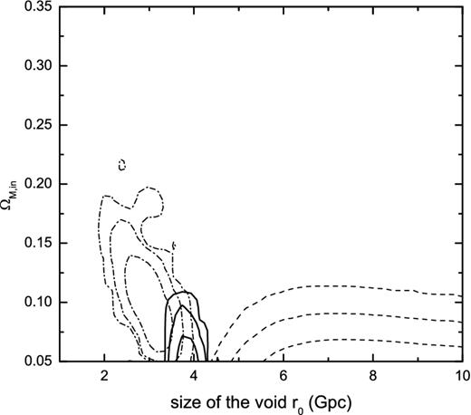
Figure 1.
The 1σ, 2σ and 3σ contours in the parameter space ΩM, in − r0 for the constrained GBH model. The dash–dotted contours represent constraint from SNe Ia+CMB, the dashed contours from AAP and the solid contours from SNe Ia+CMB+AAP. The best-fitting parameters are r0 = 3.0 Gpc and ΩM, in = 0.10 for SNe Ia+CMB. But in order to fit the AAP, much more larger and underdense void are needed. This void model cannot fit both the SNe Ia plus CMB data and the orientations of galaxy pairs.
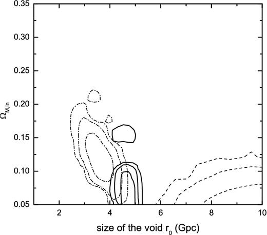
Figure 2.
Same as Fig. 2, but for the Gaussian LTB model. The best-fitting parameters are r0 = 3.6 Gpc and ΩM, in = 0.12 from SNe Ia+CMB. The AAP favours a much more larger and underdense void.
In Fig. 3, we show the theoretical redshift scaling of the AAP in these two LTB models. In the upper panel, we use the best-fitting parameters from SNe Ia+CMB for the constrained GBH model, r0 = 3.0 Gpc and ΩM, in = 0.10. Obviously, the predicted values of AAP deviate from the observational values at high redshift. The χ2 value is 37.35 for these nine data points. In the bottom panel, r0 = 3.6 Gpc and ΩM, in = 0.12 are used for the Gaussian LTB model. The χ2 value is 41.96 for these nine data points.
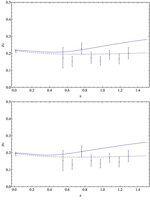
Figure 3.
Points represent the observed AAP. The solid lines represent the theoretical redshift scaling of the AAP as predicted by equation (13) in different LTB models with best-fitting parameters from SNe Ia+CMB, upper panel for constrained GBH and bottom panel for Gaussian LTB. The dashed line shows the best-fitting ΛCDM model with ΩM = 0.25 and |$\Omega _\Lambda$|=0.65.
We must note that the local Hubble constant
Hloc is also a big obstacle to the void models. Because the measurement of the Hubble constant is carried out mostly within a distance of roughly
rloc ∼ 200 Mpc (Riess et al.
2011; Freedman et al.
2012), we obtain (Marra & Paakkonen
2010)
In order to fit both the SNe Ia and CMB, the value of
Hloc is 64 ± 3.2 km s
−1 Mpc
−1 in the constrained GBH model or 63 ± 3.5 km s
−1 Mpc
−1 in the Gaussian LTB model. Riess et al. (
2011) determined the Hubble constant with 3 per cent uncertainty as 73.8 ± 2.4 km s
−1 Mpc
−1. Freedman et al. (
2012) measured the Hubble constant as 74.3 ± 2.1 km s
−1 Mpc
−1.
DISCUSSIONS
Previous investigations show that void models can fit a variety of cosmological observations without containing dark energy because the lack of homogeneity gives a great degree of flexibility. For example, since the last scattering surface is far away from regions where SNe Ia are observed, the property of inhomogeneity allows a model to be constructed which provides different physical densities in the regions from which these two sets of observational data are drawn. So, the best way to constrain inhomogeneous models is using several sets of data that measure a range of observables at comparable redshifts. In this paper, we confront two general classes of void models with observations of SNe Ia, CMB and orientations of galaxy pairs. The redshifts of SNe Ia and orientations of galaxy pairs are almost in the same range. We find that the these two void profiles cannot fit both SNe Ia plus CMB data and orientations of galaxy pairs simultaneously. We also show that the two void models can fit both SNe Ia and CMB data, but at the expense of a Hubble constant so low that they can also be ruled out. So our results favour the Copernician principle. We must also note that our results are obtained under some assumptions, such as the chosen priors and void profile, which is also discussed in Biswas et al. (2010). So the void models are ruled out at the 4σ confidence level given the explored models and priors. But observations challenge the void models (Biswas et al. 2010; Zibin & Moss 2011). Future galaxy surveys such as BigBOSS (Schlegel et al. 2011) will provide the improved precision of the AAP function, placing much more strong constraints on inhomogeneity.
We thank an anonymous referee for helpful comments and suggestions. We have benefited from reading the publicly available code of Marra & Paakkonen (2010). This work is supported by the National Natural Science Foundation of China (grants 11103007 and 11033002).
REFERENCES
et al. ,
ApJS
,
2009
, vol.
182
pg.
543
,
Nat
,
1979
, vol.
281
pg.
358
,
Phys. Rev. D
,
2006
, vol.
74
pg.
103520
et al. ,
ApJ
,
2010
, vol.
716
pg.
712
,
Phys. Rev. D
,
2012
, vol.
86
pg.
A023530
,
J. Cosmol. Astropart. Phys.
,
2010
, vol.
11
pg.
030
,
MNRAS
,
1947
, vol.
107
pg.
410
,
Phys. Rev. D
,
2012
, vol.
85
pg.
103512
,
Phys. Rev. Lett.
,
2008
, vol.
100
pg.
191302
,
J. Cosmol. Astropart. Phys.
,
2011
, vol.
02
pg.
013
,
Phys. Rev. Lett.
,
2008
, vol.
101
pg.
011301
,
Phys. Rev. Lett.
,
2008
, vol.
101
pg.
131302
,
ApJ
,
2006
, vol.
644
pg.
671
,
ApJ
,
2004
, vol.
612
pg.
L101
et al. ,
ApJ
,
2007
, vol.
660
pg.
1
,
MNRAS
,
2002
, vol.
330
pg.
965
et al. ,
ApJ
,
2005
, vol.
633
pg.
560
,
MNRAS
,
2010
, vol.
405
pg.
2231
,
ApJ
,
2012
, vol.
758
pg.
24
et al. ,
A&A
,
2008
, vol.
479
pg.
9
,
J. Cosmol. Astropart. Phys.
,
2008
, vol.
04
pg.
003
,
J. Cosmol. Astropart. Phys.
,
2009
, vol.
09
pg.
028
,
Phys. Rev. D
,
1995
, vol.
52
pg.
1821
et al. ,
Nat
,
2008
, vol.
451
pg.
541
,
ApJ
,
2001
, vol.
549
pg.
669
et al. ,
ApJS
,
2011
, vol.
192
pg.
14
,
MNRAS
,
2012
, vol.
420
pg.
1079
et al. ,
ApJS
,
2011
, vol.
192
pg.
18
,
Ann. Soc. Sci. Brux.
,
1933
, vol.
A53
pg.
51
,
Nat
,
2010
, vol.
468
pg.
539
,
J. Cosmol. Astropart. Phys.
,
2012
, vol.
10
pg.
036
,
J. Cosmol. Astropart. Phys.
,
2010
, vol.
12
pg.
021
,
Phys. Rev. D
,
2011
, vol.
83
pg.
063506
et al. ,
ApJ
,
1999
, vol.
517
pg.
565
et al. ,
AJ
,
1998
, vol.
116
pg.
1009
et al. ,
ApJ
,
2011
, vol.
730
pg.
119
et al. ,
A&A
,
2010
, vol.
516
pg.
A63
et al. ,
Phys. Rev. Lett.
,
2011
, vol.
107
pg.
021302
,
A&A
,
1977
, vol.
59
pg.
53
et al. ,
ApJ
,
2004
, vol.
606
pg.
702
,
Proc. Natl. Acad. Sci. USA
,
1934
, vol.
20
pg.
169
,
Phys. Rev. Lett.
,
2008
, vol.
100
pg.
191303
,
ApJ
,
2012
, vol.
748
pg.
111
,
ApJ
,
2007
, vol.
667
pg.
1
,
MNRAS
,
2011
, vol.
415
pg.
3423
,
Phys. Rev. Lett.
,
2011
, vol.
107
pg.
041301
,
Phys. Rev. Lett.
,
2008
, vol.
78
pg.
043504
,
Class. Quantum Gravity
,
2011
, vol.
28
pg.
164005
,
Phys. Rev. Lett.
,
2008
, vol.
101
pg.
251303
© 2013 The Authors Published by Oxford University Press on behalf of the Royal Astronomical Society


