


Abstract
KIC 8677585 is a roAp star in the Kepler field which is unique in that there are four low-frequency variations of unknown origin in addition to more than 20 high-frequency roAp modes. We analysed all available spectroscopy and conclude that the star has a constant radial velocity and most likely not a binary. We estimate its effective temperature to be Teff = 7300 ± 200 K from high-dispersion spectra. We present an analysis of 829 d of Kepler short-cadence data which shows clear frequency and amplitude variations with a time-scale of months. The dominant low-frequency peak at 3.142 d−1 has the same frequency and amplitude variation as one of the roAp modes. We therefore conclude that the low frequencies are oscillations in the roAp star itself, but the driving mechanism is unknown. We find several frequency spacings among the roAp modes equal to the dominant low frequency, suggestive of non-linear interactions. There is also a clear spacing of 37.2 μHz which we interpret as the large separation and deduce that log g = 3.90 ± 0.03. Models with these parameters which take into account the effect of the magnetic field on the oscillations are able to reproduce the observed range of roAp frequencies, but not the observed large separation. It is found that the properties of the oscillations are sensitive to the assumed stellar parameters and that a more detailed analysis is required. The fact that low frequencies are closely coupled to the roAp frequencies calls into question our current understanding of pulsation in these stars.
INTRODUCTION
Ap stars are A-type stars in which diffusion of elements in a strong magnetic field has led to patches of different abundances and a very large overabundance of rare earth elements. The roAp stars are Ap stars belonging to the SrCrEu group which pulsate with multiple periods in the range 5–20 min. These oscillations are interpreted as magnetoacoustic modes of low spherical harmonic degree (l ≲ 4) and high radial order (typically n ≳ 15). The cause of the pulsation is not known, but could be due to the κ mechanism acting in the region of partial hydrogen ionization. Under normal conditions damping is just larger than driving and the star is stable. By postulating a small temperature inversion in the atmosphere, Gautschy, Saio & Harzenmoser (1998) showed that pulsations in the roAp frequency range could be driven. However, there is no reason for the temperature inversion to be present. At the magnetic poles of roAp stars, the strong vertical magnetic field is thought to suppress convection and enables the oscillations to be driven (Balmforth et al. 2001; Cunha 2002; Saio 2005; Théado et al. 2009).
While this seems a promising model, it does not explain pulsational driving in the cooler roAp stars. For example, Saio, Ryabchikova & Sachkov (2010) find that all roAp-like pulsations are stable in magnetic models of HD 24712 (HR 1217; DO Eri) in which convection is suppressed. A second puzzling aspect is that apparently non-oscillating Ap stars called ‘noAp stars’ occupy a similar part of the HR diagram as the roAp stars. At present it is not clear what determines which of these peculiar magnetic stars show high radial overtone p-mode pulsation, and which are apparently non-variable. This may either be the result of a selective driving mechanism or simply an observational bias.
The global magnetic field which is present in all Ap stars plays an essential role in roAp oscillations, influencing their geometry, frequencies and energy balance. The presence in some roAp stars of frequency multiplets with spacings exactly equal to the frequency of rotation led Kurtz (1982) to introduce the oblique pulsator model, according to which the observed pulsations are axisymmetric about the magnetic axis, which is tilted with respect to the rotational axis. Most roAp stars do not show the rotational multiplets, either because the rotational period is too long (and the multiplets unresolved) or because they have amplitudes below the threshold of detectability. In those stars where rotational multiplets are seen, the spherical harmonic degree of the pulsation, l, may be inferred from the number and relative amplitudes of the multiplets.
In some roAp stars, a pattern of nearly equally spaced frequencies is observed which is unrelated to oblique pulsation. These could be interpreted as consecutive radial overtones, n, of modes with a given l which are approximately equally spaced in frequency in accordance with the asymptotic relation derived by Tassoul (1980). The average spacing is called the large separation, from which the mean density of the star can be determined. In practice, the presence of a magnetic field breaks the spherical symmetry of the pulsating star and perturbs the oscillation frequencies away from the values predicted by the asymptotic relation. This has been shown theoretically in a number of studies that considered oscillations in the presence of a large-scale magnetic field (Cunha & Gough 2000; Saio & Gautschy 2004; Saio 2005; Cunha 2006). According to these works, a pattern of nearly equally spaced peaks may still be found in particular sections of the frequency spectrum, but it is also clear that the magnetic field can distort the regular frequency pattern. This problem can be resolved by matching the observed frequencies with frequencies calculated from models which include the effect of a magnetic field (Saio 2005).
Time-resolved spectroscopy of roAp stars shows a complex picture of propagating magnetoacoustic pulsation waves with amplitudes and phases which vary as a function of atmospheric height. Magnetohydrodynamical simulations of waves in a cool Ap star with a modified atmospheric structure containing a density inversion at the photospheric base are able to reproduce these features (Khomenko & Kochukhov 2009). It seems that the overall height dependence of the pulsations in roAp atmospheres is strongly influenced by the density inversion which seems to be caused by hydrogen ionization. More recently, Sousa & Cunha (2011) obtained approximate analytical solutions for the displacement components of the pulsation in the outermost layers which includes effects of the magnetic field. It is shown that running waves, evanescent waves and standing waves all contribute to the observed radial velocity. A number of case studies are discussed which illustrate the origin of various observational features. While the pulsation amplitude is generally found to increase with atmospheric height, the phase shows a diversity of behaviour. Observations of the oscillation amplitudes with height inferred from spectroscopy have indicated the presence of nodes in the atmosphere. However, Sousa & Cunha (2011) show that these may be false nodes caused by the limited height resolution of the observations.
It is clear that we are far from understanding pulsations in roAp stars, even though impressive advances have been made both observationally and theoretically over the last few years. Scope for further progress has been greatly expanded thanks to high-precision photometry from recent space missions, particularly the Kepler mission. Kepler is designed to detect Earth-like planets around solar-type stars (Koch et al. 2010). To achieve that goal, micromagnitude photometry of over 150 000 stars has been obtained over several years. There are three known roAp stars in the Kepler field: KIC 8677585 (Balona et al. 2011a), KIC 10483436 (Balona et al. 2011b) and KIC 10195926 (Kurtz et al. 2011). The varied properties of roAp pulsations present a wide range of interesting challenges. Each roAp star seems to have its own peculiar characteristics and the three Kepler roAp stars are good examples.
KIC 8677585 does not show rotational multiplets, but shows an unexpected low frequency which is unique and difficult to understand. KIC 10483436 shows a rotational light curve with period Prot = 4.303 d and eight roAp frequencies which are accompanied by multiplets in accordance with the oblique pulsator model. KIC 10195926 shows two pulsation modes with periods that are amongst the longest known for roAp stars at 17.1 and 18.1 min. It also seems to have a low frequency which is nearly half the rotation frequency (Prot = 5.6846 d). Also, it seems that there is more than one oblique axis of pulsation. Finally, there is a forth star, KIC 4840675 which is not an Ap star but shows three high-frequencies characteristic of roAp pulsations (Balona et al. 2012). This may perhaps be due to a pulsating white dwarf in the system.
In this paper, we investigate the pulsations in KIC 8677585. In the analysis by Balona et al. (2011a), only data from the commissioning phase was used consisting of short-cadence (SC) data (1 min exposures) over a 9.73 d period. Since that time, the Kepler data for this star has been accumulating and the possibility exists that new clues to the origin of the roAp pulsations may be obtained by an analysis of the new data. The star is of special interest because the low-frequency variation cannot be understood in the context of pulsational driving by the opacity mechanism. Attempts to understand this frequency include contamination of the photometry by another star (assumed to be the real source of the low frequency) or attributing the low frequency to a γ Doradus pulsation driven by the convective-blocking mechanism. In this paper, we show that neither of these explanations are valid and that the low frequency is, in fact, intimately related to the high-frequency roAp pulsations in a way which is not understood.
SPECTROSCOPY
Ground-based observations are an essential component in the interpretation of Kepler data (Uytterhoeven et al. 2010), and KIC 8677585 is no exception. A few high-resolution spectra of KIC 8677585 have been obtained. An analysis of the spectrum obtained using the HERMES spectrograph on the 1.2-m Mercator telescope at the Roque de los Muchachos Observatory on La Palma, Canary Islands has been described in Balona et al. (2011a). This results in Teff = 7600 ± 200 K, log g = 4.0 ± 0.3, vsin i = 4.2 ± 0.5 km s−1 and a magnetic field modulus of 〈B〉 = 3.2 ± 0.2 kG.
It should be noted that we are dealing with an Ap star. There is no reason why the atmospheric structure in such a star should be the same as the atmospheric structure of a normal main-sequence star. We know that there are abundance patches and vertical stratification and this is bound to change the atmospheric structure. Therefore, the use of a normal stellar atmosphere to describe the Balmer line profiles in an Ap star is only an approximation and one might expect considerable uncertainties in the derived parameters. However, it is certainly true the Balmer line fitting is probably the best method of estimating the effective temperature since the photometric indices are severely compromised by the additional line blanketing caused by the rare earth lines in the spectrum.
An example of the problems faced with fitting Balmer line profiles in cool Ap stars is the ‘core-wing anomaly’ (Cowley et al. 2001). This is most clearly visible in Hα and consists of an unusually narrow and deep core in the line profile. This feature has been a puzzle for many years and is a clear indication of an abnormal atmospheric structure. An attempt has been made to invert the problem and to calculate what atmospheric structure is required to reproduce the sharp Balmer line cores. Kochukhov, Bagnulo & Barklem (2002) find that it is possible to obtain a very good fit by increasing the temperature by 500–1000 K at intermediate atmospheric layers. While making this modification improves the fit, it is not clear whether the resulting stellar parameters are any closer to the true values.
We re-examined the HERMES spectrum and several other spectra of KIC 8677585. Five spectra of KIC 8677585 were acquired at different epochs in 2009 December with the Sandiford Cassegrain Echelle Spectrometer (SES; McCarthy et al. 1993), attached at the 2.1-m (82 arcsec) Otto Struve Telescope of McDonald Observatory (Texas). We used the 1 arcsec slit width, which yields a resolving power of R = 47 000, and set the grating angle to encompass the spectral region 5000–6000 Å. Exposure times were 1800–2400 s. Radial velocities were calculated by multi-order cross-correlation with the radial velocity standard star HD 50692 (Udry, Mayor & Queloz 1999). The error is about 0.28 km s−1 per spectrum, which includes the order-by-order scatter, as well as the long-term stability of the zero-point velocity, which is the dominant error source.
Three spectra were taken on 2010 August 2 (JD 245 5410.90) with the CS23 spectrograph attached to the 2.7-m Harlan J. Smith Telescope of the McDonald Observatory, Texas, USA. Exposure times were 1200–1500 s and the resolution R = 60 000. Radial velocities of these spectra and the HERMES spectrum were obtained by cross-correlating in the wavelength range 4000–5600 Å with a synthetic spectrum with Teff = 7250 K, log g = 4.0 and solar metallicity. Radial velocities are shown in Table 1. The mean radial velocity is Vr = 11.15 ± 0.11 km s−1 from nine spectra (standard deviation 0.33 km s−1). The star clearly has a constant radial velocity and is unlikely to be part of a binary system. Of course, one cannot rule out a binary with a large separation and long orbital period.
Heliocentric radial velocities of KIC 8677585 from high-resolution spectra.
| Spectrum | HJD | Vr |
|---|---|---|
| (245 5000.0+) | (km s−1) | |
| SES | 175.562 | +11.84 |
| SES | 176.571 | +11.48 |
| SES | 177.566 | +10.92 |
| SES | 178.564 | +11.35 |
| SES | 179.572 | +10.89 |
| HERMES | 240.720 | +10.93 |
| CS23 | 410.893 | +11.08 |
| CS23 | 410.910 | +11.00 |
| CS23 | 410.927 | +10.89 |
In the CS23 spectra, only the Hβ line can be used since Hα is only partly observed. We used synthetic spectra calculated from the spectrum code (Gray 2010) using model atmospheres of solar composition and microturbulent velocities of 2 km s−1 by Castelli & Kurucz (2003). We estimated the continuum in these spectra and in the SES spectra by comparing the observed spectrum with a range of synthetic spectra covering a suitable range in effective temperature and surface gravity. The line profile of Hβ obtained in this way agrees almost exactly with the HERMES line profile in all spectra. Since the continuum in the HERMES spectra was estimated independently in an entirely different manner, we are confident that the error in the continuum placing is small.
By comparing the observed and synthetic line profiles in Hα and Hβ, it is clear that there is a core-wing anomaly in this star. We found that the sharp core can only be matched using cooler models as found by Cowley et al. (2001). We are thus faced with a problem of whether to use the core only, the wings only or some intermediate fit.
Fig. 1 shows a grid of model fits of the Hβ line. The core is fitted quite well with Teff = 7000 K, log g = 5.0, but the wings are better fitted with Teff = 7250 K. The fit of the wings is not very sensitive to log g. For higher temperatures, the fit to the core is very poor and the wings are too broad. The best compromise is probably Teff = 7250 K, log g = 4.0, but there is clearly a rather large uncertainty in Teff. Note that the observed spectrum contains many metal lines which are not matched by the synthetic spectrum. These are, of course, lines of rare earth elements due to the Ap nature of the star. It is the overall profile of the Hβ line which determines Teff and the best was estimated by eye rather than a least-squares fit which requires all metal lines to be either removed or properly modelled.
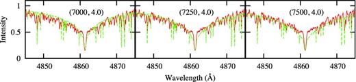
Observed Hβ line profile (red solid curve) and synthetic profiles (green dashed curve) for various values of (Teff, log g).
We have already mentioned that the atmospheric structure of Ap stars must differ from that of normal Ap stars (Kochukhov et al. 2002) to account for the core-wing anomaly. It has also been shown that in Ap stars with dipolar magnetic fields above 1–2 kG, the Balmer line profiles are modified by several percent due to the effect of the Lorentz force (Stepien 1978; Valyavin, Kochukhov & Piskunov 2004; Shulyak et al. 2007). Since the magnetic field modulus of KIC 8677585 is above this range, it is reasonable to expect deviations in the Balmer line profiles relative to those in a non-magnetic star with the same physical parameters. Our overall conclusion is that we cannot determine the effective temperature with the precision expected for a normal star. Estimating Teff from the photometry is, of course, equally problematic since we do not know the effect of line blanketing. The best we can do is to compare the fit of the Balmer line wings with synthetic spectra, from which we estimate Teff = 7300 ± 200 K and log g = 4.0 ± 0.5.
Kepler PHOTOMETRY
For the vast majority of stars, Kepler photometry is available only in long-cadence (LC) mode which consist of practically uninterrupted 30-min exposures. KIC 8677585 has also been observed in SC mode (1-min exposures). It is possible to extract frequencies beyond the Nyquist frequency of LC data because the sampling interval is not exact (Murphy, Shibahashi & Kurtz 2013), but a direct comparison between LC and SC data of KIC 8677585 shows that the roAp frequencies, which are at least five times higher than the Nyquist frequency, are not reliably extracted in the LC data. For frequencies higher than about 24 d−1, only SC data were used. Characteristics of SC data are described in Gilliland et al. (2010), while Jenkins et al. (2010b) describe the characteristics of LC data. The science processing pipeline is described by Jenkins et al. (2010a). Following each quarter of a 370-d Kepler solar orbit, there is a pause while data from Kepler are downloaded. The Kepler data are therefore divided according to the approximately 90-d quarters which are numbered Q0, Q1, Q2, etc. (Q0 being the initial 10-d commissioning run).
For KIC 8677585, LC data are available for Q0–Q13 which consists of almost continuous 30-min exposures over a time span of 1152 d. The SC data consist of Q0, covering 9.73 d from BJD 245 4953.54–245 4963.24, and Q5–Q13, covering 829.58 d from BJD 245 5276.49–245 6106.05. The latter are almost continuous 1-min exposures except for a break of 16 d between Q7 and Q8 and smaller breaks of about one day between the other quarters. There are 14 238 observations in Q0 and 1146 612 observations in Q5–Q13.
The light-curve files contain simple aperture photometry (SAP) flux and a more processed version of SAP with artefact mitigation included called pre-search data conditioning (PDC) flux. Significant systematic and stochastic errors occur in the SAP photometry which include discontinuities, outliers, systematic trends and other instrumental signatures. The PDC tries to remove these errors while preserving astrophysically interesting signals. This makes use of a subset of highly correlated and quiet stars to generate a cotrending basis vector set which is in turn used to establish a range of reasonable robust fit parameters. The PDC flux uses the best fit that simultaneously removes systematic effects while reducing the signal distortion and noise injection. Details of how this is accomplished are described in Stumpe et al. (2012) and Smith et al. (2012).
Visual inspection of the PDC light curves shows, however, that clear instrumental trends are still visible. As a result we decided not to use the PDC data, but rather the original raw data which were corrected by hand. The process involves removing clear outliers and fitting individual quarters by low-order polynomials to remove long-term trends. Finally, jumps between quarters were eliminated by adjusting the data to ensure smooth continuation. As a result of these corrections, we expect to lose information for frequencies less than about 0.1 d−1.
FREQUENCY ANALYSIS
Due to the long gap between Q0 and Q5 which might introduce an unnecessary alias pattern, we decided to use only the Q5–Q13 SC data for frequency extraction. After removal of outliers and data correction there are 1126 936 data points in this set. The frequency analysis was carried out using a fortran code based on the fast computation of the Lomb periodogram (Lomb 1976) using the algorithm of Press & Rybicki (1989). The frequency of highest amplitude is assumed to be the correct frequency and is added to the list of extracted frequencies. The original data are fitted to a multiperiodic Fourier series containing all extracted frequencies and the frequency search is continued using the residuals (pre-whitened data). A maximum of 50 simultaneous frequencies are used for the Fourier fit. When this limit is reached, the data pre-whitened by the 50 frequencies are treated as the original data and the process is continued.
The data are almost equally spaced, so one could make use of the fast Fourier transform (FFT) by mapping the data on to an exactly equally spaced grid. The mapping was done by simple linear interpolation between neighbouring points using a time interval of 58.85 s. The resulting FFT is practically identical to the Lomb periodogram, but the processing time is orders of magnitude smaller.
We begin by computing the periodogram of the whole data set. Periodograms in various frequency ranges are shown in Fig. 2. For the low-frequency range, it is possible to use the LC data which cover Q0–Q13. The resulting periodogram is shown in the bottom panel of Fig. 2. The ranges of interest can be divided into three frequency groups: low frequency (2–7 d−1), middle frequency (1480–1690 μHz) and high frequency (3160–3330 μHz). There are no significant peaks outside these regions.
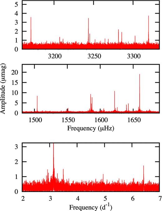
Periodograms of the Q5–Q13 from the SC combined data (top two panels). The bottom panel is from the Q0–Q13 LC data.
It is apparent that the peaks in Fig. 2 are not single but contain structure. Fig. 3 shows the details around the most prominent peaks as well as the window function. From the window function it is clear that some non-stationary process is in action. The appropriate tool for examining non-stationary processes in a time series is a time–frequency diagram. To construct such a diagram, we calculate the periodogram at a particular time. This involves a choice of the length of the time series that is to be used. If it is too short, one obtains good time resolution but poor frequency resolution. By trial and error, we found that a time series of length 178.55 d (N = 218 data points) was a good compromise. The FFT of a time series of length N results in N/2 independent Fourier frequencies and phases which fully describes the data. We interpolated the power between the Fourier frequencies by the simple expedient of padding the data with zeros for a total length of 220 data points at each time step.
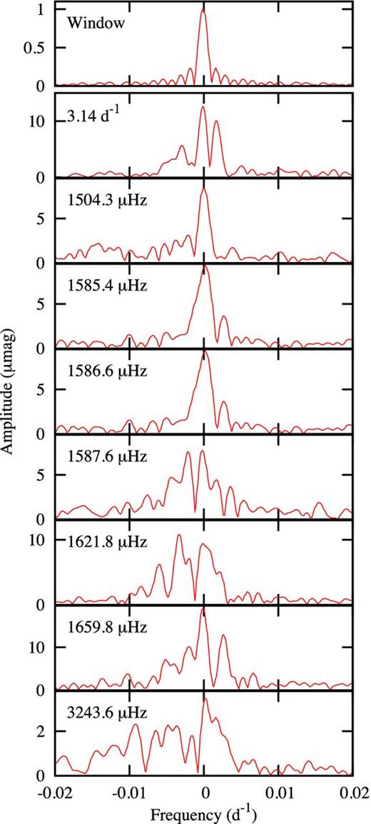
Details around individual peaks of Fig. 2.
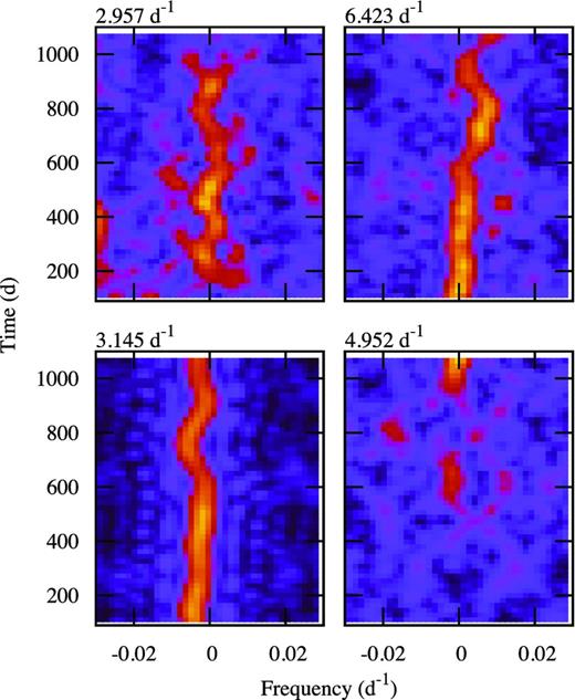
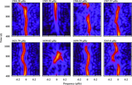
It is apparent that all modes vary in frequency and amplitude. In Fig. 4, we show the amplitude variation as a function of time for some of the peaks of highest amplitude. Fig. 5 shows the time–frequency diagrams for the same peaks. The fine structure of the peaks shown in Fig. 3 are evidently due to substantial frequency and amplitude variations with a time-scale of months. Fig. 6 shows the time–frequency diagrams for the low frequencies where data from Q0–Q15 are available. Note that the frequency and amplitude variation of the 3.142 d−1 mode matches that of the 1621.79 μHz mode and that the frequency variation of the 6.423 d−1 mode matches that of the 1659.8 μHz mode.
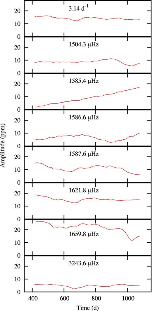
Time–amplitude diagrams for the modes of highest amplitude. The time is relative to JD 245 4950.000.
Time–frequency diagrams for the modes of highest amplitude using SC data. The time is relative to JD 245 4950.000.
Time–frequency diagrams for low-frequency modes using Q0–Q13 LC data.
In Table 2, we list the mean frequencies and amplitudes for all detectable peaks. We notice that some frequencies listed by Balona et al. (2011a) from Q0 are not detected in the Q5–Q13 data. Since the amplitudes of the modes vary quite dramatically, it is possible that some peaks with detectable amplitudes in Q0 might have amplitudes too low to be observed at the later time.
Frequencies and amplitudes for the combined Q5–Q11 data set for KIC 8677585. The first column lists the identification numbers from Balona et al. (2011a). Values in italics are uncertain because of low amplitude and because the modes are not always visible.
| n | ν (d−1) | ν (μHz) | A (μmag) |
|---|---|---|---|
| 9 | 2.957 | 34.22 | 2.5 |
| 3 | 3.142 | 36.37 | 12.0 |
| 4.952 | 57.31 | 1.1 | |
| 6.423 | 74.36 | 1.7 | |
| 10 | 126.01 | 1458.5 | 8.4 |
| 7 | 129.970 | 1504.28 | 10.4 |
| 133.838 | 1549.05 | 2.3 | |
| 134.022 | 1551.18 | 2.7 | |
| 136.62 | 1581.3 | 1.6 | |
| 136.826 | 1583.63 | 2.0 | |
| 136.842 | 1583.82 | 2.9 | |
| 136.978 | 1585.39 | 6.9 | |
| 6 | 137.084 | 1586.62 | 5.3 |
| 4 | 137.166 | 1587.57 | 9.5 |
| 11 | 138.44 | 1602.3 | 8.4 |
| 138.684 | 1605.14 | 1.9 | |
| 138.705 | 1605.38 | 2.6 | |
| 2 | 140.123 | 1621.79 | 13.7 |
| 140.262 | 1623.40 | 2.7 | |
| 140.480 | 1625.93 | 3.1 | |
| 141.680 | 1639.82 | 4.8 | |
| 141.928 | 1642.68 | 3.3 | |
| 143.265 | 1658.16 | 3.0 | |
| 1 | 143.406 | 1659.79 | 21.5 |
| 8 | 144.69 | 1674.7 | 9.1 |
| 5 | 144.81 | 1676.0 | 14.7 |
| 273.956 | 3170.79 | 2.8 | |
| 277.10 | 3207.2 | 1.4 | |
| 277.46 | 3211.4 | 1.2 | |
| 280.246 | 3243.59 | 4.5 | |
| 280.386 | 3245.21 | 1.9 | |
| 283.527 | 3281.56 | 2.8 | |
| 283.886 | 3285.72 | 2.4 | |
| 285.334 | 3302.48 | 1.6 | |
| 286.815 | 3319.62 | 4.5 |
THE LARGE SEPARATION
It turns out that there is a pattern in the frequencies of Table 2. If one calculates all possible frequency differences, the distribution shows a preferred frequency spacing of 19.0 or 37.2 μHz. This pattern is still easily visible if the frequencies are restricted to those in the mid-range, as shown in Fig. 7. In the figure, the peak at 37.2 μHz is higher than the one at 19.0 μHz. We suspect that the smaller spacing is the frequency separation between consecutive l = 0 and l = 1 modes and that the larger spacing corresponds to the large separation, Δν = 37.2 ± 0.6 μHz.
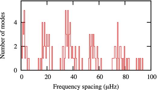
Histogram of frequency spacings in frequencies 1450–1700 μHz.

Location of KIC 8677585 in the theoretical HR diagram with one standard deviation error bars. Other roAp stars (open circles) and noAp stars (small crosses) are also shown. The zero-age main-sequence and evolutionary models of solar composition and indicated masses are from Bertelli et al. (2008).
Fig. 9 shows the echelle diagram for the mid-frequency peaks using Δν = 37.2 μHz. There are two distinct ridges, one of which we could assign to l = 1 modes (left-hand ridge in Fig. 9) and the other to a mixture of l = 0 and l = 2 modes (right-hand ridge). This could, of course, be the other way round. Note that although it is possible to construct an echelle diagram for this star, just as in the case of many stars with solar-like oscillations, the driving of roAp modes occurs by a different mechanism than the stochastic driving in solar-like oscillations. Unlike in solar-like oscillations, a frequency of maximum amplitude, νmax, does not exist.
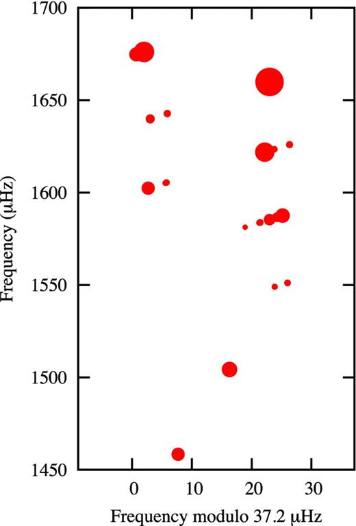
Echelle diagram for the mid-frequency modes using Δν = 37.2 μHz. The size of the symbols are proportional to the mean amplitude of the modes. All modes in Table 2, including uncertain modes, are included.
One problem is why there are so many closely spaced modes on the l = 0, 2 branch (in fact on both branches). The typical spacing between these modes is approximately 5μHz (about 0.5 d−1) which is far too large to be rotational splitting. It is clear that the star is a very slow rotator with a rotation period measured in tens or hundreds of days. If this were not the case, we should see the rotational light curve and also the equally spaced multiplets predicted by the oblique rotator model.
One could presume that these are modes of higher l, but these should have low amplitudes owing to cancellation effects. Indeed, in Kepler observations of solar-like stars modes with l > 2 are difficult to detect. However, in a roAp mode, the horizontal motion can be comparable to the vertical motion, in spite of the high radial order of the pulsations (Saio & Gautschy 2004). The fact that the eigenfunction of the high-frequency modes is so different from a simple spherical harmonic could enhance the visibility of high-degree modes. This may explain the large number of closely spaced modes on the l = 0 and l = 0, 2 ridge lines in the echelle diagram. It is also possible that some of the modes may not be independent modes, but a result of non-linear interaction with the 3.142 d−1 mode (see below).
As already mentioned, a magnetic field introduces frequency shifts, relative to a non-magnetic model, which vary with frequency and magnetic field strength in a cyclic manner with sudden jumps. The damping rate also changes cyclically with respect to the pulsation frequency and strength of the magnetic field (Cunha & Gough 2000; Saio & Gautschy 2004). These frequency shifts significantly affects the large separation, particularly if the frequencies lie on either side of a jump. The energy loss suffered by coupling of the pulsations with the magnetic field also results in a strong selection effect in which modes that are expected to be seen are absent. There are certainly amplitude changes along the ridge lines, as can be seen from the sizes of the symbols in Fig. 9, but these do not seem particularly drastic. The frequency shifts, if they exist, cannot be too large either. The cyclic effects on the frequency could explain, however, why the regular spacing seems to break down at frequencies below about 1550 μHz.
It is also interesting to note that the large-amplitude mysterious low frequency ν3 = 3.142 d−1 (36.37 μHz) is close to Δν, but this could just be coincidence. There is no physical basis to expect a mode at Δν, of course. We also note that the frequency differences among several of the roAp modes are very close to ν3, as shown in Table 3 and Fig. 10. It is possible that some of the low-amplitude modes, such as 1549.05, 1551.18, 1658.16 and 1623.40 μHz might not be independent modes but a result of non-linear interactions with the high-amplitude modes 1585.39, 1587.57, 1621.79 and 1659.79 μHz, respectively. However, both 1585.39 and 1621.79 are of high amplitude and yet they are spaced by 36.40 μHz. One would have thought that if 1585.39 is a result of non-linear interaction of ν3 with 1621.79, it would be of much lower amplitude.
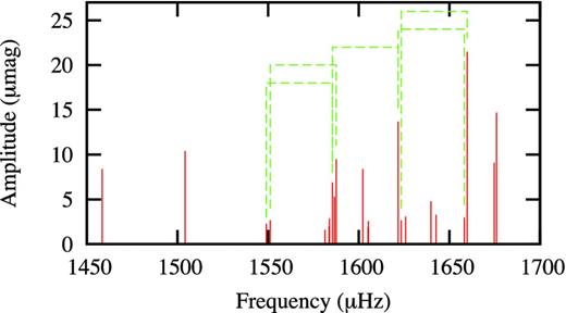
Schematic periodogram of the intermediate-frequency range showing frequency spacings of 3.142 d−1.
Frequency spacings among roAp modes which are close to the dominant low frequency at 36.37 μHz.
| νA | νB | νB − νA |
|---|---|---|
| 1549.05 | 1585.39 | 36.34 |
| 1551.18 | 1587.57 | 36.39 |
| 1585.39 | 1621.79 | 36.40 |
| 1621.79 | 1658.16 | 36.37 |
| 1623.40 | 1659.79 | 36.39 |
| 3170.79 | 3207.20 | 36.39 |
| 3207.20 | 3243.59 | 36.41 |
| 3245.21 | 3281.56 | 36.35 |
| νA | νB | νB − νA |
|---|---|---|
| 1549.05 | 1585.39 | 36.34 |
| 1551.18 | 1587.57 | 36.39 |
| 1585.39 | 1621.79 | 36.40 |
| 1621.79 | 1658.16 | 36.37 |
| 1623.40 | 1659.79 | 36.39 |
| 3170.79 | 3207.20 | 36.39 |
| 3207.20 | 3243.59 | 36.41 |
| 3245.21 | 3281.56 | 36.35 |
MODELING
In modelling the oscillation spectra of roAp stars, it is necessary to include the magnetic perturbation of individual frequencies in a large grid of models. These models need to cover not only the classical parameter space (temperature, gravity, metallicity) and a range of parameters related to convection, convective overshoot and diffusion, but also different magnetic field properties. Such a task is beyond the scope of this paper and shall be addressed in a follow up work. Here, we will only discuss the question of whether modes in the observed frequency range in KIC 8677585 can be driven by the opacity mechanism assuming the global parameters derived in Section 5. To that end, we performed linear, non-adiabatic calculations on stellar models with envelope convection suppressed, using the equilibrium and pulsation codes described in Balmforth et al. (2001) and Cunha (2002). In addition to mass, effective temperature, luminosity and interior chemical composition, these models require the specification of the surface helium abundance and of the boundary condition to be applied to the pulsations at the temperature minimum. For the latter, two options are available: fully reflective or transmissive. In the fully reflective boundary condition, oscillations are reflected regardless of their oscillation frequency. The transmissive boundary condition allows waves with frequencies above the acoustic cutoff frequency to propagate as running waves in the atmosphere.
Fig. 11 shows the relative growth rates obtained for three possible models considered for KIC 8677585, all with mass M = 1.8 M⊙. A positive growth rate means that the corresponding mode is predicted to be excited. The characteristics of these models are presented in Table 4. For all three models, it was assumed that envelope convection is suppressed by the magnetic field and the envelope helium abundance was assumed to be homogeneous. Models A and B were obtained with the reflective outer boundary condition, while model C was obtained with the transmissive boundary condition.
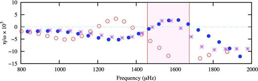
Relative growth rates for the three models described in the text and Table 4, shown as a function of frequency. The relative growth rates are defined by the ratio between the imaginary η, and real, ω, parts of the eigenfrequencies. Open circles – model A; filled circles – model B; asterisks – model C. The shaded area is the range of observed frequencies.
Model, effective temperature, luminosity and type of outer boundary condition applied (see the text for details).
| Boundary | |||
|---|---|---|---|
| Model | Teff (K) | log (L/L⊙) | condition |
| A | 7300 | 1.20 | Reflective |
| B | 7400 | 1.13 | Reflective |
| C | 7300 | 1.10 | Transmissive |
| Boundary | |||
|---|---|---|---|
| Model | Teff (K) | log (L/L⊙) | condition |
| A | 7300 | 1.20 | Reflective |
| B | 7400 | 1.13 | Reflective |
| C | 7300 | 1.10 | Transmissive |
Inspection of Fig. 11 shows that the frequency region in which oscillations are predicted to be excited in the models depends strongly on the assumed global parameters. In model A, the model with effective temperature and luminosity equal to the central values of the intervals given in Section 5, the frequency range of excited modes is well below the observed frequencies (marked by the shaded region). In model B, with a slightly smaller luminosity and slightly higher temperature, but still within the quoted uncertainties, the frequency range of excited modes agrees rather well with the observations. A similar good fit is found with model C, in which a different outer boundary condition was applied.
Despite the apparent success of models B and C in predicting the correct frequency range for the excited modes, we should note that the large separations of models B and C are larger than the value derived in this paper. Thus, only a full analysis of the oscillation spectrum of KIC 8677585, taking into account the direct magnetic effect on the oscillation frequencies, may confirm, or otherwise, refute, these models. It is also interesting to note the strong sensitivity of the results on the assumed global parameters. This fact could be used to derive the global parameters with high precision. We note, also, that models with reduced surface helium abundance predict, for the same global parameters, excited frequencies that are systematically smaller than those predicted by models with homogeneous helium abundance. Models with reduced surface helium abundance are more appropriate when envelope convection is suppressed (Théado, Vauclair & Cunha 2005).
DISCUSSION
KIC 8677585 is the only roAp star in which low frequencies are clearly present. KIC 10195926, another Kepler roAp star, seems to show a low-frequency mode with about half the frequency of rotation and may be another example (Kurtz et al. 2011). In Balona et al. (2011a), it was argued that the 3.142 d−1 frequency cannot be due to rotation or orbital motion. Two explanations were proposed. In one scenario, it is postulated that the origin of the low frequency is not the roAp star, but another star in the same aperture or even a binary companion to the roAp star. Another explanation is that the low frequency is simply a γ Doradus-type pulsation driven by the convective blocking mechanism.
In this paper, we show that the time variation of both the frequency and amplitude of the 3.142 d−1 peak is the same as that of the second-highest amplitude roAp pulsation at 1621.79 μHz. This behaviour clearly implies that the low frequency and the roAp frequencies are related and occur in the same star. Moreover, it does not seem possible to attribute the low frequency to a different driving mechanism because the very different resonant cavities are hardly likely to lead to the same frequency and amplitude variations. The 3.142 d−1 mode corresponds to a g mode with radial order n ≈ 5–10 if l = 1 or n ≈10–20 if l = 2 in a normal main-sequence star with M = 1.8 M⊙. It seems that the mechanism responsible for driving roAp pulsations can also drive intermediate radial order g-mode pulsations in the same star.
Amplitude variations of pulsation modes can always be explained by a change of mode energy, even if we do not understand the mechanism for variation in mode energy. Frequency variations are more difficult to understand. Frequency variations in roAp stars are not unknown. The pulsation frequency of the dominant mode in the roAp star HR 3831 varies with a peak-to-peak amplitude of 0.12 μHz on a time-scale of about 1.6 yr (Kurtz et al. 1994). In a subsequent study (Kurtz et al. 1997), the variation in frequency was confirmed, but it was shown that it cannot be due to Doppler shifts and must be intrinsic to the star. In addition, the pulsation amplitude seems to vary with the frequency. Large amplitude variations with a time-scale of several days have also been seen in the roAp modes of HR 1217 (White et al. 2011).
The variation in frequency must be due to a change in the resonant cavity, but there is no obvious explanation of why such a change should occur. As far as we know, roAp stars are stable over many decades, as can be seen by the precise repeatability of their rotational modulation light curves. These stars are not known to be active, yet something seems to have perturbed KIC 8677585 around JD 245 5650.0, causing a sudden change in frequency in all modes. Perhaps this may be a result of a change in magnetic field strength which could lead to changes in frequency and amplitude owing to the effects already described (Cunha & Gough 2000; Saio & Gautschy 2004). This would be interesting since the magnetic fields in Ap stars are thought to be of fossil origin and there is no particular reason why the magnetic field strength should vary in this way.
Another finding presented here is the distinctive spacing among the modes. We suggest that this is due to consecutive overtones of modes of the same l, from which a large separation Δν ≈ 37.2 μHz is derived. The interpretation of this diagram is complicated by the many closely spaced frequencies in each branch. Because the star rotates very slowly, we do not expect to detect rotational splitting of the modes. We suggest that the multiple frequencies are modes with l > 2 in which the visibility is increased owing to their peculiar eigenfunctions. Alternatively, it is possible that many of the lower amplitude modes might not be real eigenfrequencies but a result of non-linear interaction with the 3.142 d−1 mode. The high sensitivity of the pulsation frequencies to the stellar parameters offers the possibility of determining the stellar parameters with high precision.
It is clear that these observations have opened up a new and unexpected perspective on the nature of roAp pulsations. It seems that we need to search for a way in which g modes can be driven by the same mechanism which drives the high-frequency roAp p modes.
The authors wish to thank the Kepler team for their generosity in allowing the data to be released and for their outstanding efforts which have made these results possible. Funding for the Kepler mission is provided by NASA's Science Mission Directorate.
LAB wishes to thank the South African Astronomical Observatory for and the National Research Foundation for financial support. KU acknowledges financial support by the Spanish National Plan of R&D for 2010, project AYA2010-17803. MC acknowledges financial support from the FCT through the grant SFRH/BPD/84810/2012. This research made use of funds from the ERC through the project FP7-SPACE-2012-312844.
This work is partly based on observations obtained with the HERMES spectrograph, which is supported by the Fund for Scientific Research of Flanders (FWO), Belgium, the Research Council of KU Leuven, Belgium, the Fonds National Recherches Scientific (FNRS), Belgium, the Royal Observatory of Belgium, the Observatoire de Genève, Switzerland and the Thüringer Landessternwarte Tautenburg, Germany.
This paper includes data taken with the 2.1-m Otto Struve telescope and 2.7-m Harlan J. Smith telescope of McDonald Observatory of The University of Texas at Austin, as well as observations made with the Mercator Telescope, operated on the island of La Palma by the Flemish Community, at the Spanish Observatorio del Roque de los Muchachos of the Instituto de Astrofisica de Canarias.
