


Abstract
Extracting stellar fundamental parameters from Spectrointerferometric (SPI) data requires reliable estimates of observables and with robust uncertainties (visibility, triple product, phase closure). A number of fine calibration procedures are necessary throughout the reduction process. Testing departures from centrosymmetry of brightness distributions is a useful complement. Developing a set of automatic routines called spidast (made available to the community) to reduce, calibrate and interpret raw data sets of instantaneous spectrointerferograms at the spectral channel level, we complement (and in some respects improve) the ones contained in the amdlib Data Reduction Software. Our new software spidast is designed to work in an automatic mode, free from subjective choices, while being versatile enough to suit various processing strategies. spidast performs the following automated operations: weighting of non-aberrant SPI data (visibility, triple product), fine spectral calibration (subpixel level), accurate and robust determinations of stellar diameters for calibrator sources (and their uncertainties as well), correction for the degradations of the interferometer response in visibility and triple product, calculation of the centrosymmetry parameter from the calibrated triple product, fit of parametric chromatic models on SPI observables, to extract model parameters. spidast is currently applied to the scientific study of 18 cool giant and supergiant stars, observed with the VLTI/AMBER facility at medium resolution in the K band. Because part of their calibrators have no diameter in the current catalogues, spidast provides new determinations of the angular diameters of all calibrators. Comparison of spidast final calibrated observables with amdlib determinations shows good agreement, under good and poor seeing conditions.
INTRODUCTION
The power of optical–infrared interferometry to obtain information about the astronomical source morphology (including the angular size) is now well established. To properly determine the source properties, the quality of the measurements is an issue, which is still the subject of active research. As with any other measuring apparatus, the absolute calibration of the instrument (including atmosphere) requires careful attention. Derived from the measurement of the mutual degree of coherence of the incident radiation field, on spatial frequencies sampled by the aperture-array configuration, the final interferometric observables are non-linear mixes of noisy quantities, and of parameter estimates with their own uncertainties.
In this paper, we propose to revisit and extend the existing data processing and calibration methods, in the aim to obtain reliable estimates and robust uncertainties for calibrated measurements of visibility and complex triple product. The careful reduction process, described in this paper, has been elaborated for the scientific study of a sample of 18 bright cool giant and supergiant stars (see Table 1). Measurements were obtained with the VLTI/AMBER facility at medium spectral resolution (|${\cal R}$| = 1500) in the K band, using triplets of 1.80-m auxiliary telescopes. Observations have been conducted during 15 observing nights between 2009 May and 2010 December (under Belgian VISA Guaranteed Time). The aim of this work is to test the data reduction and calibration software, on data with various qualities, that we started to develop in 2006.
DEFINING THE BASIC INTERFEROMETRIC OBSERVABLES
The coherent fluxcij is provided by the measurement of the instantaneous observables delivered by the AMBER data reduction software amdlib.1 This quantity traces the sine-like modulated component superimposed on the continuum component, in the observed intensity distribution. It is computed using a χ2 linear fit of the individual interferograms in the detector plane, for each spectral channel (see Tatulli et al. 2007 for details).
At this point, we define the other interferometric observables:
- the squared flux, which is the product of the photometric fluxes pi and pj, associated with the baseline |$\boldsymbol {B}_{ij}$|(1)\begin{equation} f^{2}_{ij} = p_{i} p_{j}; \end{equation}
- the squared visibility, which is the ratio of the squared modulus of the coherent flux to the squared flux(2)\begin{equation} v^{2}_{ij} = \frac{\left| c_{ij} \right|^{2}}{f^{2}_{ij}}; \end{equation}
- the complex bispectrum (Weigelt 1977), which is the product of the three coherent fluxes contributing to the baseline triplet |$\left(\boldsymbol {B}_{12}, \boldsymbol {B}_{23}, \boldsymbol {B}_{31}\right)$|(3)\begin{equation} b_{123} = c_{12}c_{23}c_{31}; \end{equation}
- the triple product, which is the ratio of the bispectrum to the product of the three fluxes contributing to the baseline triplet(4)\begin{equation} t_{123} = \frac{b_{123}}{f_{12}f_{23}f_{31}}; {\rm and} \end{equation}
- the closure phase, which is the argument of the complex bispectrum (or triple product)(5)\begin{equation} \psi _{123} = \arg b_{123} = \arg t_{123}. \end{equation}
REDUCING THE RAW DATA
To process the temporal series of frames (composing the ‘exposures’) produced by the AMBER instrument, we use the data reduction software amdlib, which consists of a core library of C functions plus a high-level interface in the form of a Yorick2 plugin (a high-level language environment, similar to idl or matlab, which is in the public domain).
The standard procedure to extract the basic interferometric observables from the AMBER raw data includes a frame-selection step, which provides a set of ‘good’ frames according to a given criterion, or a sequence of several selection criteria (Malbet et al. 2011). The criterion used the most is based on the signal-to-noise ratio (SNR) of the fringe contrast in each frame. Two selection methods are provided in standard by amdlib:
retaining a given percentage of frames sorted according to their SNR values (called the ‘percentage’ method) and
retaining the frames with SNR values higher than a given threshold (called the ‘threshold’ method).
With both methods, the choice of the optimal value (assumed not biasing the final results) of the selection criterion (in percentage of threshold) is done a posteriori from a sequence of processings using different values of the selection criterion (see Millour et al. 2007 for details). Two drawbacks of this are: the need for a several steps procedure (to be performed manually) and the risk for biasing the final results if the selection criterion is ill determined.
In our method, that we have implemented in a specific Yorick script added to amdlib, we apply the automatic procedure:
remove only the aberrant measurements (in squared visibility and triple product), for each spectral channel independently. Using this specific script results in amounts of useful data larger than the amount obtained with the standard procedure, without increasing biasing effect (only the lower and upper tails of the input data histograms are rejected);
assign a weight to each individual measurement. After many preliminary tests, we decided to choose weights based on the SNR of the coherent flux and on the piston deviation; and
compute the temporal weighted average of the squared visibility and triple product for each spectral channel, with uncertainties derived from the bootstrap technique invented by Efron (1979).
These automatic operations mentioned above, needing neither several step selection nor manual choice of the optimal value of the selection criterion, are described in more details in the following subsections.
Rejecting the aberrant data
To remove the aberrant measurements, we use a combination of physical and statistical basic criteria:
strictly positive sum and product of the fluxes in the photometric channels, since negative flux measurements result from shortcomings in the determination of the continuum in each spectrum;
coherent-flux SNR higher than unity, since inclusion of data with low-SNR values reduces the reliability of the estimators of the interferometric observables (Millour et al. 2008); and
squared visibility greater than Q1 − 1.5 × IQR and lower than Q3 + 1.5 × IQR (‘box-plot filtering’), where Q1 denotes the first quartile, Q3 the third quartile and IQR = (Q3 − Q1) the interquartile range (Hoaglin, Mosteller & Tukey 1983). With triple product data, this third criterion applies to the squared visibility for each baseline, and box-plot filtering on tan ψ123 is added to the list of criteria.
Based on the removal of aberrant measurements at the spectral channel level, rather than on the selection of the ‘best’ frames, our approach provides an amount of useful data larger than the amount obtained with the standard frame-selection procedure. For data shown in Fig. 1, obtained for a ‘good’ seeing on the calibrator target γ Lib, the number of removed input data varies only slightly from one spectral channel to the other (typically less than 3 per cent). Besides, various amount of data are rejected, according to the seeing conditions.
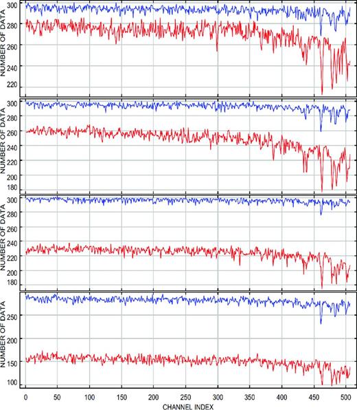
Spectral distribution (in K) of the number of non-aberrant data, remaining after box-plot filtering, from an exposure of 300 input frames with the calibrator γ Lib. From top to bottom: baselines A0–D0 (32 m), D0–H0 (64 m), A0–H0 (96 m) and triplet A0–D0–H0. Blue lines: good seeing conditions (seeing angle = 0.5 arcsec, coherence time = 13 ms). Red lines: poor seeing (1.7 arcsec, 1.3 ms).
Using the seeing parameters ε0 (seeing angle) and τ0 (coherence time), the percentages of rejected data, respective to three baselines and two seeing conditions are given in the following lines (where ‘good seeing’ refers to ε0 = 0.5 arcsec, τ0 = 13 ms, and ‘poor seeing’ refers to ε0 = 1.7 arcsec, τ0 = 1.3 ms):
shortest baseline A0–D0 (32 m): 2 per cent (good seeing) to 9 per cent (poor seeing);
intermediate baseline D0–H0 (64 m): 2 per cent to 16 per cent;
longest baseline A0–H0 (96 m): 2 per cent to 25 per cent; and
in addition, for the baseline triplet A0–D0–H0, the rejection of data amounts 7 and 50 per cent.
Fig. 2 shows the variation of the final squared visibility (at 2.2 μm) produced with amdlib, w.r.t. the percentage of selected frames, based on the SNR and pertaining to the calibrator target γ Lib, observed with the shortest baseline A0–D0 (32 m) in good- and poor seeing conditions (top panel and bottom panel, respectively). The squared visibility produced with our method is shown for comparison.
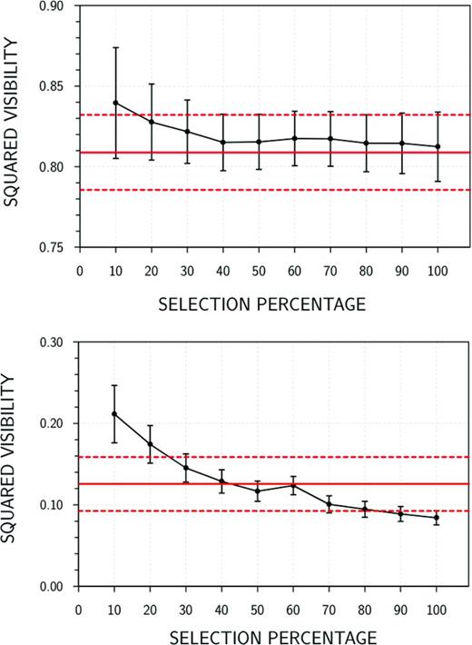
Squared visibility at 2.2 μm obtained with amdlib (black solid lines + error bars) w.r.t. the percentage of selected frames sorted according to their SNR value, for the calibrator γ Lib (baseline A0–D0). Top panel: good seeing conditions. Bottom panel: bad seeing. Red lines: values obtained with our method (solid line: central value; dashed lines: upper and lower limits given by the associated uncertainty).
In this example, the position of the plateau of each curve indicates a value of the selection threshold of 50 per cent, giving the a posteriori determination with amdlib. There we find that our automatic method gives a squared-visibility value close to the 50 per cent value, without a need for the several steps procedure, in good and poor seeing conditions. Besides, Fig. 3 shows that the standard amdlib frame-selection method keeps the extremal V2 values in poor seeing condition, which may bias the result of the calculation of the average over the frames contained in each exposure. On the contrary, the box-plot filtering used with our method rejects only the lower and upper tails of the V2 histogram, thus, leading to estimates of the temporal average, more reliable than with the frame-selection method.
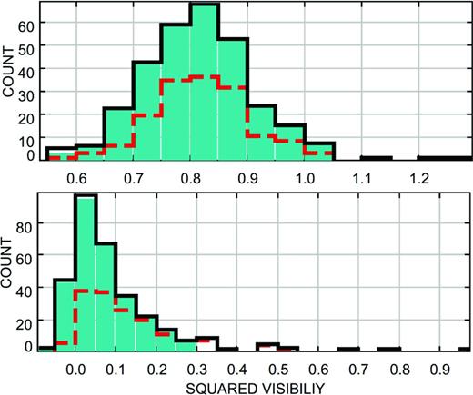
Histograms of the squared visibilities at 2.2 μm, obtained with the calibrator γ Lib (baseline A0–D0), under good (top panel) and poor (bottom panel) seeing conditions. Filled turquoise bars: final histogram after aberrant-data rejection (our method). Full black steps: initial histogram (no selection). Dashed red steps: final histogram after 50 per cent frame selection with amdlib.
Next subsection describes the weighting scheme used to average the non-aberrant data over each exposure. Note that selecting the frames with the standard amdlib procedure is equivalent to assigning unity weights to the selected frames and null weights to the others.
Computing the raw observables
To reduce the instrumental effects on the data, at the spectral channel level, we compute in each exposure (300 frames in our example) the weighted average of the squared visibility, and of the complex triple product. For the visibility, as weight associated with each frame we use the ratio of the SNR to the relative excursion of the piston, where the relative excursion of the piston itself is the ratio of the piston excursion (absolute value) for a given frame, to the average over the whole exposure. For the triple product, each individual weight is given by the geometrical mean of the three weights associated with the three baselines. The final uncertainties are derived from the variance of the distribution of the weighted means, obtained by random sampling with replacement of the original series of data (direct bootstrap method) (Efron & Tibshirani 1993). Note that our specific script computes the real and imaginary parts of the triple product, from which we extract the calibrated closure phase (see Section 4.2).
Fig. 4 shows an example of squared visibility and triple product produced by the reduction script (before calibration) from one single exposure of 300 input frames, obtained with the calibrator target γ Lib, for the three baselines A0–D0 (32 m), D0–H0 (64 m) and A0–H0 (96 m).
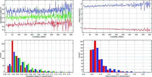
Interferometric observables given by our reduction code with the calibrator γ Lib, before calibration (good seeing). Top-left panel: squared visibilities for the baselines A0–D0 (blue), D0–H0 (green) and A0–H0 (red) w.r.t. the channel index in K. Top-right panel: real (blue) and imaginary (red) parts of the triple product for the baseline triplet A0–D0–H0. Because of their low levels, uncertainties in the bottom panels are drawn using histograms, rather than error bars (with the same colour code as the top panels).
In complement to these interferometric observables, we compute two other quantities used further in the calibration procedure (see Section 4.2.3):
the weight of each exposure defined as the product of two ratios: one is the average of the SNR to its variance; the other is the average of the inverse of the piston excursion (absolute value) to its variance and
the final number of non-aberrant data, for each spectral channel.
CALIBRATING THE DATA
The calibration process is the key point to obtain accurate estimates of the ‘true’ (intrinsic) observables of the science targets. To correct the measurements for environmental and instrumental instabilities, we observe reference stars (the calibrators), with known angular diameters and independently well-defined brightness distributions.
To calibrate the wavelength-dependent measurements obtained with VLTI/AMBER, we have developed a library of idl functions, included in the Spectrointerferometric Data Analysis Software Tool (spidast) modular software suite (Cruzalèbes, Spang & Sacuto 2008; Cruzalèbes et al. 2010), which allows one to:
link each spectral channel to a wavelength value. We use a specific method based on the correlation of calibrator measured spectra with synthetic templates given by the marcs model (Gustafsson et al. 2008) and
measure and correct for the degradation of the spatial coherence. As calibrators, we use stars with brightness distribution of limb-darkened (LD) discs, for which angular diameters are given by fits of synthetic spectra on the wide-band spectrophotometric measurements in the infrared (Cruzalèbes et al. 2010).
Computing the spectral shifts
To reach a high precision in the angular diameter estimation using model fitting, spectral calibration is a critical point (see e.g., Domiciano de Souza et al. 2008; Wittkowski et al. 2008; Stefl et al. 2011). Given the lack of any internal instrumental module for wavelength calibration in the optical setup of AMBER (Petrov et al. 2007; Robbe-Dubois et al. 2007), amdlib provides calibrated wavelength tables, computed from a theoretical polynomial dispersion law (Mérand et al. 2010), but with coefficients still badly known, leading to wavelength shifts up to ∼10 pixels in the detector plane, at medium spectral resolution (Malbet et al. 2011). To correct for this drawback, amdlib shifts the wavelength table using the correlation of the measured spectrum with a template table containing the telluric lines.
To improve the precision of the wavelength calibration, observers usually compute the coefficients of the dispersion law by identifying visually some prominent telluric lines in the measured spectrum (e.g. Kraus et al. 2009; Ohnaka et al. 2011; Weigelt et al. 2011). We propose an alternative automatic approach, based on the cross-correlation of the calibrator measured spectra with synthetic templates produced by the marcs + turbospectrum codes (Alvarez & Plez 1998; Plez 2012), including the telluric lines as well. This method was previously suggested by Plez (2003) for Gaia, and by Decin et al. (2004) or Decin & Eriksson (2007) to calibrate the Spitzer spectrograms. It is particularly suitable for stellar spectra showing easily identifiable spectral features, as it is the case with our sample of cool giant calibrators, showing strong CO bands in the 2.126–2.474 μm spectral range (Martí-Vidal et al. 2011). Fig. 5 shows the synthetic spectrum produced by the marcs + turbospectrum code, for the calibrator γ Lib. Some reference spectral lines are shown for identification of the corresponding stellar atmospheric elements.
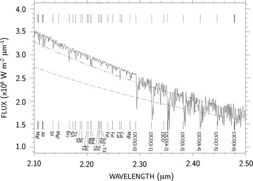
Spectral distribution of the synthetic model surface flux of γ Lib, produced by the MARCS + turbospectrum code in K. Dash–dotted line: blackbody continuous spectrum with Teff = 4660 K. Dash–triple dotted line: Engelke continuous spectrum with the same effective temperature.
For each exposure, obtained with each calibrator, and with the working instrumental setting, our automatic spectral calibration process contains the following steps:
apply the heliocentric and systemic radial velocity corrections, and multiply the synthetic spectrum by the atmospheric and instrumental transmittance profiles. Atmospheric transmission data for the southern sites (CTIO, Chile) are given by the USAF atmospheric code plexus (Cohen, Wheaton & Megeath 2003);
remove the continuum parts of the raw and synthetic spectra, and normalize the resulting spectra. As a first approximation, we estimate the continuum by decreasing the spectral resolution to |$ {\cal R}$| = 40. The main drawback of this method is to produce apparent ‘pseudo-continua’ that are lower than the real continuum levels, even in almost line-free regions (Rix et al. 2004). Since our goal is only to perform spectral calibration by correlation, this drawback has no effect on the final result;
divide the spectrum in contiguous subwindows of the same size, and compute the wavelength shift by phase correlation (Vera & Torres 2008) in each subwindow. If the spectrum is divided in n subwindows, we apply a polynomial law of degree n − 1 to correct for the wavelength shifts. Subpixel precision is obtained by embedding the cross-power spectrum in the middle of a two times larger array of zeros, before computing the phase-correlation function, by inverse Fourier transform of the final cross-power spectrum (Guizar-Sicairos, Thurman & Fienup 2008);
finds the position of the barycentre of the correlation peak for each subwindow, computes the coefficients of the interpolation law (assumed to be polynomial) and corrects the global wavelength table; and
calculates the residuals of the wavelength shifts, using once again the phase-correlation method on the wavelength-corrected spectrum.
For each observing night, the final wavelength table, associated with the working instrumental setting, is obtained by ensemble average of the corrected tables (of all exposures with all calibrators measured with the same instrumental setting), rejecting the tables showing wavelength-shift residuals higher than 8 nm (∼5 times the nominal spectral resolution). Fig. 6 shows the final continuum-corrected spectrum, given by the spectral-calibration procedure, with the calibrator γ Lib. The model spectrum drawn with the dashed line is produced by the marcs + turbospectrum code.
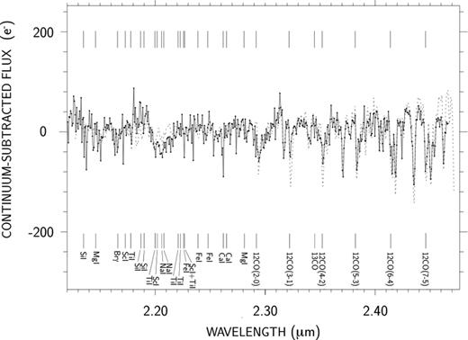
Spectral distribution of the continuum-subtracted flux of γ Lib measured with VLTI/AMBER, after spectral calibration. Dashed line: model spectrum (including tellurics).
To show the difference between the wavelength calibration provided by spidast and amdlib, we plot in Fig. 7 the corrections from the initial polynomial dispersion law of AMBER, given by the two software packages. While amdlib computes only a unique correction value applied over the whole spectrum, our method computes a polynomial correction (here parabolic from three subwindows), with subpixel deviations with respect to the polynomial law, caused by the final ensemble averaging of the corrected wavelength tables. The choice of the degree of the polynomial correction provided by spidast allows the accuracy of the wavelength correction to be adapted to the scientific programme, reaching a subpixel precision if necessary.
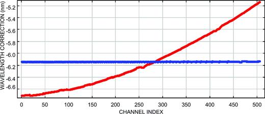
Wavelength correction from the initial polynomial dispersion law of AMBER, obtained with spidast (in red) and with amdlib (in blue), for each spectral channel of the K band (first observing night).
Calibrating spectrointerferometric data
In order to assess and correct for the measurement defects on the science targets, proper interferometric calibration (not yet fully supported with amdlib) is needed. The Instrument Response Function (IRF), also called ‘transfer function’ (Perrin 2003; van Belle & van Belle 2005; Boden 2007; Cruzalèbes et al. 2010), is derived from observations of calibrators as concomitant as possible to the ones of the science targets.
The standard calibration method is based on the assumption that a given ‘raw’ (measured) quantity q of any observable |$ {\cal Q}$|, is equal to the product of the ‘true’ (intrinsic) quantity |$\mathcal {Q}$|, multiplied by a global degradation factor |$R_ {\cal Q}$| (in other words the IRF). Such a factor cannot practically be modellized with sufficient reliability (numerous parameters and some of them remaining unknown).
Usually, calibrators are found in dedicated catalogues and the corresponding sources should meet the desired requirements. However, the number of calibrators is necessarily limited and somewhat depends on the type of science targets, so that the selected calibrators might stand out from the ideal conditions: point-like source, small angular separation and brightness matching.
In practice, the limited choice of calibrators makes it necessary to accept ‘partially’ resolved targets (van Belle & van Belle 2005), angular separations counted in degrees, and brightness mismatch amounting some units of magnitudes. For example, a bright calibrator is rarely found in a close angular vicinity of a given bright science target. Such a situation nevertheless remains convenient for the calibration procedure, since switching between science targets and calibrators is fast enough and does not affect the configuration of the interferometer, and its response as well.
This procedure starts with a first selection of calibrators via the SearchCal tool,3 created by the JMMC working group ‘Catalogue of calibration sources’, providing rough estimates for angular diameters, with comparatively large uncertainties. Following this first selection, the sources are searched in the calibrator catalogues of Bordé et al. (2002) and Mérand, Bordé & Coudé Du Foresto (2005), in order to find angular diameters of better quality. Since some calibrators do not have a diameter in the published catalogues, it is necessary to make our own determinations of those diameters (see Section 4.2.1). Moreover, in order to control these determinations and to build a homogeneous set of diameters, we apply our own method to recalculate all the diameters for the selected calibrators. The good agreement found between our determinations and the ones of the Bordé’s Catalogue of Calibrator Stars for Long-Baseline Stellar Interferometry (CCSL; as shown in Table 2 and in Fig. 8) attests to the reliability of our specific determinations of angular diameters.
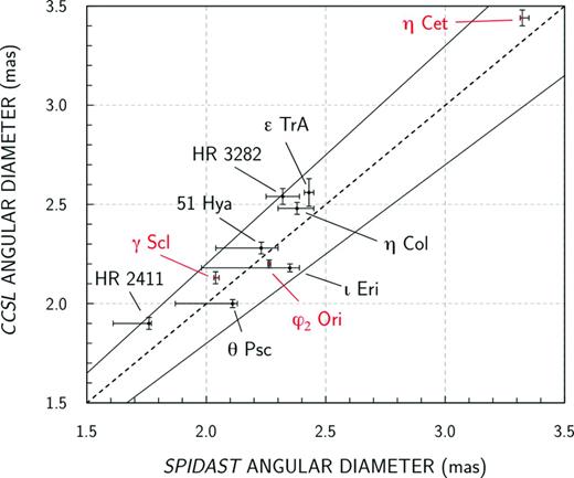
Value of the angular diameter of each calibrator of our observing sample found in the CCSL, versus the final value deduced from spidast, fitting the marcs model spectra on calibrated templates of Cohen et al. (1999) (red dots), and on IRAS-LRS measurements (black dots). Solid lines: ±10 per cent thresholds.
Science targets of our programme measured with VLTI/AMBER. Hipparcos parallaxes are in mas. The last column gives the calibrator(s) associated with each science target.
| Name | Spec. type | ϖHip | mK | Calibrator(s) |
|---|---|---|---|---|
| α Car | F0II | 10.6(6) | −1.3(3) | η Col/ι Eri/HR 3282 |
| β Cet | K0III | 33.9(2) | −0.3(4) | η Cet |
| α TrA | K2II | 8.4(2) | −1.2(1) | ε TrA/γ Lib/o Sgr |
| α Hya | K3II-III | 18.1(2) | −1.1(2) | λ Hya |
| ζ Ara | K3III | 6.7(2) | −0.6(2) | ε TrA/o Sgr |
| o1 CMa | K2.5Iab | 0.2(4) | 0.3(3) | HR 2411 |
| δ Oph | M0.5III | 19.1(2) | −1.2(2) | γ Lib/ε TrA |
| γ Hyi | M2III | 15.2(1) | −1.0(4) | α Ret |
| o1 Ori | M3III | 5.0(23) | −0.7(2) | HR 2411 |
| σ Lib | M3.5III | 11.3(3) | −1.4(2) | 51 Hya |
| γ Ret | M4III | 7.0(1) | −0.5(3) | α Ret |
| L2 Pup | M5IIIe | 15.6(10) | −1.8(1) | HR 3282/η Col |
| CE Tau | M2Iab-b | 1.8(3) | −0.9(2) | 40 Ori |
| T Cet | M5.5Ib/II | 3.7(5) | −0.8(3) | γ Scl/ι Eri |
| TX Psc | C7,2(N0)(Tc) | 3.6(4) | −0.5(3) | θ Psc |
| R Scl | C6,5ea(Np) | 2.1(15) | −0.1(1) | ι Eri |
| W Ori | C5,4(N5) | 2.6(10) | −0.5(4) | HR 2113/40 Ori |
| TW Oph | C5,5(Nb) | 3.7(12) | 0.5(4) | o Sgr/γ Lib |
Angular diameter values (in mas) of the suitable calibrators, found in the CCSL, derived from the final fit of the marcs model spectrum and found in the JSDC. The third column gives the effective temperature (in K) deduced from the spectral type, used for the model.
| Name | Spec. type | Teff | ϕCCSL | ϕfinal | ϕJSDC |
|---|---|---|---|---|---|
| α Ret | G8II-III | 4780(230) | – | 2.54|$\left(^{4}_{9}\right)$| | 2.5(2) |
| φ2 Ori | K0IIIb | 4670(230) | 2.20(2) | 2.263|$\left(^{6}_{5}\right)$| | 2.1(2) |
| η Col | K0III | 4660(230) | 2.48(3) | 2.38|$\left(^{7}_{8}\right)$| | 2.7(2) |
| λ Hya | K0III | 4660(230) | – | 2.62|$\left(^{14}_{29}\right)$| | − |
| γ Lib | K0III | 4660(230) | – | 2.31|$\left(^{7}_{15}\right)$| | − |
| o Sgr | K0III | 4660(230) | – | 2.50|$\left(^{12}_{27}\right)$| | 2.4(2) |
| ι Eri | K0.5IIIb | 4600(220) | 2.18(2) | 2.35|$\left(^{4}_{37}\right)$| | 2.5(2) |
| θ Psc | K0.5III | 4580(220) | 2.00(2) | 2.11|$\left(^{2}_{24}\right)$| | 2.1(2) |
| γ Scl | K1III | 4510(220) | 2.13(3) | 2.039|$\left(^{14}_{7}\right)$| | 2.2(2) |
| HR 2113 | K1.5III | 4440(220) | – | 2.48(2) | 2.4(2) |
| ε TrA | K1.5III | 4440(220) | 2.56(7) | 2.43(2) | − |
| η Cet | K1.5III | 4440(220) | 3.44(4) | 3.323|$\left(^{28}_{9}\right)$| | 3.3(2) |
| HR 3282 | K2.5II-III | 4330(210) | 2.54(4) | 2.32(7) | − |
| HR 2411 | K3III | 4260(210) | 1.90(3) | 1.76|$\left(^{1}_{15}\right)$| | − |
| 51 Hya | K3III | 4260(210) | 2.28(3) | 2.23|$\left(^{7}_{19}\right)$| | 2.4(2) |
Determining calibrator angular diameters
To derive the IRF for each spectrointerferometric (SPI) observable, we first need to get a reliable estimate of the angular diameter of each calibrator, and its associated error. Fitting the stellar models of Kurucz (1979) on the absolutely calibrated spectrophotometric templates of Cohen et al. (1999), the CCSL contains 374 calibrators, with LD angular diameters ranging from 1 to 3 mas. Since our selected calibrators might have no angular diameter estimate (one-third of the calibrators of our data set have no value found in the catalogues), or poorly estimated, we have added to spidast various routines for determination of the angular diameter from indirect methods, presented in detail in Cruzalèbes et al. (2010). These routines compute the angular diameter:
by combining the linear diameter, deduced from absolute luminosity and effective temperature from the Morgan Keenan (MK) spectral type, with the parallax;
by using experimental laws based on the interstellar-corrected colour index (surface brightness method);
by scaling synthetic spectra on broad-band photometric measurements (infrared flux method); and
by fitting synthetic spectra on infrared spectrophotometric measurements (see Section 6).
Table 2 gives the angular diameter values of our calibrators found in the CCSL, as well as our final estimates, derived from the fit of marcs + turbospectrum synthetic spectra on photometric or spectrophotometric measurements. In the last column, we also give the estimates found in the JMMC Stellar Diameter Catalogue (JSDC) of Lafrasse et al. (2010), with accuracies between 7 and 10 per cent (Delfosse 2004; Bonneau et al. 2006).
Fig. 8 shows the comparison of our estimates with the CCSL values. The mean difference between our estimates and the CCSL is 5 per cent. The mean difference for the three targets with the available calibrated templates of Cohen (i.e. ϕ2 Ori, γ Scl and η Cet) is lower: 3.5 per cent. This shows the satisfactory agreement between our results and the CCSL, which confirms the reliability of our approach for determination of the calibrator angular diameters, implemented in spidast.
Modelling the calibrator visibility and triple product
Once we determined the angular diameter of each calibrator, and its associated uncertainty, we derive the IRF for each SPI observable, computing the ratio of the observable measured on the calibrator, to the synthetic observable, assumed to represent the ‘true’ calibrator observable. Each synthetic SPI observable is derived from the synthetic coherent flux |$C_{\lambda }^\mathrm{model}$|:
the synthetic flux (equation 1) is given by the synthetic coherent flux computed for the null baseline (visibility unity);
the squared synthetic visibility (equation 2) by the ratio of the squared synthetic coherent flux to the synthetic squared flux;
the synthetic bispectrum (equation 3) by the product of the synthetic coherent flux for the three baselines composing each triplet; and
and the synthetic triple product (equation 4) by the ratio of the synthetic bispectrum to the cubed synthetic flux.
Since compact photospheres are known to deviate from simple uniform discs (see Hajian et al. 1998, and references therein), radially decreasing from their photometric centre, we use the marcs + turbospectrum codes to produce models of Centre-to-Limb Variation (CLV) profiles, with input parameters derived from the MK spectral type. Fig. 9 shows the λ-μ map of typical CLV profiles given by the model, where the reduced radial coordinate μ is given by |$\mu = \sqrt{1-r^2}$| (Young 2003).
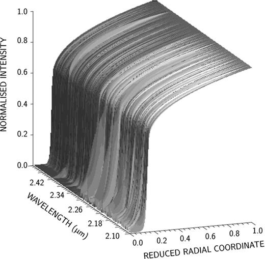
λ–μ map of CLV profiles produced by the marcs + turbospectrum code, in the K band, for a K0III-type star.
With ‘partially’ resolved calibrators, the deviation from the uniform-disc (UD) model increases with the baseline length. Fig. 10 shows the squared visibility and the real part of the triple product produced by the marcs and the UD models, for the calibrator η Ceti (ϕfinal = 3.32 ± 0.02 mas), deduced from measurements obtained with the D0–I1–G1 baseline triplet (G1–I1 = 46 m, D0–G1 = 69 m and D0–I1 = 79 m). In this example, the differences in visibility and triple product between the UD model and the LD-marcs model are larger than the uncertainty of the synthetic observables (derived by propagating the uncertainty on the angular diameter), hence, it is justified to use the LD model instead of the UD model.
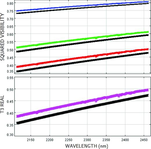
Theoretical interferometric observables of the calibrator η Ceti, produced by the LD-marcs model (in colour), and by the UD model with the same value of the angular diameter (in black). Top panel: squared visibilities for the baselines G1–I1 (blue), D0–G1 (green) and D0–I1 (red). Bottom panel: real part of the triple product produced by the models, for the baseline triplet D0–G1–I1. For each curve, the thickness gives the uncertainty.
Correcting for the degradations of the IRF
The main source of non-stationary instabilities which affects the fringe formation is the atmospheric-phase turbulence (Roddier 1981). This issue is partially solved thanks to the use of fringe-tracking servo-loops scanning the fringes with cycle periods smaller than the seeing coherence time, defined as the time over which the phase fluctuations remain coherent (Davis & Tango 1996; Kellerer & Tokovinin 2007). Thus, the residual instabilities are expected to cause only slow drifts of the IRF between observations of the science targets and their associated calibrators. In order to estimate the response at the time when each science target is measured, linear interpolation between the successive measurements on its calibrator(s) is legitimate (Perrin 2003), provided that the ‘calibrator-science-calibrator’ observation sequence repeated several times and rapidly samples the evaluation of the IRF (Berger, Dumas & Kaüfer 2011).
To perform the calibration of the squared visibility and triple product data, spidast applies the following procedure, working at spectral channel level.
Compute the measured IRF for each exposure, given by the ratio of the calibrator measured observable to the calibrator synthetic observable (at the same spectral resolution, for the same baseline or baseline triplet). Values and uncertainties are derived from the fourth-order approximation formulae of Winzer (2000). For triple product data, the approximation formulae apply separately to the real and imaginary parts of the complex ratio. Since the calibrator angular diameter uncertainties are smaller than 10 per cent (see Table 2), the uncertainty of a model observable is simply obtained from its first partial derivative w.r.t. the angular diameter, multiplied by the angular diameter uncertainty.
Average the IRF measurements over each OB. As weight is associated with each exposure, we use the ratio of the associated weight (defined in Section 3.2) to the variance of the calibrator ‘raw’ observable.
Determine the IRF at the mean time of each exposure obtained with the science target from linear interpolation, or polynomial fit, on the averaged IRF measurements. Fig. 11 shows the temporal variation of the measured and interpolated response in squared visibility and triple product, obtained during one observing night, with three successive calibrators.
Divide the observable measured on the science target for each exposure of a given OB, by each interpolated value of the IRF obtained for the same OB (using Winzer’s formulae). Applying a method similar to that used with the getCal tool of the Cal. Inst. Tech. (2008), a weight is associated with each calibrated ratio, which combines information on the observations of the calibrator and of the science target (science–calibrator angular separation and observation-time delay, coherence time and number of non-aberrant data).
Compute the weighted average over each OB of the ratios used in the calibration, which gives the final calibrated SPI observable (see Section 4.2.4). The argument of the final calibrated triple product gives the final calibrated closure phase.
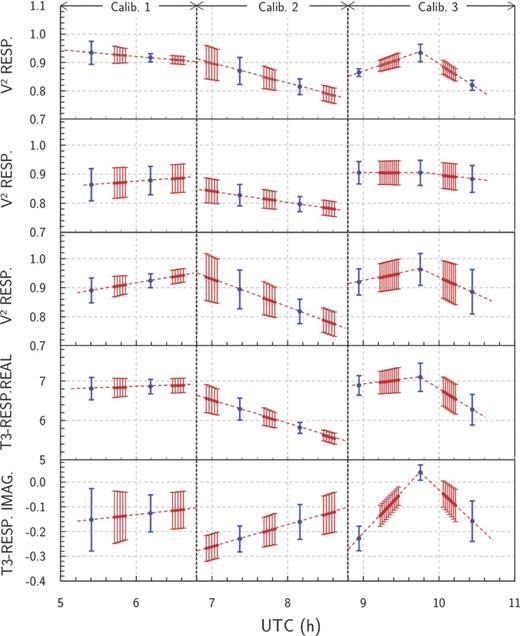
Temporal variation of the IRF (λ = 2.2 μm) during one observing night. Blue dots: response values averaged over each OB, successively obtained with the calibrators γ Lib, ε TrA and o Sgr. Red dots: response values interpolated at the time of observation of the science targets (red dashed lines: interpolated response). From top to bottom: response in squared visibility for the baselines A0–D0, D0–H0, A0–H0, real and imaginary parts of the response in triple product for the triplet A0–D0–H0.
Although the calibration procedure used by spidast is based on the standard calibration method, great care has been taken to provide reliable uncertainty estimates, thanks to the use of weights tracing the data quality at different levels of the processing. Thus, spidast produces large uncertainties on final calibrated observables obtained with input data of poor quality. Estimating reliable error bars is of crucial importance to get calibrated data, usable for the fitting process of parametric models, even on data of uneven quality (see Section 6).
Comparing the final calibrated observables with amdlib
Although the calibration routine provided with the amdlib package is not yet officially validated (Malbet et al. 2011), we compute the differences in squared visibility and closure phase between spidast and amdlib, and compare them with the associated uncertainties.
Fig. 12 shows the results obtained on the science target δ Oph, with the baseline triplet A0–D0–H0, under good and poor seeing conditions. The histograms of the uncertainties show that the uncertainties in squared visibility estimated with amdlib are smaller than with spidast (whatever the seeing), while it is the contrary for the uncertainties in closure phase.
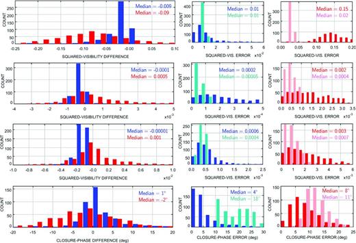
Histograms of calibrated quantities pertaining to the science target δ Oph, obtained in good (blue) and poor (red) seeing conditions. From top to bottom: squared visibilities with the baselines A0–D0, D0–H0, A0–H0 and closure phase with the triplet A0–D0–H0. Long panels of the first column: difference between spidast and amdlib. Small panels of the other columns: associated uncertainties with good (blue: spidast, turquoise: amdlib) and poor seeing (red: spidast, pink: amdlib).
To explain the disagreement between the uncertainties in squared visibility, we remind that spidast takes into account instrumental and environmental conditions in the calculation of the uncertainties, while amdlib uses only unweighted variance. Thus, we consider as underestimated the uncertainties in squared visibility produced by amdlib.
Regarding the closure phase, it is more difficult to explain why the uncertainties from amdlib are larger than the ones from spidast. Indeed, no details are found in Malbet et al. (2011), expected to describe the amdlib calculation. spidast computes the uncertainties on the real and imaginary parts of the calibrated triple product, and derives the uncertainties on the final closure phase from them. A deep analysis based on the source code of the calibration routine provided by amdlib reveals that amdlib computes the uncertainties in the final closure phase, adding the uncertainties in closure phase of the science target and of the estimated transfer function. Since the closure phase is less stable than the triple product, the final uncertainties in closure phase handled with amdlib are larger than with spidast.
To evaluate the agreement between the two procedures, we compare the differences between the final calibrated SPI observables they produce to the associated uncertainties. Since the median differences are smaller than the median uncertainties (Fig. 12), we conclude that the agreement between the two software packages is satisfactory, spidast giving more reliable uncertainties than amdlib.
MEASURING THE DEVIATION FROM CIRCULAR SYMMETRY
The closure phase ψ123 couples the phases φ of the Fourier transform of the source brightness distribution at the three spatial frequencies f1, f2 and f3 = f1 + f2, probed by the three baselines in the following way: ψ123 = φ(f1) + φ(f2) − φ(f3). In the case of a centrosymmetrical brightness distribution on-axis, the phase of the Fourier transform is uniformly zero and ψ123 is naturally equal to zero. If this source is off-axis, the phase is linear w.r.t. the spatial frequency, so that φ(f3) = φ(f1) + φ(f2), and, subsequently, also here ψ123 is equal to zero. Thus, a non-zero phase closure is a clear indication, at least qualitatively, for a deviation from circular symmetry.
In Section 5.2, we introduce a new parameter (called the centrosymmetry parameter, CSP), based on the triple product, more sensitive to deviation from centrosymmetry than the closure phase.
Global closure phase
CSP values and global closure phases for the science targets. The last column gives the ratio of the associated SNRs.
| Name | CSP (°) | ψband (°) | SNRCSP/SNRψ |
|---|---|---|---|
| δ Oph | 0.76(3) | 0.16(4) | 7.0 |
| α Car | 0.84(3) | −0.22(5) | 5.7 |
| L2 Pup | 0.90(4) | 0.39(5) | 3.2 |
| β Cet | 0.98(4) | 0.32(6) | 4.6 |
| ζ Ara | 1.12(4) | −0.22(6) | 8.1 |
| α TrA | 1.21(5) | 0.20(7) | 8.3 |
| α Hya | 1.21(9) | −0.16(11) | 9.4 |
| TW Oph | 2.94(5) | −2.91(5) | 1.1 |
| CE Tau | 3.01(11) | −0.85(17) | 5.5 |
| γ Hyi | 3.25(11) | 2.83(13) | 1.4 |
| o1 CMa | 4.41(197) | 2.88(155) | 1.2 |
| σ Lib | 5.12(20) | −1.90(33) | 4.4 |
| γ Ret | 5.16(37) | −4.44(115) | 3.6 |
| TX Psc | 5.34(25) | −2.17(32) | 3.4 |
| o1 Ori | 8.10(82) | 7.48(84) | 1.1 |
| W Ori | 10.58(46) | 1.35(79) | 13.3 |
| R Scl | 11.63(59) | −10.63(67) | 1.2 |
| T Cet | 27.88(51) | −28.79(41) | 0.8 |
Centrosymmetry parameter
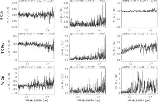
Left-hand panels: spectral variation of the imaginary part of the triple product, divided by the spectral average of the real part, for three science targets (the ‘spectral mean’ quoted above each panel corresponds to the spectral average of the displayed quantity; for the left-hand panels, it thus equals the tangent of the global closure phase). Central panels: absolute value of the imaginary part of the triple product, divided by the spectral average of the modulus (for the central panel, the ‘spectral mean’ equals the sinus of the CSP). Right-hand panels: absolute value of the real part of the triple product, divided by the spectral average of the modulus.
To illustrate the difference between the global closure phase and the CSP, we plot in Fig. 13 three quantities, for three scientific targets showing a global closure phase close to zero,
in the panels on the left is shown the imaginary part of the triple product |$\Im {\cal T}_\mathrm{true}$|, divided by the spectral mean4 of the real part |$\left\langle \Re {\cal T}_\mathrm{true}\right\rangle$|. Note that the spectral mean of this ratio is equal to the tangent of the global closure phase, as defined in equation (8);
in the panels forming the central column is shown the absolute value of the imaginary part of the triple product |$\left|\Im {\cal T}_\mathrm{true}\right|$|, divided by the spectral mean of the modulus |$\left\langle \left| {\cal T}_\mathrm{true}\right|\right\rangle$|. Note that the spectral mean of this ratio is equal to the sine of the global CSP, as defined in equation (9); and
in the panels on the right is shown the absolute value of the real part of the triple product |$\left|\Re {\cal T}_\mathrm{true}\right|$|, divided by the spectral mean of the modulus |$\left\langle \left| {\cal T}_\mathrm{true}\right|\right\rangle$|.
The three panels on the left show three typical behaviours for |$\Im {\cal T}_\mathrm{true}$| :
uniformly close to zero (δ Oph);
decreasing symmetrically around zero (TX Psc); and
increasing symmetrically around zero (W Ori).
For each of these situations, the integration over the spectrum produces a nearly null result (hint for centrosymmetry). However, the CSP allows to detect deviations from centrosymmetry (see Fig. 14).
If the real and imaginary parts of the triple product are wavelength independent, for the observation spectral range, one can show that sin CSP = |ψband|. If not, no analytical relation linking the two quantities can be derived from equations (8) and (9), because of the integrals in the numerators and the denominators. Fig. 14 shows the CSP in K displayed versus the global closure phase in the same spectral band, for each science target, choosing the OB which gives the smallest uncertainty on the CSP. Almost all the stars fall along the diagonals of the (ψband, CSP) diagram, which trace the relation CSP = |ψband|. One (W Ori), however, is flagged as asymmetrical with the CSP indicator, but not with ψband. This is precisely why we favour the CSP over ψband, as discussed above. T Cet has the largest values for CSP and ψband as well, indicating large deviation from centrosymmetry (may be due to strong asymmetries at the wavelengths of the CO bands or even suggestive of the presence of a binary companion). The second largest CSP value pertains to R Scl, recently revealed as a wide binary by Maercker et al. (2012), using the ALMA array at millimetric wavelengths. In addition, the last column of Table 3 shows that, except for T Cet, the SNR for the CSP is comparable to or larger than the SNR for the global closure phase.
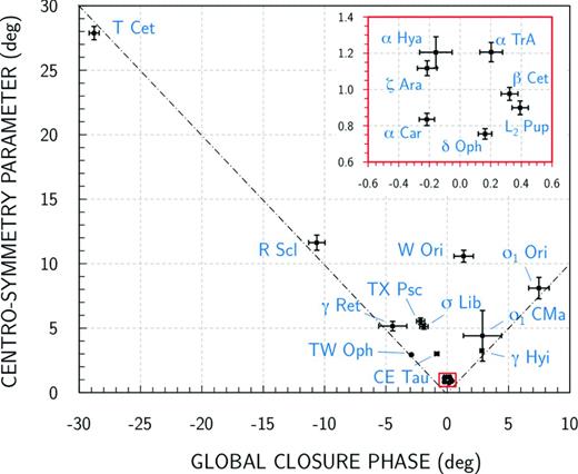
The CSP versus ψK, the global closure phase in K, for the science targets. The red inset in the upper-right corner enlarges the group of points located at the bottom, around the null value of the global closure phase, pertaining to the targets δ Oph, α Car, L2 Pup, β Cet, ζ Ara, α TrA and α Hya. The dash–dotted diagonals trace the relation CSP = |ψK|.
FITTING PARAMETRIC CHROMATIC MODELS
In order to interpret the final calibrated SPI observables, spidast provides a fitting routine, based on the modified gradient-expansion algorithm, very similar to the algorithm invented by Levenberg (1944), and improved by Marquardt (1963). The fit applies on any calibrated SPI measurements (to be chosen between visibility, flux, coherent flux, bispectrum, triple product and closure phase), using a library of single-component or composite parametric chromatic models, characterized by the Fourier spectrum of their intensity distribution, and the associated first-order partial derivatives w.r.t. the model parameters. Fig. 15 shows examples of visibility-fitting results obtained with spidast, using two models (UD and LD-marcs). This fitting routine, applied on spectrophotometric data, is used to determine the calibrator angular diameters from the marcs + turbospectrum synthetic spectra (see Section 4.2.1).
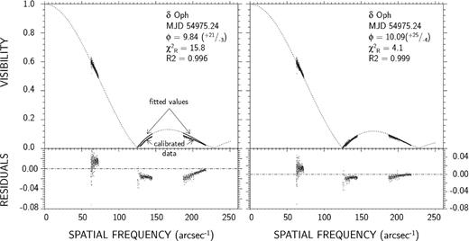
Fits on the visibility data of δ Oph obtained with the baselines A0–D0, D0–H0 and A0–H0, for one single OB. Left-hand panel: fit of the UD model; right-hand panel: fit of the LD-marcs model (models in dashed lines). Calibrated data are shown without error bars, for clarity purpose. ϕ is the best-fitting angular outer diameter (in mas), |$\chi ^{2}_\mathrm{R}$| the reduced χ2 and R2 the adjusted coefficient of determination. Bottom panels: residuals (calibrated data-fitted values).
Note that the litpro software,5 developed by the JMMC working group ‘Model fitting’, uses a set of elementary geometrical and centre-to-limb darkening functions as well (Tallon-Bosc et al. 2008). However, it does not offer, contrary to spidast, the possibility to fit stellar-disc models with synthetic tabulated radiance data (or exitance, for fits on spectrophotometric measurements), such as those produced by the marcs + turbospectrum code.
Since the uncertainties of the final calibrated data are not normally distributed, the covariance matrix, that comes out of the χ2 fit, cannot be used to infer the parameter uncertainties (Press et al. 2007). To compute the uncertainties, spidast uses the residual-bootstrap method, described in detail in Cruzalèbes et al. (2010):
‘synthetic’ data sets are produced from random sampling with replacement of the Pearson residuals (difference between calibrated and fitted values divided by the uncertainty of the observed value), added to the initial fitted values;
fitting the model on these new data sets produces a set of χ2 minima, following a probability distribution, from which we extract the boundaries of the confidence interval, with a given confidence level; and
the parameter values associated with these χ2 boundaries give the upper and lower limits of the parameter estimates, leading to asymmetric uncertainties.
The whole procedure allows the computing of reliable estimates of the parameter uncertainties.
CONCLUSION
In this paper, we introduce the new spidast software, developed since 2006 with the aim to reduce, calibrate and interpret the visibility and triple product measurements obtained with the VLTI/AMBER facility. spidast contains a whole set of modules, which can be launched separately or in an automatic batch file, and summarized hereafter.
The raw data reduction used by spidast computes the weighted average of non-aberrant data, at spectral-channel level, providing estimates of the SPI observables using an automated procedure, while the method presently used with amdlib selects the ‘best’ frames according to a quality threshold determined a posteriori, after several trials.
The wavelength calibration procedure performed by spidast provides spectral shifts following a polynomial law, tracing them at the channel level. This is done by computing the cross-correlation of the measured spectra of the calibrators with their synthetic spectra produced by the marcs model, while amdlib only provides a constant spectral shift over the spectrum, from the correlation with the telluric lines.
For selected calibrators not included in the calibrator catalogues, spidast provides several routines for estimation of the angular diameter with indirect methods, the most accurate being the fit of stellar-atmosphere model spectra given by marcs on spectrophotometric data. The calibrator synthetic observables are derived using CLV functions produced by marcs.
To obtain an accurate interferometric calibration (via an automated procedure), spidast: (1) divides the calibrator raw data with the associated synthetic observables in each spectral channel, which gives the instrumental response function in squared visibility and triple product; (2) interpolates or fits the response at the time of each exposure on the science target; (3) divides the science raw data with the interpolated/fitted response, which gives the science calibrated observables for each exposure; and (4) computes their weighted average over each OB. At each processing step, the uncertainties are computed, thanks to the bootstrap method applied on the weighted means.
Using the real and imaginary parts of the calibrated triple product, spidast measures the deviation from centrosymmetry of the brightness distribution of each science target in the observation spectral band, thanks to a new parameter, more sensitive to asymmetries than the global closure phase.
Finally, spidast proposes a complete fitting tool, using a set of parametric and chromatic models, and accepting input tables of flux/intensity synthetic data.
Such a careful calibration process of SPI data is a crucial step for their trustworthy astrophysical exploitation, which is the topic of two associated papers (Cruzalèbes et al., in preparation). Parameter extraction using non-linear fits of source model, as well as aperture-synthesis image reconstruction, need reliable estimates of the calibrated observables, with robust uncertainties. Our reduction, calibration and fitting routines also apply to any other spectral data sets, including spectroscopic data. We made the spidast software public:6 the source code of any program of our software suite can be obtained by sending an e-mail to the first author of this paper.
The authors thank the ESO-Paranal VLTI team for supporting their AMBER observations, especially the night astronomers A. Mérand, G. Montagnier, F. Patru, J.-B. Le Bouquin, S. Rengaswamy, and W. J. de Wit, the VLTI group coordinator S. Brillant, and the telescope and instrument operators A. and J. Cortes, A. Pino, C. Herrera, D. Castex, S. Cerda, and C. Cid. They also thank the Programme National de Physique Stellaire (PNPS) for supporting part of this collaborative research. AJ is grateful to B. Plez, K. Eriksson and T. Masseron for their ongoing support on the use of the marcs code. SS was (partly) supported by the Austrian Science Fund through FWF project P19503-N16; AC is post-doctoral fellow from F.R.S.-FNRS (Belgium; grant 2.4513.11); and EP is supported by PRODEX. The data were partially reduced using the publicly available data reduction software package amdlib, kindly provided by the Jean-Marie Mariotti Center. This study used the SIMBAD and VIZIER data bases at the CDS, Strasbourg (France), and NASAs ADS bibliographic services.
Applied on observations made with ESO telescopes at the Paranal Observatory under Belgian VISA Guaranteed Time programme ID 083.D-029(A/B), 084.D-0131(A/B) and 086.D-0067(A/B/C).
Defined as the integral w.r.t. the wavelength, divided by the spectral bandwidth Δλ = λmax − λmin.
