


Abstract
We present the results of a comparative period search on different time-scales and modelling of the ZZ Ceti (DAV) star GD 154. We determined six frequencies as normal modes and four rotational doublets around the ones having the largest amplitude. Two normal modes at 807.62 and 861.56 μHz have never been reported before. A rigorous test revealed remarkable intrinsic amplitude variability of frequencies at 839.14 and 861.56 μHz over a 50 d time-scale. In addition, the multimode pulsation changed to monoperiodic pulsation with an 843.15 μHz dominant frequency at the end of the observing run. The 2.76 μHz average rotational split detected led to a determination of a 2.1 d rotational period for GD 154. We searched for model solutions with effective temperatures and log g close to the spectroscopically determined ones. The best-fitting models resulting from the grid search have MH between 6.3 × 10⁻⁵ and 6.3 × 10⁻⁷M*, which means thicker hydrogen layer than the previous studies suggested. Our investigations show that mode trapping does not necessarily operate in all of the observed modes and the best candidate for a trapped mode is at 2484 μHz.
1 INTRODUCTION
It has been well established that g-mode white dwarf pulsators show diversity in light variation from the simple sinusoidal to the mightily complicated ones. The latter variation is accompanied by non-linear features due to harmonics and combination frequencies (see e.g. the review of Fontaine & Brassard 2008).
It has also been pointed out that pulsational amplitudes and/or the frequency content of light curves might vary on short time-scales. These phenomena are quite common amongst the cooler DAVs and DBVs, and also the planetary nebula nucleus variable stars (Handler 2003). The amplitude variability can be helpful to asteroseismology as different normal modes become detectable over time, and therefore the number of known modes increases (see e.g. the case of G29-38; Kleinman et al. 1998). However, amplitude variations on time-scales of weeks and months can make the accurate determination of individual modes difficult or even impossible using the standard Fourier deconvolution technique. These variations occur sometimes as sudden effects as in the case of the ‘ever-changing’ GD 358, the most spectacular representative of the phenomenon (Kepler et al. 2003; Provencal et al. 2009). In spite of intense observational efforts, the origin of these phenomena still remains unknown. A possible explanation, which can be tested relatively easily, is mode beating due to different unresolved pulsational modes (such as rotational splitting).
The DAVs lying near the red edge of the ZZ Ceti instability strip (GD 154 is an example) are characterized by long periods and complex pulsational behaviour. Changes in pulsation from a single-mode status (connected by harmonics and not trivially by subharmonics) to a multimode status have been seen for GD 154 during the previous observations. Since the seemingly new appearance of a different normal mode can be caused only by the amplitude variation of the ever excited normal modes, we decided to follow the pulsational behaviour for an observational season. We present our comparative analyses on different time-scales. It was the increased number of pulsational periods determined by our data set that allowed us to investigate the star from an asteroseismological point of view. We also discuss the related results in the paper.
2 OBSERVATIONS AND DATA REDUCTION
We used the 1 m Ritchey–Chrétien Coudé telescope at Piszkéstető mountain station of Konkoly Observatory for data collection on GD 154. The observations were made with a Princeton Instrument VersArray:1300B back-illuminated CCD camera without any filter. Our observing season spanned six months in 2006. Altogether, 90 h of photometric data were collected on 19 nights. 30 s integration times were used. The longest continuous single-night light curve was more than 9 h long. The shortest one that we found useful to determine the frequency content covers two full cycles. Details of the observations are provided in Table 1.
Log of observations of GD 154. Five subsets were created based on the closely spaced nights.
| Run | Subset | ut date | Start time | Points | Length |
|---|---|---|---|---|---|
| no. | no. | (2006) | (BJD-245 0000) | (h) | |
| 01 | 1 | Feb 03 | 3769.520 | 372 | 4.04 |
| 02 | 1 | Feb 05 | 3771.575 | 335 | 3.28 |
| 03 | 1 | Feb 07 | 3773.519 | 340 | 4.06 |
| 04 | 2 | Mar 02 | 3797.430 | 585 | 5.66 |
| 05 | 2 | Mar 06 | 3801.481 | 484 | 4.72 |
| 06 | 2 | Mar 07 | 3802.285 | 787 | 9.11 |
| 07 | 2 | Mar 08 | 3803.305 | 684 | 6.60 |
| 08 | 3 | Mar 31 | 3826.364 | 659 | 6.60 |
| 09 | 3 | Apr 02 | 3828.288 | 291 | 5.03 |
| 10 | 3 | Apr 04 | 3830.357 | 451 | 4.42 |
| 11 | 4 | Apr 21 | 3847.385 | 493 | 5.45 |
| 12 | 4 | Apr 22 | 3848.321 | 709 | 6.88 |
| 13 | 4 | Apr 23 | 3849.316 | 549 | 6.85 |
| 14 | 4 | Apr 24 | 3850.380 | 468 | 5.20 |
| 15 | 4 | Apr 25 | 3851.332 | 541 | 6.44 |
| 16 | 5 | Jul 13 | 3930.340 | 65 | 0.71 |
| 17 | 5 | Jul 17 | 3934.335 | 92 | 1.06 |
| 18 | 5 | Jul 18 | 3935.336 | 161 | 1.83 |
| 19 | 5 | Jul 19 | 3936.342 | 150 | 1.65 |
| Total: | 8216 | 90.19 |
The original images were reduced using standard iraf1 routines. Bias, dark and flat corrections were applied on the frames. We performed aperture photometry using the iraf daophot package, setting the aperture size to two times the average full width at half-maximum on the given night, and applied differential photometry on the stars. All the time data were calculated to Baricentric Julian Date (BJD).
We obtained BVRI photometry and checked the B − V indices of the potential comparison stars on the frames, but we found that they were rather different from the value of GD 154 (B − V = 0.18). As there was no candidate for a comparison star with similar colour to our target, we tested all the stars on our CCD field by computing the average magnitudes to construct a reference light curve. We found that the most constant signal with the lowest standard deviation value could be constructed by averaging the data of the three brightest stars around the variable (see Fig. 1). A part of a differential light curve of the reference system and a check star's (C1) averaged data is presented in Fig. 2. We applied the widely used polynomial fitting method to remove the effect of the atmospheric extinction. The low-frequency part of the Fourier transform is biased by this filtering (up to 20–30 d−1), for which reason we did not focus on low frequencies in our Fourier analysis.
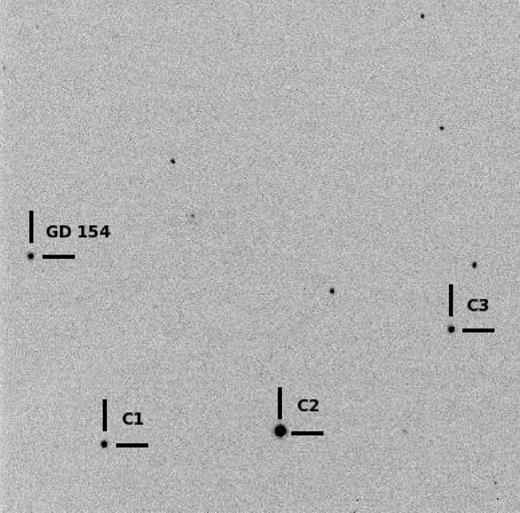
The CCD field with the variable and the comparison stars. The marked stars C1, C2, C3 were used to construct a reference light curve.
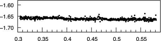
Differential light curve of C1 to the average of the three reference stars is shown (C1, C2, C3), obtained on JD 245 3803. The standard deviation is 0.003 mag.
3 FREQUENCIES IN GD 154
The light curves of GD 154 during 2006 can be seen in Fig. 3. The different minimum to maximum amplitude of the cycles suggests an overall multimode behaviour, except for the regular cycles of the last nights. To get an overall view of the pulsation modes of GD 154, we present here the modes determined in different epochs.
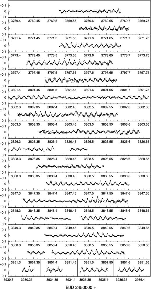
Normalized differential light curves of the 19-night run on GD 154.
3.1 Frequencies in the previous data
The light variation of GD 154 was discovered in 1977 by Robinson et al. (1978). The star showed non-linear monoperiodic pulsation with F = 843 μHz main frequency, harmonics (2F, 3F, 4F, 5F) and ‘intermediate frequencies’ (1.52F, 2.53F, 3.53F). The pulsation was regular except on the last night of the observations, when the light curve changed dramatically as the 1.52F mode became dominant. The authors suggested that the energy exchanged between the two modes due to weak non-linearity.
The existence of the near half-integer frequencies in the power spectra is not unique. Similar pulsational behaviour was observed in PG 1351+489 (DBV; Goupil, Auvergne & Baglin 1988) and in G191−16 (DAV; Vauclair et al. 1989). According to a possible explanation, an independent g-mode can be excited near 1.5F, as we see in the interpretation of the data obtained on BPM 31594 (O’Donoghue, Warner & Cropper 1992).
The Fourier spectral features and the sudden change in the dominant period made GD 154 interesting enough to be the target of the Whole Earth Telescope (WET; Nather et al. 1990) campaign in 1991. The 12 d quasi-continuous observations and the follow-up campaign organized a month later resulted in another interpretation of the pulsation. Three independent modes (f1 = 842.8 f2 = 918.6, f3 = 2484.1 μHz) and their triplet components were found in the data set. All the other peaks in the power spectra were explained as linear combinations and harmonics. Non-linear behaviour was clearly confirmed but no drastic period change was observed. Surprisingly, they did not find peaks around half-integer frequencies (Pfeiffer et al. 1996).
In 2004, an analysis of a two-site observational campaign (Hürkal et al. 2005) reported changes in the frequency and amplitude content. Some additional frequencies appeared; however, none was near the subharmonic. They were interpreted as new excited modes at 786.5, 885.4 and 1677.7 μHz. However, the authors did not find the frequencies at 842.8 and 918.6 μHz that were observed before.
We can summarize that although four modes (786.5, 842.8, 885.4 and 918.6 μHz) were reported in a 132 μHz range, not more than two were present during a given observing run. None of them was present in every data set, although one of them (≈843 μHz) was present in 1977 (Robinson et al. 1978) and in 1991 (WET campaign; Pfeiffer et al. 1996) with nearly the same value. The different solutions raise the possibility that (1) different modes are excited from time to time or (2) their amplitude is changing to below or above the detection limit, or (3) the actual frequency content interfering with the alias patterns of a given data distribution results in a seemingly changeable frequency content.
3.2 Analyses of the new data
A standard frequency analysis was performed with the Multi-Frequency Analyzer (MUFRAN) time-string tool (Kolláth 1990; Csubry & Kolláth 2004). The software package is a collection of methods for period determination, sine-wave fitting for observational data and graphic routines for visualization of the results. In each step, a fine tuning of the actual multifrequency solution was carried out to avoid the disadvantage of pre-whitening. At the same time, both the amplitudes and the fit were checked to avoid any misidentification of a peak as a real frequency. Investigations for significance and errors were obtained with the period04 package (Lenz & Breger 2005).
The Fourier spectrum of our whole data set (over 167 d) revealed the complexity of the resolution based on a set of single-site observations (Fig. 4).
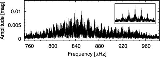
Fourier spectrum of the whole data set. The window function is given in the inset.
The overall appearance, a pyramid-like feature, suggests that more frequencies are present in the 760–960 μHz frequency range. The fine structure is more complicated than the spectral window (inset in Fig. 4) and suggests that the amplitude of the modes may have changed during the whole timebase.
We carried out comparative analyses on different time-scales (weeks and a whole observational season) that resulted in different spectral window patterns. On a medium-size time-scale (regularity of telescope allocation), the frequency resolution is acceptable, and the amplitude variation is still not masked. The baseline of the whole data set gives a better resolution, but the amplitudes are not correct when amplitude variation is going on in a shorter time-scale.
Concerning the 760–960 μHz frequency region, 12 frequencies were identified in the whole data set, and are given in Table 2 (columns 2 and 3). The 0.035 μHz Rayleigh frequency of the whole data set guaranteed that the frequencies are properly resolved. According to the frequency differences, three triplets, a doublet and a single frequency were found. We confirmed the frequencies found previously, except the one at 786.45 μHz given by Hürkal et al. (2005). Our new discoveries are two modes at 807.62 and 861.56 μHz values. The increased number of normal modes puts more constraints for modelling.
The frequency content of the whole data and two subsets.
| Mode | Whole data | Second subset | Fourth subset | |||
|---|---|---|---|---|---|---|
| Freq. | Ampl. | Freq. | Ampl. | Freq. | Ampl. | |
| No. | (μHz) | (mmag) | (μHz) | (mmag) | (μHz) | (mmag) |
| 1 | 839.14 | 9.16 | 838.92 | 16.19 | 838.53 | 6.00 |
| 2 | 843.15 | 9.46 | – | – | 843.50 | 4.07 |
| 3 | 844.65 | 7.22 | 845.17 | 3.82 | – | – |
| 4 | 861.56 | 7.31 | – | – | 861.52 | 13.04 |
| 5 | 864.27 | 4.23 | – | – | 863.98 | 4.39 |
| 6 | 857.84 | 4.37 | – | – | – | – |
| 7 | 807.62 | 3.99 | – | – | – | – |
| 8 | 802.94 | 3.97 | – | – | 802.93 | 5.81 |
| 9 | 809.20 | 3.76 | 809.77 | 8.33 | 810.17 | 3.18 |
| 10 | 918.72 | 4.78 | 918.95 | 5.93 | 917.80 | 5.26 |
| 11 | 920.41 | 4.11 | – | – | 920.24 | 7.10 |
| 12 | 883.56 | 4.32 | 888.06 | 2.80 | 883.48 | 4.44 |
Checking the time dependence of the frequency content, five subsets were created, but only the longest and the observationally most populated subsets’ Fourier spectra (second and fourth) are presented here (Fig. 5). In the second subset (four nights between 3797 and 3803 BJD) 26.1 h of observations were collected over 5.9 d. In the fourth subset (five nights between 3847 and 3851 BJD) more measurements were obtained (30.8 h) but over a shorter timebase (3.9 d). The corresponding Rayleigh frequencies on the timebase of the subsets are 1 and 1.57 μHz. The alias pattern of the fourth subset is much cleaner due to the consecutive nights.
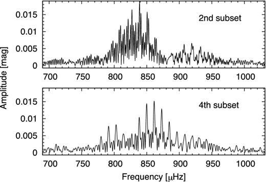
Comparison of the frequency content of the second and fourth subsets. The frequency content of GD 154 and especially the amplitudes changed from 3803 to 3847 BJD.
At first sight the Fourier spectrum of the second and fourth subsets (upper and lower panels of Fig. 5) suggests that the frequency content of GD 154 and especially the amplitudes changed from 3803 to 3847 BJD.
We clearly recognize distinct peaks at 839 and 918 μHz in the second subset and at 861 and 802 μHz in the fourth subset. The accepted frequency content of the two subsets as a result of comparative analyses is given in Table 2. We found a doublet around the dominant mode in the second subset and four doublets in the fourth subset, for a total of five and nine frequencies, respectively. The triplets are not resolved on the subsets. Although the frequency values obtained on the different data sets agreed within 1 μHz in most cases, the amplitudes are remarkably different at different epochs.
3.2.1 Results on data simulation
Two points were checked in synthetic data. The frequency spacings of 839.14 and 883.56 μHz frequencies to the newly found mode at 861.56 μHz are 22.42 and 22.0 μHz, about twice the daily alias pattern (11.57 μHz), which could be confusing in the case of a single-site observation. The reason of the apparently variable amplitudes of the 839.14 and 861.56 μHz frequencies in the two subsets was also checked, whether they are interaction of the unresolved triplets or they represent intrinsic amplitude variation of normal modes.
Synthetic data were generated with the different combination of the possible normal modes, doublets and triplets, with constant amplitude for the time series of the whole season and the two subsets. The analyses of the synthetic data were conclusive.
The five possible normal modes can be obtained with high precision not only for the whole data set but for the subsets, too. We confirmed that the new frequency at 861.56 μHz is a real normal mode; it cannot appear by the daily alias interaction. The interaction of doublets does not cause large amplitude changes in the subsets. The interaction of the three triplets on shorter timebase can cause as large amplitude increase as the one we found in the analyses of our real time series. However, the amplitude ratio of the 838.92 and 861.52 μHz frequencies did not change in the synthetic data. The amplitude of the 838.92 μHz frequency was always higher in both subsets than the amplitude of the 861.56 μHz frequency. We confirmed that both modes reveal real amplitude variations over a 50 d time-scale. As we require a stable frequency solution for our single-site measurements, we present a solution that includes only the doublets.
3.2.2 Harmonics and subharmonics
We performed frequency analyses in the region of harmonics and subharmonics, too. An independent frequency at 2484.14 μHz was definitely found on those nights when the star showed multimode pulsation.
We found groups of peaks around 1652.78, 1711.81, 1752.31 and 1836.81 μHz values but they do not correspond exactly to twice the value of the mother frequencies and it is difficult to explain them as linear combinations. However, the second harmonic of the dominant mode (2517.48 μHz, the mother frequency is 839.14 μHz), near to the high-frequency independent mode (2484.14 μHz), was clearly recognized.
Linear combinations of the dominant mode and its doublet with the high-frequency independent mode were detected at 3253.47 and 4155.09 μHz. Although these values are near the 4F and 5F values, they agree with the linear combination explanation much better.
On the last, but unfortunately the shortest nights only a single mode at 842.93 μHz seems to be excited, instead of a multimode behaviour. It corresponds to the rotational component (at 843.15 μHz) that was dominant in the discovery and the WET runs. In Fig. 6, we present the light curves of the fifth subset (BJD 3930–3936) folded by the dominant mode of the subset, 842.93 μHz (upper panel), and by the actual value of the dominant mode of the whole data set, 838.94 μHz (lower panel). The narrow spread of the measurements in the upper panel proves that the star has a single mode dominant and this dominant mode is 842.93 μHz in the BJD 3930–3936 interval. Unfortunately, we could not follow in details this status of the pulsation that seems to appear from time to time between the multimode states. On 2007 April 20 and 21, GD 154 showed a pure monoperiodic pulsation state (Montgomery, private communication) with harmonics and subharmonics. The convective response time-scale of the DAV star EC14012−1446 was compared partly to that value of GD 154 obtained from the monoperiodic light curves (Provencal et al. 2012). Weak signs of the subharmonics (at 1195.60 and 1291.67 μHz) appeared mostly on our last short nights connected to the single-mode pulsation. There were nights when the sign of the 2.5 times (2104.17 μHz) or 3.5 times (3003.47 μHz) values of the mother frequency could also be found.
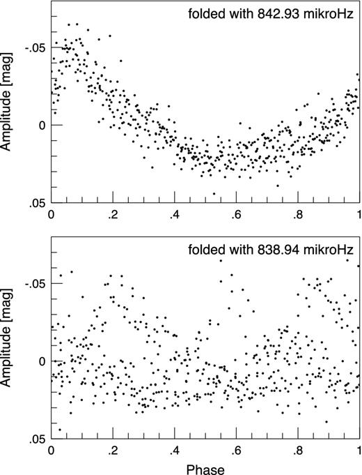
The light curves of the fifth subset (BJD 3930–3936) folded by the dominant mode of the subset (upper panel) and by the dominant mode of the whole data set (lower panel). The regular arrangement of the upper panel suggests a monoperiodic pulsational phase of GD 154 during the given interval.
The Fourier parameters of the final accepted frequency content of GD 154 are given in Table 3.
The frequency content of GD 154 at 2006. Four doublets and two independent modes were found. The modes at 861.56 and 807.62 μHz have never been reported before.
| Freq. | Period | Ampl. | Phase |
|---|---|---|---|
| (μHz) | (s) | (mmag) | (°) |
| 839.14 | 1191.7 | 8.38 | 314.4 |
| 843.15 | 1186.0 | 6.90 | 1.9 |
| 861.56 | 1160.7 | 5.76 | 276.5 |
| 864.55 | 1156.7 | 4.91 | 152.8 |
| 918.70 | 1088.5 | 4.44 | 215.6 |
| 921.61 | 1085.1 | 3.88 | 94.6 |
| 807.62 | 1238.2 | 4.64 | 218.9 |
| 803.74 | 1244.2 | 4.38 | 144.0 |
| 883.56 | 1131.8 | 4.12 | 337.4 |
| 2484.14 | 402.6 | 3.50 | 82.6 |
3.2.3 Characteristic features in the light curves
A fit, generated by the Fourier parameters given in Table 3, describes the general features of the light curve of GD 154. However, there are intervals containing some (4–6) cycles where the measurements represent much higher amplitudes for the cycles than the fit. Two special features were isolated. In panel (a) of Fig. 7, the envelope of the measurements resembles a Gaussian profile with a steep increase before the maximum and a steep decrease after it. The fit by our mode decomposition gives a much lower regular amplitude of the cycles. Both the solution (only the modes in the 760–960 μHz interval) for the whole data set (continuous line) and the separate solution for the fourth subset (dotted line) are compared. The latter slightly increased the amplitude of the fit, but in the maximum-amplitude cycle only about 50 per cent of the amplitude is covered by the fit. Similar high-amplitude intervals are between BJD 3803.34–3803.44 and 3850.46–3850.56. The inclusion of the rotationally split components helped to increase the amplitude but it was still not enough to match the observed amplitude. It is difficult to imagine such a missing pulsation mode that could help to fit the high-amplitude cycles without destroying the acceptable fit of the low-amplitude cycles. It is more probable that some additional physical process is superimposed on the pulsation creating high-amplitude phases. Maybe we are faced with an extra effect of convection with the pulsation.
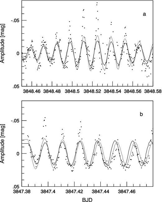
Special features in the light curves of GD 154. (a) Intervals containing 4–6 cycles where the measurements represent much higher amplitudes for the cycles than the fit (may be the interaction of the pulsation with convection). (b) Alternating high- and low-amplitude cycles follow each other (may be chaotic behaviour of the pulsation). Fits for the solution for the whole data set (continuous line) and for the fourth subset (dotted line) are also given.
A second characteristic feature is presented in panel (b) of Fig. 7: alternating high- and low-amplitude cycles follow each other. Neither the frequency solution of the whole data set nor the fourth subset can fit the light curve of these cycles. Similar features can be found between BJD 3847.51–3847.56, 3851.48–3851.54 and 3935.34–3935.39. The presented case in panel (b) shows a phase shift between the solution for the whole data set and the fourth subset. The alternating high- and low-amplitude cycles remind us of the chaotic behaviour of the stellar pulsation.
3.3 Rotational splitting
Thanks to regular observations over the whole season, we could find not only the normal modes but members of rotationally split frequencies. The direct determinations of the rotational splittings are 4.01, 2.99, 2.91 and 3.88 μHz for the doublets presented in Table 3, respectively. Considering the three triplets listed in Table 2, we recognize that they are asymmetrically spaced and the m = 0 to +1 splits are always smaller. This suggests that the ≈ 920 μHz doublet peaks, as also having small spacing, belong to m = 0 and +1 modes.
We use the term ‘triplets’ for the multiplets we found, but without any mode identification, we cannot say which ones are real triplets (dipole modes) or three of five possible components of quadrupole modes. The asymmetric structure of these closely spaced modes also makes it difficult to distinguish between the l = 1 and 2 ones. Assuming solid body rotation and that the triplet components around the dominant mode are high-overtone (k ≫ 1) l = 1 that we calculated from the 2.76 μHz average split value, the rotational period of the star is 2.1 d.
Pfeiffer et al. (1996) determined Prot = 2.3 ± 0.3 d, also derived from an asymmetric triplet with 〈δf〉 = 2.5 μHz. This rotation period agrees with our result within 1σ. Hürkal et al. (2005) found ≈3 μHz frequency splittings (〈δf〉 = 3.27 μHz), corresponding to Prot = 1.8 d. Regarding that at each epoch different frequency content was determined, the similar frequency spacings of the multiplets suggest that they really correspond to stellar rotation at a constant rate.
Besides the direct determinations, we searched for characteristic frequency spacing values applying a more sophisticated method. We selected the five main frequencies in the 65–85 d−1 range and – during a pre-whitening process – the highest amplitude ones in their vicinity. Then we performed the Fourier analysis of the frequencies obtained in this way. That is we searched for regular spacing value(s) between the frequencies which may correspond to the rotational splitting phenomenon. To check our findings, we analysed not only the whole frequency list, but some subsets of the frequencies, too. Our results suggest characteristic spacing values to be around 2.6 and 3.7 μHz (Bognár & Paparó 2013). These values are also close to the directly determined and the previously detected ones.
4 INVESTIGATION OF THE MAIN STELLAR PARAMETERS
The efforts to determine the precise frequencies of the independent modes were aimed at investigating the interior structure of the star. Asteroseismology gives us the opportunity to provide constraints on the structure of the core, the hydrogen/helium layers, the mass of the star and to estimate the star's distance. For this purpose, we ran the White Dwarf Evolution Code (wdec) originally written by Martin Schwarzschild and modified by Kutter & Savedoff (1969), Lamb & van Horn (1975), Winget (1981), Kawaler (1986), Wood (1990), Bradley (1993), Montgomery (1998) and Bischoff-Kim, Montgomery & Winget (2008).
The wdec evolves a hot (∼100 000 K) polytrope starter model down to the temperature we require, and gives an equilibrium, thermally relaxed solution to the stellar structure. For this model, the possible pulsation periods of m = 0 are determined by solving the non-radial, adiabatic stellar pulsation equations (Unno et al. 1989). Metcalfe (2001) created an integrated form of the evolution/pulsation codes, which allow us to obtain the period values with only one command. In this way we can build model grids consisting of thousands of models in a very efficient way.
We used the equation-of-state (EOS) tables of Lamb (1974) in the core, the EOS tables of Saumon, Chabrier & van Horn (1995) in the envelope of the star, OPAL opacities updated by Iglesias & Rogers (1996) and the conductive opacities by Itoh et al. (1983, 1984). The wdec treats the convection by means of the mixing length theory of Böhm & Cassinelli (1971) using the α = 0.6 parametrization according to the model calculations of Bergeron et al. (1995). The hydrogen/helium transition zone was treated by equilibrium diffusion calculations, while the helium/carbon transition layer was parametrized.
We built two model grids using different core composition profiles. In one case, we varied five input parameters of the wdec: Teff, M*, MH, XO (central oxygen abundance) and Xfm (the fractional mass point where the oxygen abundance starts dropping) and fixed the mass of the helium layer at the 10−2 M* ‘canonical’ value. In the second scan, we varied the mass of the helium layer, but used the core profiles of Salaris et al. (1997) based on evolutionary calculations. For this second grid, only four stellar parameters were scanned. Table 4 shows the parameter space covered by our grids and the step sizes applied.
We varied the stellar parameters and built model grids according to the minima and maxima values and step sizes given in the table.
| Grid | Teff (K) | M* (M⊙) | −log MHe | −log MH | XO | Xfm |
|---|---|---|---|---|---|---|
| 1 | 10 600−11 800 | 0.600−0.800 | 2 | 4−11 | 0.5−0.9 | 0.1−0.5 |
| 2 | 10 600−11 800 | 0.600−0.800 | 2−3.5 | 4−11 | Core profiles by Salaris et al. (1997) | |
| Step sizes: | 200 | 0.005 | 0.5 | 0.2 | 0.1 | 0.1 |
The Teff and log g values of GD 154 determined by high signal-to-noise optical spectrophotometry are 11 180 K and 8.15 dex, respectively (Bergeron et al. 1995). Considering that the external uncertainties are estimated to be hundreds of kelvins and could achieve ±0.1 dex, we decided to cover a relatively large range in effective temperature and surface gravity. A DA white dwarf with log g = 8.15 has a mass of ∼0.7 M⊙. In our grids, we searched for the best-fitting models in the range log g ∼ 8.0–8.3 (0.6–0.8 M⊙; see the tables of Bradley 1996). Bergeron et al. (2004) estimated ∼200 K and ∼0.05 dex for the external errors of Teff and log g, respectively. According to these values, our grid covers a ±3σ range in Teff and M*.
Pfeiffer et al. (1996) suggested a very thin hydrogen layer for GD 154 with the mass of 2(±1) × 10−10 M*. Taking their result into account, we allowed for hydrogen layer masses between 10−4 and 10−11 M* in the grids.
We also used the data base of ZZ Ceti periods (dipole and quadrupole) calculated from fully evolutionary models (Romero et al. 2012a). The period values were derived by models with consistent chemical profiles from the core to the surface. The authors allowed the evolution of the stars from the zero-age main sequence in the calculations of these profiles. More details on the code, the input physics and a number of examples of its asteroseismological applications can be found in Althaus et al. (2010) and Romero et al. (2012b).
4.1 Parameters of the best-fitting models
We used two slightly different sets of periods for the asteroseismological investigations of the star. Our frequency analyses and tests show that the periods given in Table 3 describe the light variations of GD 154 in the 2006 observational season well. Accordingly, the values used in our first run are 402.6, 1088.5, 1131.8, 1160.7, 1191.7 and 1238.2 s, respectively. The second run differs from this in one period only: we replaced the 1191.7 s mode with 1186 s, the one with the second largest amplitude. During the 1991 WET observations, the period of the dominant mode was 1186.5 s and was found to be the m = 0 component of an (asymmetric) triplet (Pfeiffer et al. 1996). As Tables 2 and 3 show in our data set, the 1191.7 s period dominates. This one is still part of a triplet structure and could be regarded as the m = −1 peak of the 1186 s mode. We used two different sets of periods because of this ambiguity. In this way, we could examine the effect of slightly different periods on the best-fitting models’ parameters.
Even though we doubled the number of known period values applied in the star's seismic investigations compared to previous research, GD 154 is still not a pulsator rich in known modes. This means that we find several models with low σrms values as the result of the fitting procedure. Therefore, we applied further constraints during the model selection: assuming better visibility of l = 1 modes, we selected the models with at least three l = 1 solutions to the observed periods. As an additional criterion, we considered the ones which give the l = 1 value for the dominant (1186 or 1191.7 s) mode. However, as the average period spacing of the long-period modes is low (below 40 s), we assumed that the observed modes are not solely l = 1 ones, because this would require a much higher stellar mass for GD 154 than the spectroscopic value.
4.1.1 Stellar parameters
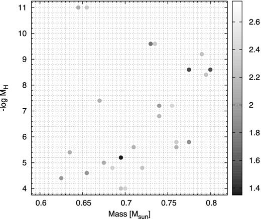
The left-hand panel of Fig. 8 shows the 6 + 6 best-fitting models in the Teff-M* plane for both period lists. The numbers indicate the models’ hydrogen layer masses and we also denoted the spectroscopic solution given by Bergeron et al. (1995) with its uncertainties. As can be seen, we find the best-matching (three) models for the spectroscopic mass using the second period list. Table 5 (rows 1–3) summarizes the parameters of these models. In two cases (M* = 0.71 and 0.73 M⊙) the mass of the hydrogen layer is around 10−6 M*, while the model star with 0.705 M⊙ has MH = 1.6 × 10⁻⁸ M*, which means a considerably thinner layer. The best-matching model to the spectroscopic parameters is the one with M* = 0.73 M⊙ and Teff = 11 200 K. In this case, the mass of the hydrogen layer is MH = 6.3 × 10⁻⁷ M*.
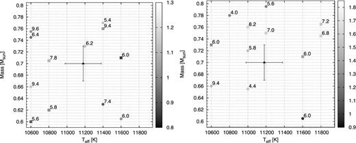
Plots of the models that best fit the data for six (left-hand panel) or seven (right-hand panel) modes in the Teff-M* plane. The circles and squares denote the solutions obtained by including the 1191.7 or 1186 s mode into the period list. Their σrms values are colour-coded. The models’ hydrogen layer masses (−logMH) and the spectroscopic solution with the corresponding uncertainties are also indicated. The background grid corresponds to our model grid's step sizes.
Parameters of the selected models using different core profiles and slightly different period values. The observed Teff and M* values (Bergeron et al. 1995) are given in the last row.
| No. | Teff | M* | −log MHe | −log MH | XO | Xfm | Period values in seconds | σrms | ||||||
|---|---|---|---|---|---|---|---|---|---|---|---|---|---|---|
| (K) | (M⊙) | (l, k) | (s) | |||||||||||
| 1 | 11 600 | 0.710 | 2.0 | 6.0 | 0.8 | 0.2 | 402.0 | 1088.9 | 1132.6 | 1159.2 | 1184.9 | 1238.4 | 0.86 | |
| (1, 7) | (1, 23) | (2, 42) | (2, 43) | (1, 25) | (2, 46) | |||||||||
| 2 | 10 800 | 0.705 | 2.0 | 7.8 | 0.6 | 0.4 | 402.9 | 1087.6 | 1131.5 | 1162.0 | 1188.1 | 1238.3 | 1.09 | |
| (2, 11) | (1, 19) | (2, 35) | (2, 36) | (1, 21) | (1, 22) | |||||||||
| 3 | 11 200 | 0.730 | 2.0 | 6.2 | 0.6 | 0.4 | 402.0 | 1090.8 | 1131.2 | 1161.3 | 1185.8 | 1239.2 | 1.13 | |
| (1, 6) | (1, 22) | (2, 40) | (2, 41) | (1, 24) | (2, 44) | |||||||||
| 4 | 11 000 | 0.720 | 2.0 | 5.8 | 0.8 | 0.5 | 400.4 | 1088.5 | 1132.2 | 1159.5 | 1194.2 | 1238.2 | 1273.4 | 1.51 |
| (1, 6) | (1, 22) | (2, 40) | (2, 41) | (1, 24) | (1, 25) | (2, 45) | ||||||||
| 5 | 11 600 | 0.710 | 2.0 | 6.0 | 0.8 | 0.2 | 402.0 | 1088.9 | 1132.6 | 1159.2 | 1184.9 | 1238.4 | 1268.5 | 1.38 |
| (1, 7) | (1, 23) | (2, 42) | (2, 43) | (1, 25) | (2, 46) | (1, 27) | ||||||||
| 6 | 11 200 | 0.675 | 2.0 | 5.2 | 0.73 | 0.54 | 402.4 | 1089.2 | 1133.6 | 1158.1 | 1191.9 | 1240.1 | 1.52 | |
| (2, 12) | (1, 22) | (2, 41) | (2, 42) | (1, 24) | (1, 25) | |||||||||
| 7 | 11 400 | 0.675 | 2.5 | 5.2 | 0.73 | 0.54 | 402.2 | 1086.5 | 1132.7 | 1160.5 | 1194.5 | 1239.4 | 1.55 | |
| (1, 6) | (1, 22) | (2, 41) | (2, 42) | (1, 24) | (2, 45) | |||||||||
| 8 | 11 000 | 0.710 | 2.0 | 5.6 | 0.73 | 0.54 | 398.9 | 1085.6 | 1131.4 | 1160.7 | 1188.0 | 1236.8 | 2.16 | |
| (1, 6) | (1, 22) | (2, 41) | (2, 42) | (1, 24) | (1, 25) | |||||||||
| 9 | 11 200 | 0.700 | 2.0 | 4.2 | 0.73 | 0.54 | 398.9 | 1085.9 | 1132.8 | 1159.9 | 1192.7 | 1236.0 | 1269.9 | 2.07 |
| (1, 7) | (2, 43) | (2, 45) | (2, 46) | (1, 27) | (1, 28) | (1,29) | ||||||||
| 10 | 11 000 | 0.710 | 2.0 | 5.6 | 0.73 | 0.54 | 398.9 | 1085.6 | 1131.4 | 1160.7 | 1188.0 | 1236.8 | 1267.7 | 2.45 |
| (1, 6) | (1, 22) | (2, 41) | (2, 42) | (1, 24) | (1, 25) | (2,46) | ||||||||
| 11 | 11 241 | 0.705 | 4.445 | 399.3 | 1082.6 | 1133.9 | 1160.0 | 1192.3 | 1239.8 | 2.97 | ||||
| (1, 7) | (2, 43) | (2, 45) | (2, 46) | (1, 27) | (1, 28) | |||||||||
| 12 | 11 639 | 0.705 | 9.339 | 404.3 | 1085.3 | 1130.7 | 1165.7 | 1182.6 | 1237.9 | 2.92 | ||||
| (1, 5) | (1, 20) | (1, 21) | (2, 38) | (1, 22) | (1, 23) | |||||||||
| Observations: | ||||||||||||||
| 11 180 | 0.70 | 402.6 | 1088.5 | 1131.8 | 1160.7 | 1191.7 | 1238.2 | 1271.5 | ||||||
| 1186.0 | ||||||||||||||
When we investigate a pulsator showing amplitude variations, it is worth checking if we can add further modes to our period lists observed in a different season. We found one mode, also presented by Hürkal et al. (2005): the one at 1271.5 s. Then we have four period lists: two with 6–6 and two with 7–7 periods. In the latter case, we selected the models with at least four l = 1 modes instead of three. As the right-hand panel of Fig. 8 shows, the parameter space occupied by the best-fitting seven-period models differs only slightly from the six-period ones. Using seven periods most of the models have M* > 0.7 M⊙. Considering the hydrogen layer masses, the average values are ∼10−7 and 4 × 10⁻⁷ M* for the six- and seven-period solutions, respectively. We can recognize in Fig. 8 that there are common models, the ones with Teff = 10 600 and 11 600 K and MH = 10−9.4 and 10−6 M*. Our best-matching models using seven periods are the 0.720 and 0.710 M⊙ ones with Teff = 11 000 and 11 600 K. They have MH = 1.6 × 10⁻⁶ and 10−6 M* (Table 5, rows 4 and 5). As can be seen, models 1 and 5 have the same parameters; this is one of the common points.
Considering the solutions with Salaris et al.'s core profiles and within the 1σ limit in M*, the hydrogen layer masses are between 10−4 and 10−6 M* in most cases and the MHe = 10−2 M* value is preferred. Rows 6–10 of Table 5 show some of their parameters; they are selected on the basis of having Teff close to the spectroscopic value. These models have MH = 6.3 × 10⁻⁵, 2.5 × 10⁻⁶ or 6.3 × 10⁻⁶ M*.
Investigating the parameters of the best-fitting models, we found a trend that more massive stellar models have a thinner hydrogen layer. An example for the phenomenon can be seen in Fig. 9, where we plotted the best-fitting models with σrms < 2.5 s in the M*-MH plane. The explanation of this phenomenon is that generally for thinner hydrogen layers, the mode trapping cycle is longer and the average period spacings between the consecutive overtone modes are also larger (i.e. there are larger differences between period spacing minima and maxima). This can be partially offset by the shorter average period spacing of a higher mass star (Bradley 1996). The panels of Fig. 10 demonstrate the influence of the varying stellar parameters on the period spectrum of a model star. The stellar mass and the mass of the hydrogen layer have a great effect on the observed periods. We can find a similar period structure for the lower stellar mass – higher hydrogen layer mass and higher stellar mass – thinner hydrogen layer models, and this results in observed trend seen in Fig. 9.
Models in the M*-MH plane with σrms < 2.5 s and Salaris et al.'s core profiles. The six-period light-curve solution with the 1186 s mode was used. The models’ σrms values are colour-coded. The background grid corresponds to our model grid's step sizes. The figure shows the trend that more massive stellar models have thinner hydrogen layer.

Period spacing diagrams of model stars with Teff = 11 200 K, MHe = 10−2 M* and 50/50 C/O fraction core. The filled and open circles denote the l = 1 and 2 modes, respectively. The panels show the influence of the stellar and hydrogen layer mass variations on the period spectrum.
Using the coarse grid of Romero et al. (2012a) we obtained the best-matching model to spectroscopy applying the first period set. It has Teff = 11 241 K, M* = 0.705 M⊙ and MH = 3.6 × 10⁻⁵ M* (Table 5, row 11). The second best-matching model belongs to the second period list and has a higher effective temperature (11 639 K) but the same mass (Table 5, row 12). The largest difference is in the mass of the hydrogen layer, which is significantly lower, only 4.6 × 10⁻¹⁰ M*. Considering all the solutions within the σrms < 3 limit, the mass of the hydrogen layer is between 3.5 × 10⁻⁵ and 7.6 × 10⁻⁵ M*, from which the latter one is the only exception.
Knowing the luminosities of the selected models, we estimated the star's asteroseismological distance by calculating the distance modulus (Bradley 2001). The log(L/L⊙) values of the models in Table 5 are between −2.7 and −2.8. The seismological distances calculated from the 10 different models of Table 5 are between 41.5 and 46.4 pc. The average distance and parallax value are 44.2 pc and 22.7 mas, respectively. This result is close to the 45.4 pc value derived by spectroscopic observations of Lajoie & Bergeron (2007), which shows that the pulsation analysis supports the spectroscopic result on the distance parameter.
For the sake of completeness, we summarized the results obtained by previous asteroseismological investigations of GD 154 in Table 6.
Physical parameters and mode-identification results presented by different authors. They selected the model solutions using the period values determined by the 1991 WET campaign (Pfeiffer et al. 1996). The atmospheric parameters and periods obtained by observations are denoted by asterisks.
| Teff (K) | M* (M⊙) | −log MHe | −log MH | Period values in seconds (l, k) | Ref. | ||
|---|---|---|---|---|---|---|---|
| 11 180* | 0.7* | 9.7 | 402.6*(1) | 1088.6*(2) | 1186.5*(1) | Pfeiffer et al. (1996) | |
| 11 200 | 0.68 | 2.0 | 7.5 | 398.2(1, 5) | 1088.5(1, 19) | 1186.9(1, 21) | Castanheira & Kepler (2009) |
| 10 800 | 0.73 | 2.5 | 9.5 | 396.9(1, 4) | 1088.5(1, 18) | 1186.5(1, 20) | Castanheira & Kepler (2009) |
| 11 574 | 0.705 | 2.1 | 9.3 | 405.0(1, 5) | 1088.9(1, 20) | 1186.6(1, 22) | Romero et al. (2012b) |
4.1.2 Mode identification
As was already mentioned, we placed a constraint only on the l value of the dominant mode: we assumed that it is l = 1. All of the other modes were allowed to be l = 1 or 2. Considering the l and k values of the selected models in Table 5, we obtained the same l only in the case of the 1160 s mode. This result suggests that it may be l = 2. None of the selected models gives l = 1 solutions for all of the periods. We cannot uniquely assign an l value for the other modes; however, the 402, 1088 and 1131 s modes’ l values are 1, 1 and 2, respectively, in the vast majority of cases. Assuming that the 1131 and 1160 s modes are l = 2, they represent consecutive overtones.
The models selected by Castanheira & Kepler (2009) and Romero et al. (2012b) (see Table 6) give l = 1 solutions for the 402, 1088 and 1186 s modes as well.
4.1.3 Mode trapping and the mass of the hydrogen layer
Pfeiffer et al. (1996) assumed that mode trapping – as an efficient mode selection mechanism – could be responsible for the small number of observed modes in GD 154 and determined a very low mass for the hydrogen layer (∼10−10 M*). As Table 6 shows, the results of the previous asteroseismological investigations also supported the presence of a very thin hydrogen layer. However, considering our selected models in Table 5, we found that the masses of hydrogen layers were higher than expected. Our model solutions have MH values between 6.3 × 10⁻⁵ and 6.3 × 10⁻⁷ M* (with an average value of 3.9 × 10⁻⁶) except for two cases, when MH = 1.6 × 10⁻⁸ and 4.6 × 10⁻¹⁰ M*. However, these latter models are below or above the 1σ limit in effective temperature. Our results show that although GD 154 may have a thinner hydrogen layer than the maximum allowed (MH ≈ 10−4), no extremely thin layer is necessary to explain the sequence of the observed periods.
The question is raised: why the other authors obtained lower mass values for the hydrogen layer. The answer may be the number of modes used in the period fits. Both Castanheira & Kepler (2009) and Romero et al. (2012b) worked with the three periods determined by Pfeiffer et al. (1996). This fact obviously strongly influenced the outcome of the fit. The results of Pfeiffer et al. (1996) have not been obtained by performing period fits with a model grid. Because of the small number of known modes, they needed to impose further constraints. As mode trapping means an efficient mode selection mechanism, they assumed that the observed modes are trapped in the outer hydrogen layer and derived the MH ≈ 10−10 M* value. In our case, the increased number of observed modes is sufficient for the asteroseismic investigations using model grids, including searching for trapped modes among the observed ones.
We constructed the (forward) period spacing diagrams for our selected models (Fig. 11). Minima in the diagrams denote departures from the uniform period spacings caused by mode trapping (see e.g. Bradley & Winget 1991). Fig. 11 shows that the long-period modes do not show tendency to occur around minima, so our model selection does not support the idea of mode trapping at long periods as a mode selection mechanism. The best candidate for a trapped mode is the 1238 s one according to Fig. 11. However, the situation is different in the case of the only short-period mode. In most cases, we can find it near or at a period spacing minimum. This suggests that the 402 s mode could be a trapped mode.
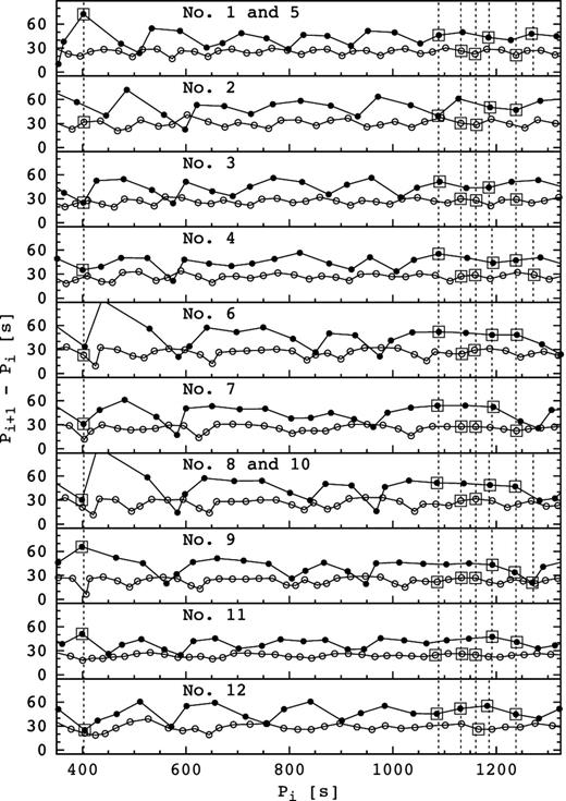
Period spacing diagrams of the 10 different models of Table 5. The filled and open circles denote the l = 1 and 2 modes, respectively. The vertical dashed lines mark the observed period values. We denoted the periods analogous to the observed ones in the given model with open squares. The models’ numbers corresponding to Table 5 are also indicated in the panels.
5 SUMMARY AND CONCLUSIONS
Our comparative period search confirmed the frequencies found previously, except the one at 787 μHz given by Hürkal et al. (2005). Additionally, we localized modes at 807.62 and 861.56 μHz values that have never been reported before. We confirmed by test investigations that six modes can be considered as independent normal modes of pulsation.
Four doublets around the largest amplitude modes were directly found. The dominant mode of our whole data set (839.14 μHz) and the dominant mode observed in two previous pulsation stages (843.15 μHz) are members of the same rotational triplet. This latest member of the triplet became dominant at the end of our observing run, when GD 154 also presented a monoperiodic pulsational stage.
We localized the second harmonic of the mother frequency at 2517.48 μHz, near the high-frequency normal mode at 2484.14 μHz, and some linear combinations too. However, no subharmonics reported by previous observations were found over our whole observational season. Characteristic features are localized in the light curves partly suggesting an effect of convection on the pulsation and reminding us of the chaotic behaviour of stellar pulsation.
Comparative analyses of subsets revealed and test investigations confirmed a remarkable intrinsic amplitude change of frequencies at 839.14 and 861.56 μHz, although part of it can be caused by unresolved rotational triplets.
With our new frequencies we have doubled the number of period values applied in the star's previous seismic investigations, which allows a more detailed study of GD 154. We found models with effective temperatures and masses within the 1σ limit of the spectroscopic values (≈11 000–11 400 K and 0.68–0.73 M*) that fit the observed periods well and also give l = 1 solutions for at least half of the modes. The best-fitting models have hydrogen layer masses between 6.3 × 10⁻⁵ and 6.3 × 10⁻⁷ M*, which suggests orders of magnitude thicker layer than previously published. The explanation of this difference may be the number of modes used for the seismic studies and that we did not assume that our observed modes were trapped ones. Considering the mass of the helium layer, our results also support the 10−2 MHe ‘canonical’ value.
The known luminosities of our selected models allowed us to determine the seismic distance of GD 154. In agreement with other authors’ finding, the average value calculated by our selected models is 44 pc. We also investigated the possibility of mode trapping, constructing period spacing diagrams. Our results do not support the idea of mode trapping at long periods as a mode selection mechanism, and suggest that the short-period mode may be a real trapped mode. This result shows that we do not have to presume that all the observed modes are trapped ones.
For altering pulsation between the multi- and monoperiodic stage and the requirement for more constraints for modelling, further investigation of the complex behaviour of GD 154 is needed. Regular monitoring of the star would be necessary not only to detect new pulsation modes for asteroseismic investigations but also to follow up more mono- and multiperiodic stages. This might allow us to determine whether this altering between the two pulsation stages has any regular behaviour.
The authors thank Agnès Bischoff-Kim for providing her version of the wdec and the fitper program. The authors also acknowledge the contribution of P. I. Pápics, E. Bokor, Gy. Kerekes, A. Már and N. Sztankó to the observations of GD 154.
iraf is distributed by the National Optical Astronomy Observatories, which are operated by the Association of Universities for Research in Astronomy, Inc., under cooperative agreement with the National Science Foundation.
