


Abstract
The light curves of mutual eclipses and occultations between the natural satellites of a planet allow us to obtain high-precision position and relative motion from differential photometry, enough to detect weak orbital disturbing forces, such as tidal forces. The observations are made during the equinoxes of the planet.
We studied 25 light curves observed in Brazil during the 2009 campaign of the Galilean satellites’ mutual phenomena. A narrow-band filter centred at 890 nm was used, strongly attenuating the Jupiter's scattered light. We fitted the occultation and eclipse light curves using semi-analytical models that take into account the gradual decrease of light over the shadow, the solar limb darkening and the solar phase angle. The Oren–Nayar reflexive model was used to map the inhomogeneous light scattering on the surface of the satellites. For the first time it is used in a work about mutual events. Here, we include the study that made us decide for this model.
We measured the impact parameter, relative velocity and central instant with average precisions of 7.46 km (2.2 mas), 0.08 km s−1 (0.02 mas s−1) and 0.42 s (6.13 km), respectively. The fit precision of the normalized light-curve fluxes ranged between 0.4 and 4.4 per cent.
1 INTRODUCTION
A thorough study of the nature of the giant planet systems involves a refined comprehension of the dynamic evolution of their satellites. This requires the use of more sophisticated orbital evolution models, that take into account very weak disturbing forces, such as tidal forces, for example. In turn, the study of such models demands cinematic data bases (positions, velocities), which should cover large periods of time and should contain highly accurate astrometric measurements of the satellites (Aksnes & Franklin 2001; Vienne 2008; Lainey et al. 2009).
In this context, the photometric observations of mutual phenomena have an important advantage over traditional astrometric observations. Although such observations can only be done from time to time, during the equinox of the planet, they provide much better precisions. Indeed, for the Galilean satellites, the precision obtained with the current astrometric techniques, for a single satellite position, ranges between 134 and 170 mas (milliarcsecond) (Kiseleva et al. 2008). For relative distances between satellite pairs, the 30 mas error level can be achieved (Peng et al. 2012). On the other hand, for past mutual phenomena, the errors can easily reach the 20–30 mas range, and many times not exceed 5 mas (Emelyanov 2009). In this work, the average precision was even better, 3.10 mas.
Mutual phenomena between the Jovian satellites were observed for the first time in 1973 (Aksnes & Franklin 1976), and again in 1979, followed by the observation of the mutual events of the Saturnian satellites in 1979–1980 (Aksnes et al. 1984). A detailed history of all the past campaigns of mutual events between the satellites of the giant planets, as well as a compilation of past reduction methods and recent improvements in the fit of light curves can be seen in Emelyanov (2009) and in the references therein.
Because of the importance of mutual phenomena, many researchers have worked in their prediction and organized observational campaigns to study both of these systems (see Aksnes & Franklin 1990; Thuillot & Arlot 1996; Arlot, Lainey & Thuillot 2006; Arlot & Thuillot 2006 for the more recent works). In 2007, mutual phenomena between the Uranian satellites were observed for the first time with CCD technology (since they occur every 42 yr), and provided important astrometric results (see, for example Birlan et al. 2008; Assafin et al. 2009 and Christou et al. 2009).
Based on the prediction of the events between the Galilean satellites for 2009 (Arlot 2008), a Brazilian campaign was organized, involving researchers from four institutes. Observations were carried out at the Observatório do Pico dos Dias (OPD), managed by the Laboratório Nacional de Astrofísica (LNA), Itajubá, Brazil (IAU code 874). We successfully observed and analysed 25 events (13 occultations and 12 eclipses). Here, we present the observational procedures, the data reduction and the analysis of these events.
In Section 2, we describe the campaign's programme and observations. In Section 3, we present the photometry and the light-curve fitting procedure, with a complete description of the analytical models used. We give the results in Section 4. Section 5 brings a discussion about the available light reflectance models, and the introduction of the Oren–Nayar's model, adopted in this work. Conclusions are set in Section 6. In Appendices A and B, we detail the calculations involved in the light-curve fits, related to the adopted analytical models. In Appendix C, we display the fits to the entire set of 25 light curves analysed in this work.
2 PROGRAMME AND OBSERVATIONS
2.1 Programme
The observational campaign in Brazil was the result of a collaboration between four national institutes. The predicted events for 2009–2010 (Arlot 2008) were available at the portal of the ‘Institut de Mécanique Céleste et de Calcul des Éphémérides’ (IMCCE)1 from the Observatoire de Paris. We selected all the visible events for the OPD/LNA observatory2 with a predicted non-zero flux drop and elevation above 30 degrees. This resulted in 50 events distributed in 45 nights spread over nine months. We attempted observations for all these events.
2.2 Observations
We lost 23 events due to bad weather conditions. Also, from the remaining 27 mutual phenomena successfully observed in 23 nights, two were quasi-simultaneous, superposed in the same light curve. These two events will not be studied in this work. The resulting 25 events analysed in this work are divided into 12 eclipses and 13 occultations. The satellites Io, Europa and Ganymede were all eventually observed in an occultation or in an eclipse and Callisto was observed only in eclipses.
The events were observed at the OPD/LNA (λ = +450 32′ 57′′, ϕ = −220 32′ 22′′, h =1860 m, IAU code = 874). The observations were carried out using the 0.6 m diameter Zeiss telescope, f/12.5. For one night (20/06), the 1.6 m diameter Perkim–Elmer telescope, f/10, was used.
Owing to methane in the Jupiter's atmosphere, the planet has a strong absorption of light between 880 and 900 nm, which causes the planet albedo to drop to 0.1 in this region (Karkoschka 1994, 1998). As it does not occur with the satellites, a narrow-band filter at these wavelengths was used to strongly minimize the scattered light of Jupiter. The effect is shown in Fig. 1. The planet and its satellites present about the same brightness. This ‘methane’ filter is centred at 890 nm with a bandwidth of 20 nm.
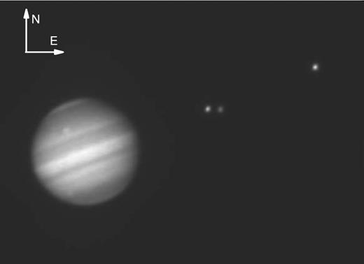
Image of Jupiter, Io, Europa and Calisto (left to right) obtained with the 0.6 m diameter Zeiss telescope, equipped with a methane filter. The planet and the satellites present about the same brightness. Due to the use of this filter, centred at λ = 890 nm with 20 nm width, the scattered light from Jupiter is severely minimized.
We used two back illuminated CCD detectors. The EEVCCD detector (model 02-06-1-206) with 385 × 578 square pixels of 22 μm, hereafter CCD 301, was used in 23 out of the 25 events studied in this work. The EDVCCD detector (model 47-20) with 1024 × 1024 pixels of 13.5 μm was used in the two events observed at the Perkim-Elmer telescope (2006CeI-1 and 2006CeI-2, see Table 1). Since mutual phenomena are short-term events (typically a few minutes long) with relative satellite velocities above 6 km s−1, they demand short exposures for achieving a time resolution corresponding to a spatial resolution of a few kilometres. In practice, depending on the specific relative speed and on the weather conditions, the exposure times ranged between 1 and 3 s. This granted satellite's ADU (analogic-to-digital unit) peak counts of about half the CCD maximum, allowing for high signal-to-noise ratios (S/N) at the optimal linear count ranges of the CCDs. The electronics of the detectors were set to do simultaneous integration and charge transfer (frame-transfer mode), eliminating the readout overhead between acquisitions.
Observations were made in order to always keep the same photometric calibrator in the field of view (FOV). In eclipses, sometimes the eclipsing satellite was the calibrator. In the absence of suitable satellites, Jupiter – and sometimes a spot on its surface – was used instead. Yet, due to the large separation of the targets, two events were observed without a calibrator: an occultation of Io by Europa on August 07 and an occultation of Ganymede by Europa on August 12.
The FOV was 4 arcmin × 4 arcmin, with a pixel of 0.6 arcsec size. Seeing was typically in the range 1–2 arcsec.
Observations started 30 min before and ended 30 min after the predicted instants provided, respectively, for the start and end of the event. This procedure aimed to obtain well resolved images of the satellites involved, with enough angular separation to measure their individual fluxes, as close as possible to the event, to determine the ratio of albedos (see discussion in Section 3.2).
Table 1 gives information for the 25 events analysed in this work, indicating the targets, calibration object, seeing, zenith distance, number of images and solar phase angle.
Mutual events and observation conditions.
| Date | Event | Cal. | Seeing | No. of | z | Solar |
|---|---|---|---|---|---|---|
| (d-month) | (arcsec) | images | (°) | phase (°) | ||
| 27-04 | 2704GoI | E | 2.3 | 1800 | 52.69 | 10.97 |
| 09-05 | 0905EoI | C | 1.7 | 1401 | 34.26 | 11.41 |
| 21-05 | 2105IoE | G | 1.9 | 1302 | 53.31 | 11.48 |
| 28-05 | 2805IoE | G | 1.9 | 802 | 14.70 | 11.33 |
| 10-06 | 1006GeC | G | 2.0 | 1301 | 9.81 | 10.64 |
| 16-06 | 1606GeI | G, E | 1.8 | 2701 | 22.54 | 10.18 |
| 19-06 | 1906CeE | C | 2.1 | 1201 | 29.21 | 9.90 |
| 19-06 | 1906CeI | C, E | 1.6 | 1201 | 22.12 | 9.89 |
| 20-06 | 2006CeI-1 | S | 1.2 | 2500 | 28.89 | 9.80 |
| 20-06 | 2006CeI-2 | C | 1.7 | 2273 | 28.65 | 9.78 |
| 22-06 | 2206IoE | J | 1.2 | 2500 | 50.29 | 9.59 |
| 29-06 | 2906IoE | J | 2.2 | 1000 | 14.83 | 8.73 |
| 04-07 | 0407IeG | J | 2.2 | 1801 | 9.85 | 8.02 |
| 06-07 | 0607IeE | I | 1.9 | 2000 | 9.9 | 7.72 |
| 06_07 | 0607IoE | J | 1.9 | 1200 | 27.54 | 7.71 |
| 08-07 | 0807GeI | G, E | 1.8 | 1800 | 39.05 | 7.40 |
| 13-07 | 1307IeE | E | 1.9 | 2000 | 40.75 | 6.56 |
| 07-08 | 0708IeE | S | 2.0 | 1800 | 23.67 | 1.64 |
| 07-08 | 0708IoE | N | 2.0 | 1700 | 28.82 | 1.64 |
| 12-08 | 1208GoE | N | 2.4 | 1400 | 7.45 | 0.63 |
| 22-08 | 2208IoE | J | 2.4 | 2500 | 23.33 | 1.62 |
| 16-09 | 1609IoE | J | 2.5 | 1400 | 6.15 | 6.57 |
| 16-09 | 1609IeE | I | 2.0 | 1100 | 22.19 | 6.57 |
| 24-10 | 2410GoE | I | 3.8 | 2600 | 34.33 | 10.94 |
| 25-10 | 2510IoE | J | 3.8 | 600 | 45.96 | 10.98 |
Note. All observations were made in 2009. For each event, we have the day and month, the target satellites designated by their initials (capital letters), and the event type (‘e’ and ‘o’ stand for eclipse and occultation, respectively). Also indicated are the objects used as calibrators (Cal.) in the differential photometry: J stands for Jupiter, S for a spot on Jupiter and N means no calibrator available. We also give the seeing, the total number of images used, the zenith distance z and the solar phase angle. There was no prediction in (Arlot 2008) for the event 1208GoE.
3 PHOTOMETRY, LIGHT-CURVE FITTING
In this section, we will describe: (a) the differential aperture photometry applied to generate the observed light curves; (b) the technique used for determining the ratio of albedos; (c) the analytic models and numerical computations utilized to fit the observed light curves.
3.1 Photometry
All images were corrected by bias and flat-field using the iraf package (Butcher & Stevens 1981). Differential aperture photometry was performed using the praia package described in Assafin et al. (2009). The flux of the target was measured relative to a calibrator, usually another satellite or satellites, sometimes the eclipsing one (in eclipses). The resulting measured target/calibrator flux ratio is practically free from the sky transparency variations owing to anomalous atmospheric extinction, as this affects all objects in almost the same manner in the FOV. The S/N, the flux ratio error and the seeing are calculated and stored together with the mid-time instant of the measurements. After measuring the flux ratio for all the images, we obtained the observed light curve of the event.
In order to maximize the S/N, for each event we tested the optimum size of the aperture radius for the flux determination of each object, and for the sky background annulus. We varied their sizes for each series of observations, and plotted the resulting sets of provisional light curves. We choose the aperture values and sky background annulus which resulted in the light curve with the least flux dispersion. Typically, the sky background annulus around the objects had an internal radius 5 pixels larger than that of the aperture circle, and a width of 5 pixels. We did not verify a clear linear relation between the best aperture radius size and the seeing of the night for the events of this campaign.
From Table 1, we notice that for some events, Jupiter or a spot on its surface were used as calibrator. We verified the validity of such calibrators by comparing the light curve of an event that had a satellite as calibrator, with the light curve of the same event obtained with Jupiter or a spot as the calibration object. Although we add a certain amount of noise in the flux ratio, the procedure proved to be effective.
In two cases, no calibrator at all was available in the FOV. For these events, we fitted a polynomial to the light curve outside the flux drop, and flatted the entire curve to eliminate the continuous variation of the flux, due to the atmospheric extinction. The procedure proved to be satisfactory, since the sky conditions were very stable. In both cases, the light curves were thus directly obtained from the fluxes of the targets.
As a final step, all observed light curves were normalized by fitting a polynomial curve of nth degree (usually n = 1) outside the flux drop, so that the flux ratio was set to 1 outside the events.
3.2 Ratio of albedos
The ratio of albedos is not relevant for eclipses when the satellites’ photometric fluxes are separately measured, as is our case. Therefore, the following discussion concerns only to occultations.
The ratio of albedos is a physical parameter that is related to the reflectivity of the satellites. Since the albedo is the ratio between the received and reflected light by the satellites, the ratio of albedos has great influence on the flux ratio shape of the light curve of an occultation. In particular, it has a high correlation with the impact parameter, which is the minimum distance at apparent closest approach. Because of this correlation, it is highly recommended that we determine the ratio of albedos independently from the reduction process, instead of trying to fit it from the light curve, together with the other parameters.
There are maps of albedos for the Galilean satellites provided by the Voyager and Galileo probes (see, for example, Vasundhara et al. 2003). But they were not generated in the same bandpass (filter) as our observations. And there is no reliable process to convert these albedos to our methane bandpass, or to other wavelengths, because of photoclinometry effects, such as shadows cast by the relief at the time of the probe's measurements, which are not present in the ground-based observations, and vice-versa.
3.3 Light-curve fitting procedure
We rigorously reproduced the geometry of the mutual events by formulating theoretical models and performing numerical computations. We then could determine the apparent configuration of the satellites and of the Sun (including shadows), and thus be able to infer the amount of light received by the observer at any instant. This flux in turn was compared and fitted to the observed light curves in an iterative procedure. As a result, we determined the observed apparent relative orbital paths of the target satellites, described in terms of known parameters: the impact parameter (the minimum apparent distance between the geometric centre of the satellites, at the apparent closest approach in the sky plane), the relative velocity (tangent to the point associated with the impact parameter, measured in the sky plane) and the central instant (instant of time associated with the impact parameter). It is important to emphasize that the impact parameter is defined by using the geometric centre of the satellites which, unlike the photocentre, do not depend on the solar phase angle. The satellites’ ephemeris can also be represented by these parameters, so that we could compare the results from the observations with the current established ephemeris for the Galilean satellites.
We assume an apparent linear path for the relative motion between the target satellites, during the short time interval of the events. We model the light curves of the events based on a rigorous formulation of the geometry of the relative orbits and of the effects of light reflectance over the satellites’ surfaces. The normalized flux ratio cannot be directly expressed in terms of a simple analytical function. For each instant of observation, we calculate the flux by numerically simulating the two-dimensional luminosity profile of the satellites’ discs, projected on to the sky plane perpendicular to the line of sight. These profiles depend on the type of the event (occultation or eclipse), and on the positions of the satellites and of the Sun. As a result, we derive a simulated light curve, which works as the model. This light curve is parametrized by the relative orbital parameters described above. The observed light curve is then fitted to this simulated light-curve model by an iterative non-linear least-squares procedure, which follows the Levenberg–Marquardt method. The derivatives of the simulated light-curve model with respect to the orbital parameters are numerically computed by varying the parameters. In the process, as the flux of the simulated light-curve model converges to the flux of the observed light curve, so do the values of the orbital parameters being adjusted. After a convergence of 1 per cent is reached in the chi-square (flux) between the simulated and observed light curves, we obtain the desired orbital parameters. The spatial resolution of the luminosity profile is set (limited) by the time resolution and photometric measuring errors of the observations, thus at the same time avoiding loss of precision, and optimizing computation speed. Typically, we used resolutions corresponding to 10 × 10 km areas in the sky plane.
We fit the projected relative velocity, the central instant, and the impact parameter with this procedure. Initial guess values for these parameters are necessary to start the procedure. They are solely obtained from the observed light curve itself, which makes the process ephemeris independent. On the other hand, we use the formalism above to rigorously compute relative velocity, central instant and impact parameter, based on a given ephemeris. This translation allows for a direct and unbiased comparison between the ephemeris-based and the fitted parameters, which model the observed light curves of the mutual events (see Section 3.4).
The initial guess values are calculated from the observed light curve as follows. The central instant is obtained from the instant associated with the observation with minimum flux. The relative velocity is computed by considering the diameter of the occulted/eclipsed body and the time interval from ingress to egress, estimated from the observed light curve. The impact parameter is derived in an iterative process. We increment the impact parameter values from zero to a given limit, which is the sum of both satellites’ radius for occultations, or the penumbra size plus the radius of the eclipsing satellite, in the case of eclipses. For each incremented value, we compute the simulated flux associated with the estimated central instant and to four other points, uniformly located between ingress and egress. Then, we store the chi-square, which is the square root of the ratio between the sum of the differences between the computed and observed fluxes, and the degrees of freedom (N points minus the number of parameters). We keep the impact parameter value corresponding to the least chi-square found.
In the following, we detail the modelling and calculations necessary for the numerical simulation of the light curves, separately carried out for occultations and eclipses.
3.3.1 Light-curve simulation for occultations
Three factors have great importance on the theoretical modelling of occultations: the ratio of albedos, the reflectance law and the solar phase angle. The first two determine the luminosity intensity profile of each point in the projection, while the third one shapes the apparent discs at the sky plane.
We adopt the simplified version of the model proposed by Oren & Nayar (1994), which consists of a generalization of Lambert's law, with the surface roughness seen as a set of facets with different inclinations. We use the simplified version because, according to the authors, it describes well the problem and, for the purposes of this work and achieved precisions, there was no need to consume the additional processing time, required to use the complete version.
The Oren–Nayar's model has been used in works on three-dimensional reflective surfaces since its formulation (see Yinlong 2007). This model is close to the actual reflection profile of an illuminated curved surface, providing a satisfactory fit to the light curves. To our knowledge, it is the first time that this model is used in a work about occultations and eclipses in mutual events.
We must know the geometric orientations of the incident and reflected (emergent) rays, respectively Li and Le, which are determined by four angles, as shown in Fig. 2. Here, ψi and ψe represent the angles between the normal vector |$\boldsymbol {\eta _1}$| to the surface, respectively, with Li and Le. ϕi and ϕe are obtained by projecting the radiances at the plane tangent to the satellite's surface, and taking the angles between these projections and the vector (|$\boldsymbol {\eta _{2}}$|), parallel to the tangent plane and in the north–south direction (see Appendix A and Fig. A1).
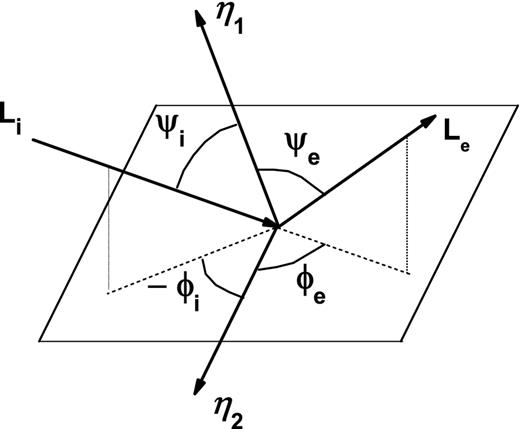
The spacial orientation of the incident and reflected (emergent) radiances, geometrically represented by the light rays Li and Le, for a point in the satellite's surface. ψi and ψe represent the angles between the normal vector to the surface, |$\boldsymbol {\eta _1}$|, respectively, with Li and Le. ϕi and ϕe are obtained by projecting the rays at the plane tangent to the satellite's surface and taking the angles between these projections and the vector |$\boldsymbol {\eta _{2}}$|, parallel to the tangent plane and in the north–south direction (see Appendix A and Fig. A1).
The surface roughness is represented by the variable σ, which is the aperture angle between the facets. It ranges between 0 (perfectly smooth surface) and π/2 (entirely rough surface). Here, we used σ = π/2. In Section 5, we discuss the choice of the reflectance model, and the choice of σ in the fitting of the light curves.
The Oren–Nayar's model requires the determination of the spatial orientation of the incident and reflected radiances stated in equation (2). This requires the computation of the angles shown in Fig. 2. To determine these angles, we used state vectors |$\boldsymbol {V}$|, consisting of the topocentric and heliocentric position and velocity of the satellites and of the Sun (see Fig. 3). They were generated using the DE418, combined with the file NOE–5–2010–GAL.a.bsp through the SPICE information system (Acton 1996). This file, available on the web,3 provided the IMCCE's ephemeris (theory NOE–5–2010) used in this work for the four Galilean satellites (Lainey et al. 2009). Note that the errors in the state vectors from the current ephemeris have a negligible propagation effect in the computed quantities, and can be virtually ignored.
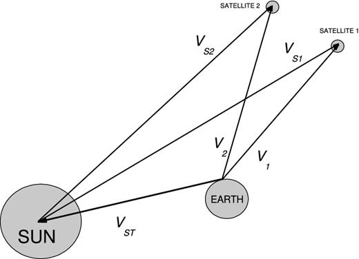
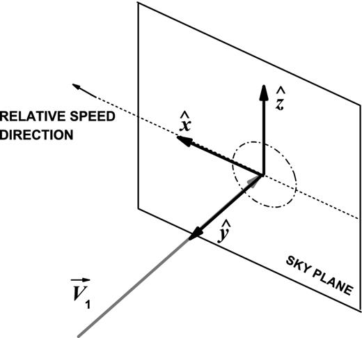
The state vectors of the topocentric position and velocity of the satellites and of the Sun. |$\boldsymbol {V_1}$| is the occulted satellite 1 topocentric position vector. |$\boldsymbol {V_2}$| is the occulting satellite 2 topocentric position vector. |$\boldsymbol {V_{{\rm ST}}}$| is the Sun's topocentric position vector. |$\boldsymbol {V_{{\rm S}1}}$| = (|$\boldsymbol {V_{{\rm ST}}} - \boldsymbol {V_1})$| is the satellite 1 heliocentric position vector. |$\boldsymbol {V_{{\rm S}2}}$| = (|$\boldsymbol {V_{{\rm ST}}} - \boldsymbol {V_2})$| is the satellite 2 heliocentric position vector. For clarity, the velocity components were omitted.
We show in Appendix A how to compute the normal and tangent vectors |$\boldsymbol {\eta _{1}}$| and |$\boldsymbol {\eta _{2}}$|. The topocentric and heliocentric state vectors provide, for each instant, the direction of the incident and scattered light rays (radiances). The orientation of the vectors |$\boldsymbol {\eta _{1}}$| and |$\boldsymbol {\eta _{2}}$| depends of the position of the point in the satellite's surface.
We use these expressions with the Oren–Nayar model to determine the luminous intensity of each point of the disc projected in the sky plane. Note that the effect of the solar phase angle in the projection is naturally accounted for by the reflectance model. Also, the procedure easily identifies when a point in the disc of the occulted satellite lays behind a point in the occulting satellite in front of it. The integration of the (normalized) flux over the two discs gives the total simulated flux of the target satellites for a given instant. We then have the flux of a single point in the simulated light curve. We finally obtain the entire simulated light curve by repeating the procedure for all the instants corresponding to an actual observation.
Importantly, all geometry involving state vectors takes place in a timeless space. Thus, the instants used to generate the state vectors of each satellite and the sun are the instants of each image corrected by the light travel time for each position.
3.3.2 Light-curve simulation for eclipses
The shadow of an eclipse is composed by two regions, the umbra and the penumbra. The flux is zero for points inside the umbra. Inside the penumbra, the flux is attenuated, as compared to a ‘no-eclipse’ situation. Therefore, it is fundamental to rigorously determine the umbra and penumbra regions, for a very precise fitting to the observed light curve of an eclipse.
We geometrically determined the radius of the umbra and penumbra, and semi-analytically derived the gradual decrease of light along the penumbra.
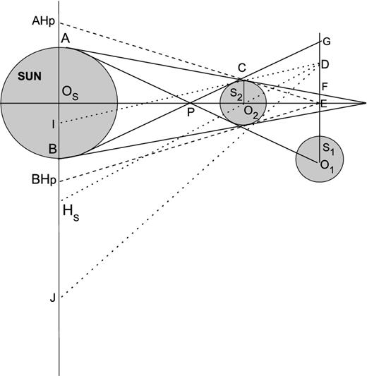
Geometric layout illustrating the radius of the penumbra and umbra, defined at the path GEO1 of the eclipsed satellite. Here, EF = RU (umbra radius), EG = RP (penumbra radius) and OSA = OSB = RS (Sun radius). |$O_{\rm S}O_2 = |\boldsymbol {V_{{\rm S}2}}|$| and |$O_{\rm S}O_1 = |\boldsymbol {V_{{\rm S}1}}|$|, so that the angle between the heliocentric vectors |$\boldsymbol {V_{{\rm S}1}}$| and |$\boldsymbol {V_{{\rm S}2}}$| (see Fig. 3) is |$\arccos \frac{\boldsymbol {V_{{\rm S}1}} \cdot \boldsymbol {V_{{\rm S}2}}}{|\boldsymbol {V_{{\rm S}1}} \cdot \boldsymbol {V_{{\rm S}2}}|}$|. Also, |$O_{\rm S}E=\frac{\boldsymbol {V_{{\rm S}1}} \cdot \boldsymbol {V_{{\rm S}2}}}{|\boldsymbol {V_{{\rm S}2}}|}$|. The solar plane along AOSB contains the Sun, and is normal to the heliocentric vector of the eclipsing satellite. See also the discussion in Appendix B.
We obtained the flux profile of the penumbra by determining the fraction of extinct sun's light along the path of the eclipsed satellite. This was made in two steps.
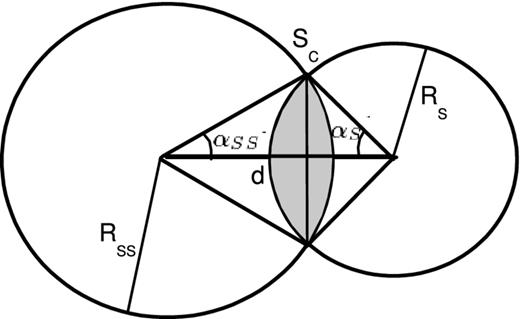
Geometry of a partial occultation. The discs SSS and SS, with radii RSS and RS, respectively, separated by the distance d, overlap each other by the common area Sc.
Here, RS (the Sun radius) and RSS are taken at the solar plane, which is the plane containing the Sun, perpendicular to the heliocentric vector of the eclipsing satellite (see Fig. 4). RSS is the radius of the eclipsing satellite, projected at this plane from the fictitious observer point of view at the penumbra. The calculation of RSS, and the use of RSS, RU and RP in the determination of the actual eclipse shadow cast in the observation plane, including the effect of solar phase, are explained in Appendix B.
The second step consists in taking into account the solar limb darkening, at the uncovered fraction of the solar disc, to calculate the amount of light that is actually received by the satellite. For that, the uncovered solar disc radial profile is numerically represented by rings. Each ring has a light intensity value coherent with the darkening profile proposed by Hestroffer & Magnan (1998). The number of rings was chosen so that the light intensity difference between two consecutive rings was less than 1 per cent, resulting in a smooth limb darkening profile.
Thus, from the obtained penumbra light profile, we determined the incoming and outcoming fluxes Li and Le with the reflectance model, for any point of the eclipsed satellite in the sky plane.
The points of the eclipsed satellite disc projected in the sky, bathed by the umbra, have zero flux. The projected satellite points inside the penumbra have intermediate fluxes, computed by the procedure explained in this section and in Appendix B. Those satellite points outside the penumbra (if any) have fluxes computed by the same procedure described in the previous section. In this way, we derive the luminosity intensity at each point of the satellite disc projected in the sky plane. Integration of all fluxes furnish the (normalized) simulated flux for a given instant. Similarly as before, after considering all the instants, we obtain the entire simulated light curve for the eclipse.
3.4 Ephemeris offsets and ephemeris-based light curves
From state vectors, applying basic plane geometry, we can obtain the impact parameter, the central instant and the relative velocity between two given satellites. Since the state vectors are generated from the ephemeris, these values may be regarded as ephemeris based, and can be compared to the values obtained from actual fits to the observed light curves. A simple transformation translates the differences found into right ascension and declination ‘observed minus ephemeris’ offsets. In fact, this information is stored in the fitting procedures.
The fitting software constructs a light curve from values for the impact parameter, relative velocity and central instant. This allows for a visual inspection during the fitting procedure, from starting values to the final results themselves. The ephemeris-based computed values are also used to generate ephemeris-based light curves, that can be compared to the observed and fitted ones.
All this allows for both a qualitative and quantitative comparison between observation and ephemeris.
4 RESULTS
We fitted the light curves of 25 events and obtained the values and error estimates for the impact parameter, the relative velocity and the central instant, following the procedures described in Section 3. We also calculated these parameters from the ephemeris, as explained in Section 3.4. This allowed us to compare the expected results from the ephemeris with the observed ones. Figs 6 and 7 illustrate two examples of adjustment of light curves from an eclipse and from an occultation. The ephemeris-based light curves are also displayed. In Appendix C, we illustrate all the events. Figs C1 to C3 (occultations) and C4 to C6 (eclipses) sample the events according to the quality of the observations and adjustments, i.e. ‘excellent’, ‘good’ and ‘regular’.
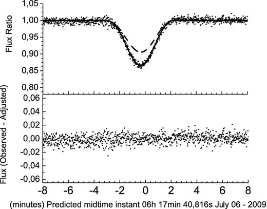
Light-curve fit for the eclipse of Europa by Io in 2009 July 06. Top: the observed light curve (dots), the fitted light curve (solid line) and the computed ephemeris-based light curve (dashed line). Bottom: the difference between the observed and the fitted curves (O − C), showing the quality of the adjustment. Time is in UTC.
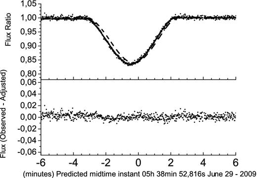
Light-curve fit for an occultation of Europa by Io in 2009 June 29. Top: the observed light curve (dots), the fitted light curve (solid line) and the computed ephemeris-based light curve (dashed line). Bottom: the difference between the observed and the fitted curves (O − C), showing the quality of the adjustment. Time is in UTC.
We show in Table 2 (for occultations) and in Table 3 (for eclipses) the parameters and respective errors obtained from the light-curve fits of all the events. For the impact parameter and the velocity, values are listed in kilometres and kilometres per second, and in milliarcseconds and milliarcseconds per second, respectively. For the central instant, in UTC (Universal Time Coordinated), the label of each event indicates the day and month. We list the instant in hours, minutes and seconds, and the error in seconds and in kilometres (by the use of the relative velocity in kilometres per second). We also list in Tables 2 and 3 the photometric error, based on the dispersion of light-curve points outside the events, and the mean error in flux ratio, computed from the light-curve fits. The ratio of albedos (and errors) used for the light-curve reduction of the occultations (see Section 3.2) are also given in Table 2.
Results for the occultations.
| Event | Impact | ΔIP | Relative | ΔRV | Central | ΔMI | Δαcos δ | Δδ | Photo. | σfit | Ratio of |
|---|---|---|---|---|---|---|---|---|---|---|---|
| parameter | velocity | instant | error | Albedos | |||||||
| (km) | (km) | (km s−1) | (km s−1) | (h m s) | (s) | (km) | (km) | ×10−2 | ×10−2 | ||
| (mas) | (mas) | (mas s−1) | (mas s−1) | σMI(km) | (km) | (mas) | (mas) | ||||
| 2704GoI | 381.2 (33.2) | −93.5 | 23.77(0.08) | −0.025 | 06 42 43.24(0.22) | −6.89 | 146.7 | −118.5 | 1.09 | 1.11 | 1.67(0.08) |
| 99.8 (8.7) | −24.5 | 6.22(0.019) | −0.01 | 5.22 | −164.0 | 38.4 | −31.8 | ||||
| 0905EoI | 2060.7 (10.4) | 46.97 | 28.86(0.37) | 1.48 | 07 21 48.34(0.56) | −8.03 | 37.6 | −220.9 | 4.46 | 1.5 | 0.88(0.01) |
| 554.5 (2.7) | 12.7 | 7.81(0.10) | 0.4 | 15.7 | −230.0 | 10.2 | −59.9 | ||||
| 2105IoE | 229.2 (29.1) | 183.83 | 22.65(0.10) | 0.10 | 05 29 35.71(0.29) | −10.6 | −82.4 | −290.5 | 2.29 | 1.51 | 1.04(0.14) |
| 64.5 (8.2) | 51.8 | 6.38(0.029) | 0.03 | 6.6 | −240.6 | −23.2 | −81.8 | ||||
| 2805IoE | 602.2 (6.1) | −15.28 | 21.95(0.05) | 0.31 | 07 44 08.73(0.16) | −10.9 | 101.7 | −213.7 | 1.12 | 0.8 | 1.01(0.01) |
| 173.5 (1.8) | −4.41 | 6.32(0.015) | 0.09 | 3.5 | −239.6 | 29.3 | −61.6 | ||||
| 2206IoE | 1805.6 (8.9) | 13.3 | 19.27(0.18) | 1.00 | 03 27 46.91(0.60) | −8.05 | 42.10 | −141.7 | 0.11 | 1.3 | 0.98(0.007) |
| 562.9 (2.8) | 4.1 | 6.01(0.054) | 0.31 | 11.6 | −155.3 | 13.1 | −44.1 | ||||
| 2906IoE | 1867.6 (2.9) | −27.5 | 17.44(0.053) | 0.19 | 05 38 20.71(0.22) | −10.2 | 90.2 | −153.1 | 0.07 | 0.4 | 0.97(0.005) |
| 594.2 (0.9) | −8.8 | 5.54(0.017) | 0.06 | 3.9 | −177.4 | 28.7 | −48.7 | ||||
| 0607IoE | 1861.2 (4.0) | −38.5 | 15.55(0.064) | −0.66 | 07 48 27.18(0.34) | −6.32 | 73.3 | −81.3 | 0.05 | 0.6 | 1.00(0.006) |
| 603.3 (1.3) | −12.4 | 5.04(0.021) | −0.21 | 5.3 | −98.3 | 23.7 | −26.3 | ||||
| 0708IoE | 818.7 (4.4) | −87.1 | 10.45(0.022) | −0.52 | 05 37 45.58(0.31) | −7.25 | 109.5 | −44.3 | 0.56 | 0.8 | 0.93(0.011) |
| 279.4 (1.5) | −29.7 | 3.56(0.007) | −0.2 | 3.2 | −75.8 | 37.3 | −15.9 | ||||
| 1208GoE | 3132.4 (2.5) | −27.8 | 7.94(0.031) | 0.12 | 2 11 2.54(0.63) | 14.3 | −15.0 | 114.4 | 0.46 | 0.4 | 1.68(0.000) |
| 1066 (0.8) | −9.5 | 2.70(0.011) | 0.04 | 5.0 | 113.6 | −5.1 | 39.1 | ||||
| 2208IoE | 1938.7 (2.0) | −19.7 | 5.45(0.012) | 0.18 | 04 07 55.99(0.52) | 6.85 | 4.75 | 40.8 | 0.05 | 0.5 | 0.93(0.011) |
| 661.1 (0.7) | −6.7 | 1.84(0.004) | 0.06 | 2.8 | 37.4 | 1.6 | 13.9 | ||||
| 1609IoE | 1685.2 (5.9) | −68.6 | 11.04(0.059) | −0.19 | 00 46 13.50(0.64) | 5.38 | 42.9 | 80.8 | 0.01 | 1.1 | 1.01(0.008) |
| 556.2 (1.9) | −22.6 | 3.64(0.019) | −0.06 | 7.0 | 59.4 | 14.2 | 26.6 | ||||
| 2410GoE | 2259.9 (4.6) | −58.2 | 13.72(0.049) | −0.20 | 00 35 47.84(0.42) | 19.2 | −34.4 | 271.4 | 13.5 | 0.8 | 1.68(0.087) |
| 670.5 (1.3) | −17.2 | 4.07(0.015) | −0.01 | 5.8 | 263.3 | −10.2 | 80.5 | ||||
| 2510IoE | 1892.0 (17.1) | −55.7 | 19.47(0.358) | 1.48 | 01 21 43.70(1.20) | 14.1 | −34.8 | 258.0 | 0.01 | 1.4 | 1.01(0.008) |
| 558.9 (4.7) | −16.5 | 5.70(0.105) | 0.44 | 23.4 | 275.3 | −10.3 | 76.3 |
Note. The results are arranged in two rows for each event. The values in parentheses are their respective errors. The impact parameter and the relative velocity are listed in the first line, respectively, in kilometres and kilometres per second, and in the second line in milliarcseconds and milliarcseconds per second. For the central instant, in UTC, the label of each event indicates the day and month, and the first line gives the instant in hours, minutes and seconds. The second line (σMI) lists the mid-time instant error in kilometres, by the use of the relative velocity in kilometres per second. ΔIP, ΔRV and ΔMI are the respective differences between the fitted parameters and the ephemeris-based values in the sense ‘observation − ephemeris’. In columns 8 and 9, we also list the (Δαcos δ, Δδ) orbital offsets in the sense ‘observation − ephemeris’. The photometric errors are based in the dispersion of the light-curve points outside the events. The σfit values are the mean error in the flux ratio, computed from the light-curve fits. The listed ratio of albedos were computed following the procedures described in Section 3.2. For 1208GoE, the ratio of albedos was not directly determined from observations before and after the event. Instead, we computed it by multiplying the values of the ratio of albedos of the event 2704GoI, and the average value for Io/Europa ratio of albedos obtained from the events 0708IoE, 2208IoE and 1609IoE. These events were observed close to the 1208GoE occultation.
Results for the eclipses.
| Event | Impact | ΔIP | Relative | ΔRV | Central | ΔMI | Δαcos δ | Δδ | Photo. | σfit |
|---|---|---|---|---|---|---|---|---|---|---|
| parameter | velocity | instant | error | |||||||
| (km) | (km) | (km s−1) | (km s−1) | (h m s) | (s) | (km) | (km) | ×10−2 | ×10−2 | |
| (mas) | (mas) | (mas s−1) | (mas s−1) | σMI(km) | (km) | (mas) | (mas) | |||
| 1006GeC | 1151.5 (5.5) | 85.7 | 14.62(0.02) | 0.19 | 07 29 40.25(0.21) | 14.9 | −160.9 | 166.39 | 0.57 | 1.0 |
| 345.6 (1.7) | 25.7 | 4.39(0.005) | 0.06 | 3.1 | 217.9 | −48.3 | 50.0 | |||
| 1606GeI | 3422.8 (1.8) | 108.2 | 5.50(0.016) | 0.08 | 08 45 4.17(0.73) | −41.6 | 14.83 | 249.7 | 0.79 | 0.9 |
| 1050 (0.5) | 33.2 | 1.69(0.005) | 0.02 | 3.0 | −228.8 | 4.5 | 76.6 | |||
| 1906CeE | 1783.0 (2.6) | −23.6 | 19.09(0.026) | −0.55 | 05 11 37.02(0.14) | 5.46 | −16.65 | 102.74 | 1.53 | 0.7 |
| 551.0 (0.8) | −7.3 | 5.90(0.008) | −0.17 | 2.7 | 104.4 | −5.14 | 31.7 | |||
| 1906CeI | 3393.2 (3.0) | 8.3 | 18.94(0.072) | −0.39 | 08 32 50.77(0.34) | 6.50 | −55.3 | 113.3 | 0.95 | 0.6 |
| 1049 (0.9) | 2.5 | 5.85(0.022) | −0.12 | 6.4 | 123.2 | −17.1 | 39.9 | |||
| 2006CeI | 1926.4 (1.6) | −1.5 | 4.89(0.005) | 0.36 | 05 09 49.65(0.38) | −20.4 | −36.9 | 84.7 | 2.06 | 0.9 |
| 597.9 (0.5) | −0.5 | 1.52(0.002) | 0.11 | 1.9 | −99.9 | −11.4 | 26.3 | |||
| 2006CeI | 1517.4 (3.9) | −15.5 | 5.06(0.007) | 0.008 | 09 37 20.90(0.51) | 22.0 | −27.4 | 109.2 | 4.69 | 1.4 |
| 471.1 (1.1) | −4.8 | 1.57(0.002) | 0.002 | 2.6 | 111.6 | −8.5 | 33.8 | |||
| 0407IeG | 1486.9 (6.3) | −15.42 | 26.70(0.068) | 0.07 | 06 25 14.90(0.19) | 1.97 | −5.49 | 54.4 | 0.08 | 0.7 |
| 479.1 (2.0) | −4.97 | 8.59(0.021) | 0.02 | 5.1 | 52.6 | −1.7 | 17.5 | |||
| 0607IeE | 2487.8 (3.4) | −167.8 | 19.01(0.122) | 1.33 | 06 17 16.94(0.39) | 0.16 | 154.8 | 64.9 | 0.56 | 0.6 |
| 806.3 (1.1) | −54.3 | 6.16(0.040) | 0.43 | 7.4 | 3.00 | 50.2 | 21.0 | |||
| 0807GeI | 777.8 (4.1) | −58.4 | 22.23(0.018) | 0.28 | 08 31 15.12(0.07) | 9.2 | −21.9 | 208.7 | 0.15 | 0.7 |
| 253.5 (1.4) | −19.0 | 7.25(0.006) | 0.09 | 1.6 | 204.2 | −7.13 | 68.0 | |||
| 1307IeE | 2312.8 (3.9) | 21.9 | 17.04(0.104) | 0.54 | 08 38 47.04(0.43) | 1.02 | −26.6 | 7.63 | 1.19 | 1.2 |
| 762.1 (1.3) | 7.2 | 5.62(0.003) | 0.01 | 7.3 | 17.5 | −8.7 | 2.51 | |||
| 0708IeE | 1656.7 (5.2) | 178.9 | 11.21(0.052) | −0.21 | 05 14 55.88(0.58) | 3.16 | −180.1 | −29.4 | 0.02 | 2.3 |
| 568.6 (1.7) | 61.0 | 3.77(0.017) | −0.07 | 6.5 | 35.5 | −61.5 | −10.0 | |||
| 1609IeE | 576.2 (14.0) | −67.6 | 13.34(0.065) | 0.36 | 02 15 9.96(0.54) | −0.66 | 66.3 | 15.7 | 0.60 | 4.4 |
| 190.1 (4.5) | −22.3 | 4.40(0.022) | 0.11 | 7.2 | −8.84 | 21.9 | 5.2 |
Note. Read definitions in Table 2. We do not list the ratio of albedos, as this is not used in the reductions of eclipses.
We compared the results with the ephemeris published by the IMCCE, currently considered the most accurate representative for the Jovian system. We list in Tables 2 and 3 the differences between the fitted and the ephemeris-based parameter values. We also list the (Δαcos δ, Δδ) orbital offsets in the sense ‘observation − ephemeris’.
5 THE REFLECTANCE LAW
The choice of the reflectance law has great influence in the light-curve fit of the mutual events. This is because the satellite's photocentre is significantly offset relative to its geometric centre, if the solar phase angle is not negligible. Therefore, the choice of the reflectance model affects the relationship between the impact parameter and the light-curve's depth. Another possible side effect is the bad determination of the central instant. Thus, the choice of a simple or incorrect reflectance model may lead to a less precise, possibly inaccurate determination of the parameters, depending on the photometric quality of the light curve. As a consequence, the mean error of the fits in flux ratio may increase. We used the computed mean errors of some selected light curves as a guide to measure the adequateness of some tested reflectance models. The final choice was made according to the quality of the fit obtained from these light curves.
Knowing that the Poisson noise is proportional to the square root of the intensity of the object's light flux, a decrease in brightness, as observed close to the central instant of some events (mostly central eclipses), causes a decrease in the noise, and hence, in the dispersion of the points near the bottom of the light curve. A narrowing is observed in the light curve near the central instant for such events. Fig. 8 displays an example.
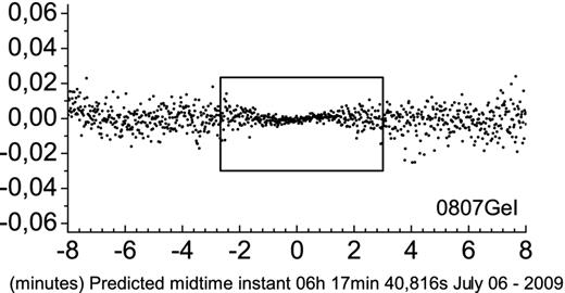
Bottom part of the light curve of the event 0807GeI (from Fig. C4) showing the narrowing observed due to a noise reduction, as a consequence of the flux drop from the target, due to the passage of the shadow (central eclipse).
In the Poisson noise regime (as is the case of our observations), we should expect that the photometric error is minimum at the bottom of the light curve, thus making this part of the light curves suitable for the analysis of the reflectance model. If the reflectance model does not provide a good fit, the bottom part of the theoretical light curve should be slightly offset from the observed one, due to the bad determination of the impact parameter and, possibly, also of the central instant. This effect is shown in Fig. 9. Therefore, besides the inspection of the mean error of the flux ratio, computed from the light-curve fits, this behaviour is another factor that helps in the choice of the reflectance model.
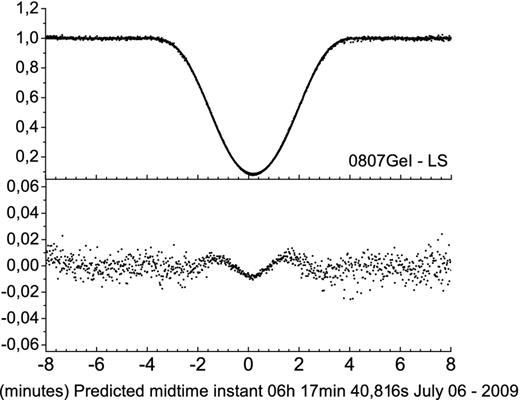
Light-curve fit for the eclipse of Io by Ganymedes in 2009 July 08 using the Lommel-Seelinger reflectance model (0807GeI - LS). Top: the observed light curve (dots) and the fitted light curve (solid line). Bottom: the difference between the observed and the fitted curves (O − C), showing the failure to determine the central instant which causes a horizontal offset between the fitted and the observed light curve. Time is in UTC.
The most basic and commonly used light scattering model is the simple Lambert's scattering law. It assumes an infinite-sized source of light, and a reflecting surface that scatters the incident light equally in all directions. Therefore, the satellite's surface luminosity can be represented by a homogeneous grey disc. In this case, one way to account for the solar phase angle is to describe the format of the apparent disc as a combination of a semicircle with a semi-ellipse. However, the high photometric quality of the observed events makes this model too simplistic and, therefore, inappropriate to provide a high-quality fit to our light curves.
Here, f(α) = 1 + Bα + Cα2 is the phase function of the surface, where α is the phase angle, ψi and ψe are the same as in Fig. 2, A is a function of α and the parameters B and C depend of the satellites surface features. Unfortunately, in the literature, there was no information about these parameters for the Galilean satellites (except for Europa), for the wavelength range covered by this study. Therefore, this model could not be further tested.
Hapke's scattering law (Hapke 1981, 1984) is a sophisticated model that has been used in some works. Unfortunately, we could not apply it, due to the severe lack of information on many of the parameters of that law, for the wavelength band of our observations – as was the case with the generalized version of Lommel-Seelinger's law. We notice, however, that Emelyanov (2009) (see Section 4, table 2 in that article), reports that both the Hapke's and Lommel-Seelinger's laws have a similar performance.
We finally found the solution as a generalization of Lambert's law (Oren & Nayar 1994), that takes into account not only the direction of the radiances, like the other models, but also the surface roughness. The roughness is represented by a factor of σ, which ranges between 0 and π/2, with π/2 equivalent to the surface roughness of a full Moon. The Oren–Nayar's model proved to be efficient in describing the profile of spherical surfaces illuminated by a finite source, and then we decided to test it.
The first test was to verify the model's capacity to solve the problem pointed out in Fig. 9. The results were highly satisfactory, as shown in Fig. 10.
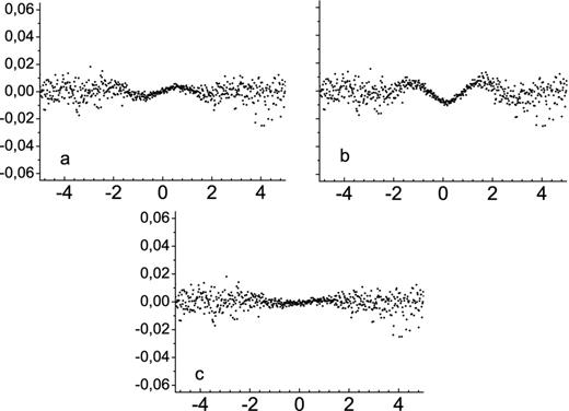
Small zoom near the mid-time instant in the curve (O − C) of the event 0807GeI comparing the three reflection models tested. Top: (a) Lambert's simple law and (b) Lommel-Seelinger's law in the right. Bottom: (c) Oren–Nayar's model. Time is in UTC.
We then verified if there were a strong dependence of the model with the parameter σ describing the surface roughness. If we found a high dependence, we should consider fitting this parameter too. However, changing the value of σ did not produce significant changes in the parameters of the light curve. Also, no significant changes occurred in the mean error of the flux ratio (σfit). This indicates that the Oren–Nayar's model is a very robust reflectance model, even for high-precision photometric light curves. One advantage of this model is that no ad hoc albedo-wavelength-related parameters need to be set for the satellites, as is the case of other reflectance laws used in the literature. Thus, the Oren–Nayar's model is a very interesting alternative, that can be used in the light-curve fit of mutual events of any giant planet, without a priori photometric knowledge in the satellites. Taking into account the recommendations in Oren & Nayar (1994), we used σ = π/2 in our fits. The simplified version of the model was used. Due to our photometric precision, it furnishes the same results as the complete model, in much less computing time.
6 CONCLUSIONS
We presented the results obtained from the observation, reduction and analysis of 25 mutual events registered during the Brazilian campaign for the observation of mutual phenomena between the Galilean satellites.
The narrow-band filter at 890 nm, combined with the differential photometry and the refined procedures in the fitting of the light curves developed in this work, resulted in average precisions of 80.1 m s−1 (0.023 mas s−1) and 7.46 km (2.19 mas) for the relative velocity and impact parameter (relative positions), respectively, and 0.42 s (6.13 km) for the central instant.
The extensive use of numerical procedures with analytical and semi-analytical models, allowed for a complete, rigorous implementation of the complex geometry involved in describing the flux drop in occultations and eclipses. The modelling of the solar limb darkening and the implementation of the computation of the gradual decrease of light over the shadow in an eclipse are examples. This also allowed for the analysis of different reflective laws and models in a fast and direct way. Through this analysis, we were able to highlight and study the relation between the impact parameter and the reflective model. From this study, we could finally adopt a generalized reflectance model – the Oren–Nayar's model, used for the first time in a work on occultations and eclipses in mutual events. This model is well suited for fitting high-precision light curves, and does not depend on wavelength and other a priori photometric knowledge of the satellites, contrary to some reflectance models currently in use. We emphasize that our developed light-curve fitting procedures are ephemeris-independent, thus allowing for an unbiased comparison with the current orbit implementations available for the Galilean satellites.
The tools and techniques developed and used in this work, allowed for a comprehensive analysis of the many factors inherent to the nature of these events. They will be of great utility in future campaigns, not restricted to the Jupiter system. The use of more powerful detectors will possibly make it easier to study new refinements in the analysis.
We thank Dr W. Beisker, president of the IOTA-ES (International Occultation Timing Association - European Section) for kindly providing the methane filter used in our observations. We also thank Dr N. Emelyanov, of the Sternberg Astronomical Institute – Moscow, for the fruitful discussions about the light-curve adjustments. The ephemerides and data on the NOE–5–2010 file are issued from the activity of the Bureaux des Longitudes in Celestial Mechanics and Astrometry. MA, JIBC and RVM acknowledge CNPq/Brazil grants 482080/2009-4, 306028/2005-0, 478318/2007-3, 151392/2005-6 and 304124/2007-9. MA and JIBC thank FAPERJ/Brazil for grants E-26/170.686/2004 and E-26/110.177/2009. ADO and FBR thanks the financial support by the CAPES/Brazil.
Based on observations made at the Laboratório Nacional de Astrofísica (LNA), Itajubá-MG, Brazil.
REFERENCES
APPENDIX A: COMPUTING VECTORS η1 AND η2 FOR SIMULATING LIGHT CURVES
In the occultation case, and outside the umbra and penumbra in the eclipse case, we sweep the two-dimensional sky plane, integrating the reflected (emergent) radiance Le, in order to determine the flux value at each (x, z) point in that plane. In this way, we obtain the light intensity profile of the satellite discs projected in the sky plane – a necessary step in the simulation of the light curves. We obtain Le by equation (2), following the Oren–Nayar's reflectance model. The angles in equation (2) are computed from equations (6) to 9, which depend on the normal and tangent vectors |$\boldsymbol {\eta _{1}}$| and |$\boldsymbol {\eta _{2}}$|. Here, we show how we obtained |$\boldsymbol {\eta _{1}}$| and |$\boldsymbol {\eta _{2}}$| using spherical geometry.
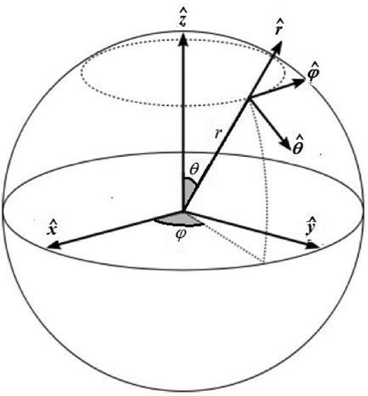
The spherical coordinate system with origin at the centre of the satellite. The vectors |$\boldsymbol {\eta _{1}}$| and |$\boldsymbol {\eta _{2}}$|, from Fig. 2, point in the direction of |$\hat{r}$| and |$\hat{\theta }$|, respectively.
The xz plane of the associated Cartesian coordinate system of Fig. A1 coincides with the sky plane. |$\boldsymbol {\hat{x}}$|, |$\boldsymbol {\hat{y}}$| and |$\boldsymbol {\hat{z}}$| are the unitary vectors in x, y and z directions, respectively.
APPENDIX B: COMPUTING THE FRACTION OF SUNLIGHT IN ECLIPSES
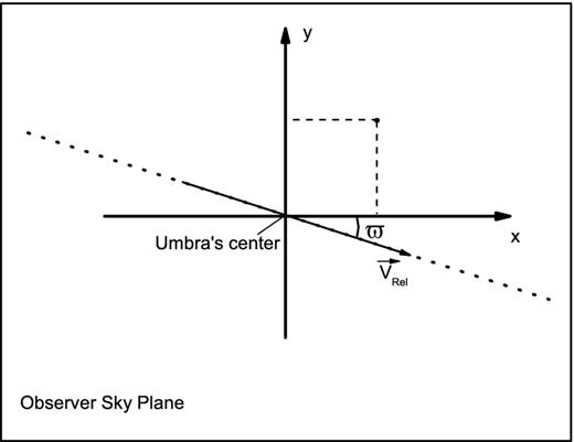
Coordinate system at the observation plane where the y-axis is normal to the plane containing the solar phase angle.
The (x, y) are the coordinates of a point in the penumbra with respect to the umbra centre at the observation plane. Using equations (B1) to B4, we sweep the (x, y) coordinates of this plane, considering the regions delimited by the computed umbra and penumbra radii, RU and RP. Taking the solar limb darkening into account, we then determine the effective light Li received by the eclipsed satellite, for each point in the sky. We then use the reflectance model to obtain the reflected light Le.
Comparing the shadow cones represented by the triangles AHpEBHp and IDJ in Fig. 4, we note that, for a fictitious observer located inside the umbra and penumbra (point D), the radius RSS of the disc projected in the solar plane undergoes a small variation, as we move along the segment EG. The amount of this variation depends on the distance between the satellites and the Sun, and on their radii. For all the events of this work, the maximum variation of RSS remained below 0.15 per cent, after considering the two extreme cases: observer located at the centre of the umbra (point E), and located at the edge of the penumbra (point G). This negligible effect was thus ignored, and we adopted the simple calculation of RSS using the triangle AHpEBHp alone (see Fig. 4).
APPENDIX C: LIGHT CURVES OF THE EVENTS
Here, we present the reduced light curves of the events treated in this work. The figures are divided by the quality of the light curves and respective events’ codes are indicated in each figure.
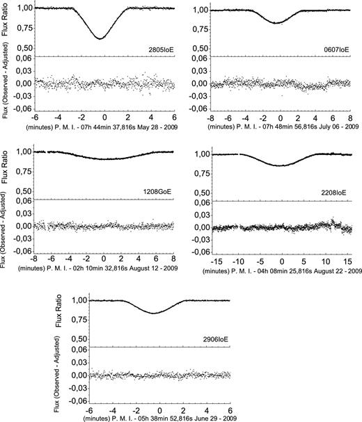
Five occultations’ light curves classified as excellent. For each curve, Top: the Observed light curve (dots) and the fitted curve (solid line). Bottom: the difference between the observed and fitted curves (O − C), showing the quality of the adjustment. The x-label of each curve indicates the time unit (in UTC), where P.M.I stands for predicted central instant.
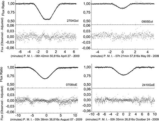
Four occultations’ light curves classified as good, with the same layout of Fig. C1.
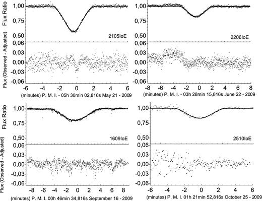
Four occultations’ light curves classified as regular, with the same layout of Fig. C1.
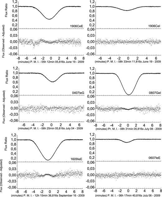
Six eclipses’ light curves classified as excellent. For each curve, Top: the Observed light curve (dots) and the fitted curve (solid line). Bottom: the difference between the observed and fitted curves (O − C), showing the quality of the adjustment. The x-label of each curve indicates the time unit (in UTC), where P.M.I stands for predicted central instant.
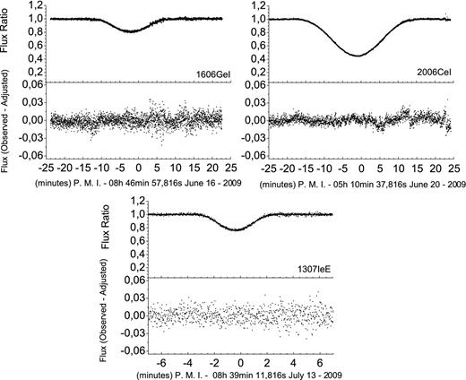
Three eclipses’ light curves classified as good, with the same layout of Fig. C4.
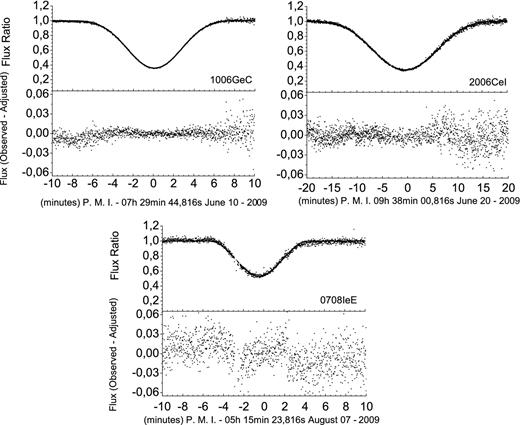
Three eclipses’ light curves classified as regular, with the same layout of Fig. C4.
Author notes
E-mail: [email protected]
