


Abstract
Asteroseismic data can be used to determine stellar surface gravities with precisions of <0.05 dex by using the global seismic quantities 〈Δν〉 and νmax along with standard atmospheric data such as Teff and metallicity. Surface gravity is also one of the four stellar properties to be derived by automatic analyses for one billion stars from Gaia data (workpackage gsp_phot). In this paper, we explore seismic data from main-sequence F, G, K stars (solar-like stars) observed by the Kepler spacecraft as a potential calibration source for the methods that Gaia will use for object characterization (log g). We calculate log g for some bright nearby stars for which radii and masses are known (e.g. from interferometry or binaries), and using their global seismic quantities in a grid-based method, we determine an asteroseismic log g to within 0.01 dex of the direct calculation, thus validating the accuracy of our method. We also find that errors in adopted atmospheric parameters (mainly [Fe/H]) can, however, cause systematic errors of the order of 0.02 dex. We then apply our method to a list of 40 stars to deliver precise values of surface gravity, i.e. uncertainties of the order of 0.02 dex, and we find agreement with recent literature values. Finally, we explore the typical precision that we expect in a sample of more than 400 Kepler stars which have their global seismic quantities measured. We find a mean uncertainty (precision) of the order of better than 0.02 dex in log g over the full explored range 3.8 < log g < 4.6, with the mean value varying only with stellar magnitude (0.01–0.02 dex). We study sources of systematic errors in log g and find possible biases of the order of 0.04 dex, independent of log g and magnitude, which accounts for errors in the Teff and [Fe/H] measurements, as well as from using a different grid-based method. We conclude that Kepler stars provide a wealth of reliable information that can help to calibrate methods that Gaia will use, in particular, for source characterization with gsp_phot, where excellent precision (small uncertainties) and accuracy in log g is obtained from seismic data.
1 INTRODUCTION
Large-scale surveys provide a necessary homogenous set of data for addressing key scientific questions. Their science-driven objectives naturally determine the type of observations that will be collected. However, to fully exploit the survey, complementary data, either of the same type but measured with a different instrument or of a different observable, need to be obtained. Combining data from several large-scale surveys can only result in the best exploitation of both types of data.
The ESA Gaia mission1 is due for launch in 2013 Autumn. Its primary objective is to perform a six-dimensional mapping of the Galaxy (three positional and three velocity data)2 by observing over one billion stars down to a magnitude of V = 20. The mission will yield distances to these stars, and for about 20/100 million stars distances with precisions of less than 1 per cent/10 per cent will be obtained.
Gaia will obtain its astrometry by using broad-band G photometry.3 The spacecraft is also equipped with a spectrophotometer comprising both a blue and a red prism BP/RP, delivering colour information. A spectrometer will be used to determine the radial velocities of objects as far as G = 17 (typical precisions range from 1 to 20 km s−1), and for the brighter stars (G < 11) high-resolution spectra (R ∼ 11 500) will be available.
One of the main workpackages devoted to source characterization is gsp_phot whose objectives are to obtain stellar properties for one billion single stars by using the G-band photometry, the parallax π and the spectrophotometric information BP/RP (Bailer-Jones 2010). The stellar properties that will be derived are effective temperature Teff, surface gravity log g, and metallicity [Fe/H], and also extinction AG in the astrometric G band to each of the stars. Liu et al. (2012) discuss several different methods that were developed to determine these parameters using Gaia data and we refer to this paper and references within for details. In brief, they discuss the reliability of determining the four parameters by using simulations, and in particular, they conclude that they expect typical precisions in log g of the order of 0.1–0.2 dex for main-sequence late-type stars, with mean absolute residuals (true value minus inferred value from simulations) no less than 0.1 dex for stars of all magnitudes, see figs 14 and 15 of Liu et al. (2012). We note that the stellar properties derived by gsp_phot will be used as initial input parameters for the workpackage devoted to detailed spectroscopic analysis of the brighter targets gsp_spec (Recio-Blanco, Bijaoui & de Laverny 2006; Bijaoui et al. 2010; Kordopatis et al. 2011; Worley et al. 2012) using the radial velocity spectrometer data (Katz 2005). Spectroscopic determinations of log g, Teff and [Fe/H] in general can have large correlation errors, and if log g is well constrained, Teff, [Fe/H] and chemical abundances can be derived more precisely.
The different algorithms for gsp_phot discussed by Liu et al. (2012) used to determine the stellar properties in an automatic way have naturally been tested on synthetic data. However, to ensure the validity of the stellar properties, a set of 40 bright benchmark stars have been compiled and work is still currently underway to derive stellar properties for all of these in the most precise, homogenous manner (e.g. Heiter et al., in preparation). Unfortunately, these benchmark stars will be too bright for Gaia, and so a list of about 500 primary reference stars has also been compiled. The idea is to use precise ground-based data and the most up-to-date models (known from working with the benchmark stars) to determine their stellar properties as accurately (correct) and precisely (small uncertainties) as possible. These primary reference stars will be observed by Gaia and thus will serve as a set of calibration stars. A third list of secondary reference stars has also been compiled. These consist of about 5000 fainter targets.
In the last decade or so, much progress in the field of asteroseismology has been made, especially for stars exhibiting Sun-like oscillations. These stars have deep outer convective envelopes where stochastic turbulence gives rise to a broad spectrum of resonant oscillation modes (e.g. Ulrich 1970; Leibacher & Stein 1971; Brown & Gilliland 1994; Salabert et al. 2002; Bouchy & Carrier 2002). The power spectrum of such stars can be characterized by some global seismic quantities: 〈Δν〉, νmax and 〈δν〉. The quantity 〈Δν〉 is the mean value of the large frequency separations Δνl, n = νl, n − νl, n−1 where νl, n is a resonant oscillation frequency with degree l and radial order n, νmax is the frequency corresponding to the maximum of the bell-shaped frequency spectrum, and 〈δν〉 is the mean value of the small frequency separations δνl, n = νl, n − νl + 2, n−1. Fig. 1 shows the power (frequency) spectrum of a solar-like star, observed by the Kepler spacecraft, depicting these quantities.
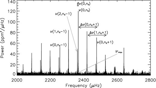
High S/N power/frequency spectrum of a Kepler solar-like star KIC 6603624. Some individual frequencies ν are denoted with their degree l and radial order n in parenthesis (Appourchaux et al. 2012). The reference radial order n0 usually corresponds to orders similar to 20 for these stars. We also show the individual large and small frequency separations, Δν(l, n) and δν(l, n), respectively, for three cases, and the approximate frequency corresponding to the maximum power in the spectrum, νmax. For much lower S/N spectra, the mean value 〈Δν〉 of the large frequency separations and νmax can usually be determined even if individual frequencies ν cannot be resolved.
Even when individual frequencies cannot be determined from the frequency spectra both 〈Δν〉 and νmax can still be extracted quite robustly. Many methods have been developed to do this using Kepler-like data (Bonanno et al. 2008; Huber et al. 2009; Mosser & Appourchaux 2009; Campante et al. 2010; Hekker et al. 2010; Karoff et al. 2010; Mathur et al. 2010b) and these have been compared in Verner et al. (2011) (see references therein). The global seismic quantities have been shown to scale with stellar parameters such as mass, radius and Teff e.g. (Brown & Gilliland 1994; Bedding & Kjeldsen 2003; Stello et al. 2008; Bedding 2011; Huber et al. 2011; Miglio et al. 2012; Silva Aguirre et al. 2012). By comparing the theoretical seismic quantities with the observed ones over a large grid of stellar models, very precise determinations of log g (<0.05 dex) and mean density (<2 per cent) can be obtained for main-sequence F, G, K stars (Bruntt et al. 2010; Metcalfe et al. 2010; Gai et al. 2011; Creevey et al. 2012a; Mathur et al. 2012).
Of particular interest for Gaia is the Kepler4 field of view, ∼100 square degrees, centred on galactic coordinates 76|${^{\circ}_{.}}$|32, +13|${^{\circ}_{.}}$|. Kepler is a NASA mission dedicated to characterizing planet-habitability (Borucki et al. 2010). It obtains photometric data of approximately 150 000 stars with a typical cadence of 30 min. However, a subset of stars (less than 1000 every month) acquires high-cadence data with a point every 1 min. This is sufficient to detect and characterize Sun-like oscillations in many stars. Verner et al. (2011) and Chaplin et al. (2011) recently showed the detections of the global seismic quantities for a sample of 600 F, G, K main sequence and subgiant (V/IV) stars with typical magnitudes 7 < V < 12, while both CoRoT and Kepler have both shown their capabilities of detecting these same seismic quantities in thousands of red giants, e.g. (Hekker et al. 2009; Bedding et al. 2010; Kallinger et al. 2010b; Baudin et al. 2011; Mosser et al. 2012; Stello et al. 2013).
With the detection of the global seismic quantities in hundreds of main-sequence stars (and thousands of giants), the Kepler field is very promising for helping to calibrate Gaiagsp_phot methods. In particular, the global seismic quantities deliver one of the four properties to be extracted by automatic analysis, namely log g. Gai et al. (2011) studied the distribution of errors for a sample of simulated stars using seismic data and a grid-based method based on stellar evolution models. They concluded that log g derived from seismic properties (‘seismic log g’) is almost fully independent of the input physics in the stellar evolution models that are used. More recently, Morel & Miglio (2012) compared classical determinations of log g to those derived alone from a scaling relation (see equation 2), and concluded that the mean differences between the various methods used is ∼0.05 dex, thus supporting the validity of a seismic determination of log g. While some studies have focused on comparing seismic radii or masses with alternative determinations, for example, Bruntt et al. (2010), no study has been done focusing on both the accuracy and precision of a seismic log g using one or more grid-based methods for stars with accurately measured radii and masses. The accuracy and precision in log g for these bright stars has also not been tested while considering precisions in data such as those obtained by Kepler. Such a study could validate the use of seismic data as a calibration source for Gaia. For the rest of this work the term precision refers exclusively to the derived uncertainty in log g, while accuracy refers to how true the value is.
With these issues in mind, the objectives of this paper are to (i) test the accuracy and precision of a seismic log g from a grid-based method using bright nearby targets for which radii and masses have been measured (Section 3), (ii) determine log g for an extended list of stars whose global seismic properties and atmospheric parameters are available in the literature using the validated method (Section 4) and (iii) study the distribution of log g and their uncertainties of over 400 F, G, K V/IV Kepler stars derived by a grid-based method while concluding on realistic uncertainties (precisions) and possible sources of systematic errors for this potential sample of Gaia calibration stars (Section 5). In this work, our analysis is restricted to stars with log g > 3.75 primarily due to the very limited sample of stars for which we can test the accuracy of and validate our method. For ease of reading, Table 1 summarizes the frequently used notation in this work. We begin in Section 2 by summarizing the different methods available for determining log g.
Summary of the frequently used notation in this study.
| Notation | Definition |
|---|---|
| g | Gravity |
| log g | Logarithm of g |
| Teff | Effective temperature |
| 〈Δν〉 | Mean large frequency separation |
| νmax | Frequency of maximum power |
| [Fe/H] | Metallicity |
| R | Stellar radius |
| M | Stellar mass |
| σ | Uncertainty in log g |
| s | Systematic error in log g |
| AG | Extinction in the GaiaG band |
| r | Stellar magnitude in the SDDS system |
2 DIRECT METHODS TO DETERMINE log g
In this section, we summarize the various methods that are used to determine the surface gravity (or the logarithm of this log g) of a star. Comparing each of these methods directly would be the ideal approach for unveiling shortcomings in our models (systematic errors) and reducing uncertainties by decoupling stellar parameters.
2.1 Derivation of log g from independent determinations of mass and radius
The most direct method of determining log g involves measuring the mass M and radius R of a star in an independent manner. Surface gravity g is calculated using Newton's law of gravitation: g = GM/R2 where G is the gravitational constant.
2.1.1 Mass and radius from eclipsing binary systems
For detached eclipsing spectroscopic binaries, both M and R can be directly measured by combining photometric and radial velocity time series (Creevey et al. 2005, 2011; Ribas et al. 2005; Hełminiak et al. 2012). The orbital solution is sensitive to the mass ratio and the individual M sin i of both components, where i is the inclination. The photometric time series displays eclipses (when the orbital plane has a high enough inclination) that are sensitive to i and the relative R. Once i is derived, then the individual M are solved. Kepler's law relates the orbital period of the system Π, the system's M and the separation of the components. Π is known from either eclipse timings or observing a full radial velocity orbit. Once the individual M are known, then Π scales the system (providing the separation) and thus the individual R, and g can be then calculated.
2.1.2 Mass and radius from interferometry and global seismic quantities
2.1.3 Mass and radius from interferometry and/or high precision seismic data
When high signal-to-noise ratio seismic data are available, individual oscillation frequencies (see Fig. 1) can be used to do detailed modelling, and hence determine M (e.g. Doğan et al. 2010; Brandão et al. 2011; Bigot et al. 2011; Metcalfe et al. 2012; Miglio et al. 2012). When combined with an independently measured R, the uncertainties in mass σ(M) can reduce to <3 per cent (Creevey et al. 2007; Bazot et al. 2011; Huber et al. 2012). If an independently determined R is not available, then stellar modelling also yields R to between 2 and 5 per cent and M with less precision. However, this method depends on the physics in the interior stellar models unlike the methods mentioned above, and using different input physics may result in different values of mass. Typical uncertainties/accuracies in M does not usually exceed about 5 per cent for bright targets when more constraints are available, and this translates to less than a 0.02 dex error in log g for stars that we consider in this work. As g is sensitive to seismic data, then R and M are correlated and log g can de determined with a precision of ∼0.02 dex with a very slight dependence on the physics in the models, e.g. Metcalfe et al. (2010).
2.2 Spectroscopic determinations of log g
The surface gravity of a star is usually derived from an atmospheric analysis with spectroscopic data (e.g. Thévenin & Jasniewicz 1992; Bruntt et al. 2010; Lebzelter et al. 2012; Sousa, Santos & Israelian 2012). There are two usual approaches for deriving atmospheric parameters (log g, Teff and [Fe/H]). The first approach is based on directly comparing a library of synthetic spectra with the observed one, usually in the form of a best-fitting approach. A shortcoming of this method is that combinations of parameters can produce similar synthetic spectra so that many correlations between the derived parameters exist. The more classical method for determining atmospheric parameters relies on measuring the equivalent widths of iron lines (or other chemical species). This method assumes local thermodynamic equilibrium (LTE) and requires model atmospheres. Once Teff is determined (by requiring that the final line abundance is independent of the excitation potential or for stars with Teff > 5000 K, measuring the Balmer H line profiles), then g is the only parameter controlling the ionization balance of a chemical element in the photospheric layers, which acts on the recombination frequency of electrons and ions. g is then determined by requiring a balance between different ionized lines e.g. Fe i and Fe ii. Spectroscopically determined log g can have large systematic errors especially for more metal-poor stars where NLTE effects must be taken into account. This can change log g by ∼0.5 dex, e.g. Thévenin & Jasniewicz (1992).
2.3 log g derived from Hipparcos data
An alternative method for determining log g relies on knowing the distance d (in pc) to the star from astrometry, its bolometric flux (combining these gives the luminosity of a star) and Teff. Then substituting M and log g for R in Stefan's Law, one obtains the following log g = −10.5072 + log M + 0.4(V0 + BCV) − 2 log d + 4 log Teff, where V0 is the de-reddened V magnitude and BCV the bolometric correction in V, and M (in M⊙) a fixed value that is estimated from evolution models, (e.g. Thévenin et al. 2001; Barbuy et al. 2003). This Hipparcos log g is often used as a fixed parameter for abundance analyses of stars. Typical uncertainties are no less than 0.08 dex where especially the error in M is large, and errors from d and Teff are not insignificant. We note that Gaia will deliver unmistakeably accurate distances for much fainter stars and these will provide a much improved log g using this method for individual stars.
2.4 log g from evolutionary tracks
2.4.1 Classical constraints in the H–R diagram
When H–R diagram constraints are available (Teff, L, metallicity), then stellar evolution tracks can be used to provide estimates of some of the other parameters of the star, e.g. mass, radius and age. While correlations exist between many parameters, e.g. mass and age, these correlations also allow us to derive certain information with better precision, e.g. mass and radius gives g. Exploring a range of models that pass through the error box thus allows us to limit the possible range in log g (e.g. Creevey et al. 2012b).
2.4.2 Grid-based asteroseismic log g
3 COMPARISON OF DIRECT AND SEISMICALLY DETERMINED log g
3.1 Observations and direct determination of log g
In order to test the reliability of an asteroseismically determined log g, the most correct method is to compare it to log g derived from mass and radius measurements of stars in eclipsing binaries (Section 2.1.1), apart from the Sun. Unfortunately the number of stars whose masses and radii are known from binaries, where seismic data are also available, is quite limited. For this sample of stars, we have α Cen A and B, and Procyon. Following this, we rely on the combination of asteroseismology and interferometry to determine log g, and use the scaling relation which links density to the observed properties of 〈Δν〉 and R to provide an independent M measurement (Section 2.1.2). However, since this scaling relation is used explicitly in the grid-based method, we have opted to omit stars where this method provides the mass, except for the solar twin 18 Sco, which was included because of its similarity to the Sun. To complete the list of well-characterized stars, we have then chosen some targets for which an interferometric R has been measured and detailed seismic modelling has been conducted to determine the star's M by several authors (Section 2.1.3). The stars which fall into this group are HD 49933 and β Hydri. The seven stars are listed in order of log g in Table 2 along with 〈Δν〉, νmax, Teff, [Fe/H], M and R. When several literature values are available these are also listed. The final column in the table gives the direct value of log g as derived from M and R. For HD 49933 and β Hydri we adopt the weighted mean values of log g which are 4.214 and 3.958 dex, respectively (see Table 2), and these are summarized in column 2 of Table 3. For the rest of the paper, we refer to these determinations of log g as the direct determinations.
Properties of the reference stars.
| Star | 〈Δν〉 | νmax | Teff | [Fe/H] | R | M | log g |
|---|---|---|---|---|---|---|---|
| (μHz) | (mHz) | (K) | (dex) | (R⊙) | (M⊙) | (dex) | |
| αCenB | 161.5 ± 0.111a | 4.01a | 5316 ± 281b | +0.25 ± 0.041b | 0.863 ± 0.0051c | 0.934 ± 0.0061d | 4.538 ± 0.008 |
| 0.863 ± 0.0031e | |||||||
| 18 Sco | 134.4 ± 0.32a | 3.12a | 5813 ± 212a | 0.04 ± 0.012a | 1.010 ± 0.0092a | 1.02 ± 0.032a | 4.438 ± 0.005 |
| Sun | 134.9 ± 0.13a | 3.053b | 5778 ± 203c | 0.00 ± 0.01 | 4.437 ± 0.0023d | ||
| αCenA | 105.64a | 2.34a | 5847 ± 271b | +0.24 ± 0.031b | 1.224 ± 0.0031c | 1.105 ± 0.0071d | 4.307 ± 0.005 |
| 2.44b | |||||||
| HD 49933 | 85.66 ± 0.185a | 1.85a | 6500 ± 755b | –0.35 ± 0.105b | 1.495b | 1.3255b | 4.23 ± 0.025b |
| 1.657 ± 0.0285c | |||||||
| 6640 ± 1005d | –0.385d | 1.42 ± 0.045d | 1.20 ± 0.085d | 4.212 ± 0.039 | |||
| 1.39 ± 0.045e | 1.12 ± 0.035e | 4.201 ± 0.027 | |||||
| 1.44 ± 0.045e | 1.20 ± 0.035e | 4.200 ± 0.027 | |||||
| Procyon | 55.5 ± 0.56a | 1.06b | 6530 ± 906c | –0.05 ± 0.036d | 2.067 ± 0.0286e | 1.497 ± 0.0376f | 3.982 ± 0.016 |
| βHydri | 57.24 ± 0.167a | 1.07a | 5872 ± 447b | –0.10 ± 0.077c | 1.814 ± 0.0177b | 1.07 ± 0.037b | 3.950 ± 0.015 |
| 1.047d | 3.938 ± 0.015 | ||||||
| 1.0827e | 3.955 ± 0.015 | ||||||
| 1.10+ 0.04, 7f− 0.07 | 3.962 ± 0.030 | ||||||
| 5964 ± 707g | –0.03 ± +0.077g | 1.69 ± 0.057g | 1.17 ± 0.057g | 4.02 ± 0.047g |
References: 1aKjeldsen et al. (2005), 1bPorto de Mello, Lyra & Keller (2008), 1cKervella et al. (2003), 1dPourbaix et al. (2002), 1eBigot et al. (2006), 2aBazot et al. (2011), 3aTaking the average of Table 3 from Toutain & Froehlich (1992), 3bKjeldsen & Bedding (1995), 3cGrevesse & Sauval (1998), 3d1 M⊙= 1.989 19e30 kg, 1 R⊙=6.9599e8 km, G = 6.673 84e11 m3 kg−1 s−2(NIST data base), 4aBouchy & Carrier (2002), 4bQuirion et al. (2010), 5ausing the l = 0 modes with Height/Noise>1 from table 1 of Benomar et al. (2009), 5bKallinger et al. (2010a) log g is the mean and standard deviation of the values cited from their table 1, 5cGruberbauer et al. (2009), 5dBigot et al. (2011), 5eCreevey & Bazot (2011), 6aEggenberger et al. (2004), 6bMartić et al. (2004), 6cFuhrmann et al. (1997), 6dAllende Prieto et al. (2002), 6eKervella et al. (2004a), 6fGirard et al. (2000), 7aBedding et al. (2007), 7bNorth et al. (2007), 7cBruntt et al. (2010), 7dBrandão et al. (2011), 7eDoğan et al. (2010), 7fFernandes & Monteiro (2003), 7gda Silva et al. (2006).
Log g derived by radex10 for the reference stars using the true measurement errors. Δg = log g − log gdirect.
| Star | log g | log gdirect | Δg | Δg |
|---|---|---|---|---|
| (dex) | (dex) | (dex) | (σ) | |
| α Cen B | 4.527 ± 0.004 | 4.538 | −0.011 | −2.8 |
| 18 Sco | 4.441 ± 0.004 | 4.438 | 0.003 | 0.8 |
| Sun | 4.438 ± 0.001 | 4.437 | 0.001 | 1.0 |
| α Cen A | 4.312 ± 0.004 | 4.307 | 0.005 | 1.3 |
| HD 49933 | 4.195 ± 0.007 | 4.214 | 0.019 | 2.7 |
| Procyon | 3.981 ± 0.006 | 3.982 | −0.001 | −0.2 |
| β Hydri | 3.957 ± 0.010 | 3.958 | 0.001 | 0.1 |
3.2 Seismic method to determine log g
We use the grid-based method, radex10, to determine an asteroseismic value of log g (Creevey et al. 2012a). The grid was constructed using the astec stellar evolution code (Christensen-Dalsgaard 2008) with the following configuration: the EFF equation of state (Eggleton, Faulkner & Flannery 1973) without Coulomb corrections, the OPAL opacities (Iglesias & Rogers 1996) supplemented by Kurucz opacities at low temperatures, solar mixture from Grevesse & Noels (1993), and nuclear reaction rates from Bahcall & Pinsonneault (1992). Convection in the outer convective envelope is described by the mixing-length theory of Böhm-Vitense (1958) and this is characterized by a variable parameter αMLT (where l = αMLTHp, l is the mixing-length and Hp the pressure scaleheight). When a convective core exists, there is an overshoot layer which is also characterized by a convective core overshoot parameter αov and this is set to 0.25 (an average of values used recently in the literature). We also ignore diffusion effects, although we note that for accurate masses and ages this needs to be taken into account.
The grid considers models with masses M from 0.75–2.00 M⊙ and ages t from zero-age main sequence to subgiant. The initial metallicity Zi spans 0.003–0.030 in steps of ∼0.003, while initial hydrogen abundance Xi is set to 0.71: this corresponds to an initial He abundance Yi = 0.260–0.287. The mixing-length parameter αMLT = 2.0 is used, which was obtained by calibration with solar data. We note that to derive other stellar properties, it is very important to allow αMLT to vary (e.g. Bonaca et al. 2012; Creevey et al. 2012b).
To obtain the grid-based model stellar properties, e.g. log g, M and t, we perturb the set of input observations by scaling its input error with a number drawn randomly from a normal distribution and add this to the input (observed) value. We compare the perturbed observations to the model ones and select the model that matches best. This is repeated 1000 times to yield model distributions of best-matching stellar parameters. In this method, 〈Δν〉 is calculated using equation (1) and the input observations consist primarily of 〈Δν〉, νmax, Teff and [Fe/H], although other inputs are possible, for example, L or R. The model distributions are then fitted to a Gaussian distribution and the fitted stellar property and its uncertainty (σ) are defined as the central value and the standard deviation σ of the Gaussian fit. In this work, we consider just the derived value of log g.
3.3 Analysis approach
We determine a seismic log g for the reference stars using the method explained above. We consider different sets of input data in order to test the effect of the different observations on the accuracy (and precision) of a seismic log g:
- (S1)
{〈Δν〉, νmax, Teff, [Fe/H]},
- (S2)
{〈Δν〉, νmax, Teff} and
- (S3)
{〈Δν〉, Teff}.
For the potential sample of Gaia calibration stars, [Fe/H] will not always be available, and in some cases, νmax is difficult to determine for very low S/N detections.
The observational errors in our sample are very small due to the brightness (proximity) of the star, so we also derive an asteroseismic log g while considering observational errors that we expect for Kepler stars (see Verner et al. 2011 and Fig. 5). We consider the following three types of observational errors while repeating the exercise:
- (E1)
the true measurement errors from the literature,
- (E2)
typically ‘good’ errors expected for these stars, i.e. σ(〈Δν〉) = 1.1 μHz, σ(νmax) = 5 per cent, σ(Teff) = 70 K and σ([Fe/H]) = 0.08 dex (see Section 5.1), and
- (E3)
‘not-so-good’ measurement errors, primarily considering the fainter targets (V ∼ 11, 12), i.e. σ(〈Δν〉) = 2.0 μHz, σ(νmax) = 8 per cent, σ(Teff) = 110 K and σ([Fe/H]) = 0.12 dex.
3.4 Seismic versus direct log g
In Fig. 2, we compare the grid-based seismic log g with the direct log g for the seven stars. Each star is represented by a point on the abscissa, and the y-axis shows (seismic minus direct) value of log g. There are three panels which represent the results using the three sets of input data. We also show for each star in each panel three results; in the bottom-left corner these are marked by ‘E1’, ‘E2’ and ‘E3’, and they represent the results using the different errors in the observations. The black dotted lines represent seismic minus direct log g = 0, and the grey dotted lines indicate ±0.01 dex.
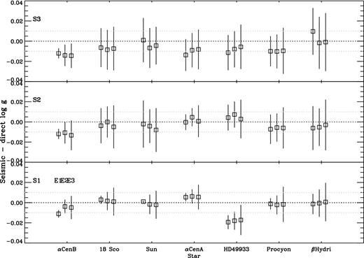
Accuracy of method. Seismic-minus-direct log g for the seven sample stars while considering different subsets of input observations (different panels, S1, S2, S3) and different observational errors (E1, E2, E3). See Section 3.3 for details.
Fig. 2 shows that for all observational sets and errors, log g is generally estimated to within 0.01 dex in accuracy and with a precision of 0.015 dex. This result clearly shows the validity of the global seismic quantities and atmospheric parameters for providing accurate values of log g. It can also be noted that the precision in log g typically decreases as (1) the observational errors increase (from E2 to E3), and (2) the information content decreases (S1 to S2 to S3, for example).
One noticeable result from Fig. 2 is the systematic offset in the derivation of log g for HD 49933 when we use [Fe/H] as input (S1). This could be due to an incorrect [Fe/H] or Teff, an error in the adopted direct log g or a shortcoming of the grid of models. This star is known to be active, and Mosser et al. (2005) found clear evidence of spot signatures in line bisectors. More recently, García et al. (2010) and Salabert et al. (2011) found frequency and amplitude variations similar to those in the Sun, evidence of the presence of a stellar cycle. García et al. (2010) derived an S-index of about 0.3 corresponding to a very active star, even though no detection of a magnetic field has yet been confirmed (Petit, private communication). Fabbian et al. (2012) showed that the magnetic effects in stellar models affect the determination of the metallicity and this, in turn, will affect the determination of other stellar parameters such as mass. In their work, they considered large magnetic field strengths of several hundreds of gauss.
Since no evidence of such a large magnetic field has yet been found for HD 49933, we propose another explanation. We consider the effect of the confirmed presence of spots on the effective temperature. By considering a spot area of about 20 per cent of the stellar surface we found that the real effective temperature (that of the non-spotted surface of the star) should increase by about 300 K with respect to the non-spotted star. Adding 300 K to Teff results in a seismic log g that increases by 0.011 dex for S1 (considering errors E1 and E2), which makes the new value consistent with the direct value within error bars. The increase of 0.011 dex corresponds to a relative increase of 3.7σ and 1.2σ for both error types E1 and E2. If we add this same 300 K for cases S2 and S3, we also find an increase in log g, but smaller (0.009 and 0.006 dex), corresponding to a relative increase of 0.6σ and 0.4σ, respectively.
3.5 Systematic errors in observations
For all of the calculations, we have assumed that the input observations are correct (accurate). While this is certainly more true for brighter nearby targets where high S/N data can be obtained, the same cannot be said for fainter stars. In particular with spectroscopic data, the determination of Teff and [Fe/H] are correlated and depend on the analysis methods used and the different model atmospheres (see e.g. Creevey et al. 2012a; Lebzelter et al. 2012). Additionally, for many stars a photometric temperature may be the only available one and while these estimates are very good, systematic errors are still unavoidable (Casagrande et al. 2010; Boyajian et al. 2012), in particular due to unknown reddenning. Larger photometric errors also lead to larger errors on the temperatures. This is not only a problem for fainter stars. For example, for β Hydri we found two determinations of Teff –an interferometric one and a spectroscopic one. For the spectroscopic Teff, the corresponding fitted metallicity from the atmospheric analysis will correlate with it.
To study the effect of systematic errors in the observations, we repeated our analysis for β Hydri while using three sets of input data that change only in Teff and [Fe/H]. The first set (1) uses the interferometric value of Teff from North et al. (2007) and their [Fe/H] (5872, −0.10), which we consider as the most correct, the second set (2) uses (5964, −0.10) and the third set (3) uses (5964, −0.03) as given by da Silva et al. (2006). The results for S1 and S2 are shown in Fig. 3. The lower panel shows that for a systematic error in both Teff and [Fe/H], the accuracy decreases. The top panel shows that when we only consider the Teff information, we get a smaller increase in the offset than when we consider both Teff and [Fe/H]. One way of interpreting this result is by considering that in S2 there is much more weight assigned to the seismic data than the atmospheric data, and so an incorrect atmospheric parameter should not influence the final result as much as in the case S1 where the atmospheric parameters have more weight. In the latter case, an incorrect Teff with the correct [Fe/H] will necessarily shift the mass either up or down (in terms of the H-R diagram), and result in a more displaced log g. However, in both cases, we see that the offset does not exceed 0.02 dex. For determining a seismic radius and mass, however, a systematic error in the input observations has a much more profound effect on the offset. In this case biases of the order of up to 6 and 20 per cent in radius and mass can be obtained (Creevey & Thévenin 2012). It must also be noted that a systematic error in the atmospheric parameters is going to have a much larger negative effect when we use only the global seismic quantities instead of performing a detailed seismic analysis with individual frequencies, where the latter have much more weight in the fitting process.
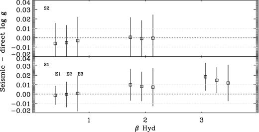
Seismic-minus-direct values of log g for β Hydri when the observations with systematic errors included for cases 2 and 3 are analysed by the seismic method. See Section 3.5.
3.6 Seismic determination of log g from the global seismic quantities for the reference stars
We summarize log g for the sample stars in Table 3 derived by radex10 using 〈Δν〉, νmax, Teff, and [Fe/H], and the true observational errors. We highlight the excellent agreement between our seismically determined parameters, and those obtained by direct mass and radius estimates. Log g is matched to within ∼0.01 dex, and 0.02 dex for HD 49933. We must also comment on the very small uncertainties given in Table 3; these results were obtained using the true (very small) observational errors given in Table 2 and typically one would not expect to obtain such small errors for fainter stars. As can be seen, the results using the relaxed observational errors give more reasonable parameter uncertainties, i.e. 0.010–0.015 dex, see Fig. 2, while still matching the direct log g to within 1σ.
4 DETERMINATION OF log g FOR AN EXTENDED LIST OF STARS
We apply our grid-based method to an extended list of stars with measured global seismic quantities and atmospheric parameters. Table 4 lists the star name along with the other measured parameters that are used as the input for our method. The first part of the table comprises primarily bright stars whose oscillation properties have been measured either from ground-based or spaced-based instrumentation (see references given in the table). For most of these stars, no errors are cited for 〈Δν〉 and νmax. The second part of the table lists a set of 22 solar-type stars observed by the Kepler spacecraft and studied in Mathur et al. (2012). We have taken the seismic and atmospheric data directly from this paper. To conduct a homogenous analysis of these stars, we adopted a 1.1 μHz error on 〈Δν〉 for all of the stars and a 5 per cent error on νmax, typical of what has been found for the large sample of Kepler stars (see Huber et al. 2011 and Section 5.1).
Measured seismic and atmospheric properties for an extended list of Sun-like oscillators.
| Star Name | 〈Δν〉 | νmax | Teff | [Fe/H] |
|---|---|---|---|---|
| (μHz) | (μHz) | (K) | (dex) | |
| HD 10700 | 169.0a | 4500a | 5383 ± 47a | −0.10 ± 0.07 |
| HD 17051 | 120.0b | 2700b | 6080 ± 80 | 0.15 ± 0.07 |
| HD 23249 | 43.8c | 700c | 4986 ± 57d | 0.15 ± 0.07 |
| HD 49385 | 55.8s | 1013s | 6095 ± 65s | +0.09 ± 0.05s |
| HD 52265 | 98.3 ± 0.1l | 1800l | 6100 ± 60l | 0.19 ± 0.05l |
| HD 61421 | 55.0 | 1000 | 6494 ± 48 | 0.01 ± 0.07 |
| HD 63077 | 97.0e | 2050e | 5710 ± 80 | −0.86 ± 0.07 |
| HD 102870 | 72.1f | 1400f | 6012 ± 64g | 0.12 ± 0.07 |
| HD 121370 | 39.9h | 750h | 6028 ± 47d | 0.24 ± 0.07 |
| HD 139211 | 85.0e | 1800e | 6200 ± 80 | −0.04 ± 0.07 |
| HD 160691 | 90.0i | 2000i | 5665 ± 80 | 0.32 ± 0.07 |
| HD 165341 | 161.7j | 4500j | 5300 ± 80 | 0.12 ± 0.07 |
| HD 170987 | 55.5 ± 0.8m | 1000m | 6540 ± 100m | −0.15 ± 0.06m |
| HD 181420 | 75.0n | 1500 ± 300n | 6580 ± 105o | 0.00 ± 0.06o |
| HD 181906 | 87.5 ± 2.6p | 1912 ± 47p | 6300 ± 150p | −0.11 ± 0.14p |
| HD 186408 | 103.1q | 2150q | 5825 ± 50q | 0.01 ± 0.03q |
| HD 186427 | 117.2q | 2550q | 5750 ± 50q | 0.05 ± 0.02q |
| HD 185395 | 84.0r | 2000r | 6745 ± 150r | -0.04r |
| HD 203608 | 120.4k | 2600k | 5990 ± 80 | −0.74 ± 0.07 |
| HD 210302 | 89.5e | 1950e | 6235 ± 80 | 0.01 ± 0.07 |
| KIC 3632418 | 60.63 ± 0.37 | 1110 ± 20 | 6150 ± 70 | −0.19 ± 0.07 |
| KIC 3656476 | 93.70 ± 0.22 | 1940 ± 25 | 5700 ± 70 | 0.32 ± 0.07 |
| KIC 4914923 | 88.61 ± 0.32 | 1835 ± 60 | 5840 ± 70 | 0.14 ± 0.07 |
| KIC 5184732 | 95.53 ± 0.26 | 2070 ± 20 | 5825 ± 70 | 0.39 ± 0.07 |
| KIC 5512589 | 68.52 ± 0.33 | 1240 ± 25 | 5710 ± 70 | 0.04 ± 0.07 |
| KIC 6106415 | 103.82 ± 0.29 | 2285 ± 20 | 5950 ± 70 | −0.11 ± 0.07 |
| KIC 6116048 | 100.14 ± 0.22 | 2120 ± 20 | 5895 ± 70 | −0.26 ± 0.07 |
| KIC 6603624 | 110.28 ± 0.25 | 2405 ± 50 | 5600 ± 70 | 0.26 ± 0.07 |
| KIC 6933899 | 72.15 ± 0.25 | 1370 ± 30 | 5830 ± 70 | −0.01 ± 0.07 |
| KIC 7680114 | 85.13 ± 0.14 | 1660 ± 25 | 5815 ± 70 | 0.10 ± 0.07 |
| KIC 7976303 | 50.95 ± 0.37 | 910 ± 25 | 6050 ± 70 | −0.52 ± 0.07 |
| KIC 8006161 | 148.21 ± 0.19 | 3545 ± 140 | 5340 ± 70 | 0.38 ± 0.07 |
| KIC 8228742 | 63.15 ± 0.32 | 1160 ± 40 | 6000 ± 70 | −0.15 ± 0.07 |
| KIC 8379927 | 120.86 ± 0.43 | 2880 ± 65 | 5960 ± 125 | −0.30 ± 0.07 |
| KIC 8760414 | 116.24 ± 0.56 | 2510 ± 95 | 5765 ± 70 | −1.19 ± 0.07 |
| KIC 10018963 | 55.99 ± 0.35 | 985 ± 10 | 6300 ± 65 | −0.47 ± 0.50 |
| KIC 10516096 | 84.15 ± 0.36 | 1710 ± 15 | 5900 ± 70 | −0.10 ± 0.07 |
| KIC 10963065 | 103.61 ± 0.41 | 2160 ± 35 | 6015 ± 70 | −0.21 ± 0.07 |
| KIC 11244118 | 71.68 ± 0.16 | 1405 ± 20 | 5705 ± 70 | 0.34 ± 0.07 |
| KIC 11713510 | 69.22 ± 0.20 | 1235 ± 15 | 5930 ± 52 | – |
| KIC 12009504 | 88.10 ± 0.42 | 1825 ± 20 | 6060 ± 70 | −0.09 ± 0.07 |
| KIC 12258514 | 74.75 ± 0.23 | 1475 ± 30 | 5950 ± 70 | 0.02 ± 0.07 |
References: All HD star measurements without references are taken from Bruntt et al. (2010); aTeixeira et al. (2009), bVauclair et al. (2008), cBouchy & Carrier (2003), dThévenin et al. (2005), eBruntt et al. (2010), fCarrier et al. (2005a), gNorth et al. (2009), hCarrier, Eggenberger & Bouchy (2005b), iBouchy et al. (2005), jCarrier & Eggenberger (2006), kMosser et al. (2008), lBallot et al. (2011), mMathur et al. (2010a), nBarban et al. (2009), oBruntt (2009), pGarcía et al. (2009), qMetcalfe et al. (2012), rGuzik et al. (2011), sDeheuvels et al. (2010). When 〈Δν〉 is not explicitly given it is calculated from the highest amplitude l = 0 modes. Values for the KIC stars are taken from Mathur et al. (2012).
Table 5 lists the derived value of log g and 2σ uncertainties (to allow for round-up error) for each of the stars using radex10. We show two values of log g; the first is obtained by using the four input constraints {〈Δν〉, νmax, Teff, [Fe/H]} and the second log gno[Fe/H] is obtained by omitting [Fe/H] from the analysis.
Derived seismic log g for an extended list of Sun-like oscillators. Log g and log gno[Fe/H] refer to using {〈Δν〉,νmax,Teff,[Fe/H]} and {〈Δν〉,νmax,Teff} as the constraints in the analysis. For a homogenous analysis we adopted 1.1 μHz and 5 per cent as the errors on 〈Δν〉 and νmax. We list 2σ uncertainties for log g.
| Star name | log g | log gno[Fe/H] |
|---|---|---|
| (dex) | (dex) | |
| HD 10700 | 4.55 ± 0.02 | 4.57 ± 0.02 |
| HD 17051 | 4.40 ± 0.02 | 4.39 ± 0.03 |
| HD 23249 | 3.81 ± 0.02 | 3.78 ± 0.04 |
| HD 49385 | 3.98 ± 0.02 | 3.97 ± 0.04 |
| HD 52265 | 4.28 ± 0.02 | 4.24 ± 0.02 |
| HD 61421 | 3.98 ± 0.02 | 3.97 ± 0.03 |
| HD 63077 | 4.22 ± 0.02 | 4.25 ± 0.03 |
| HD 102870 | 4.11 ± 0.02 | 4.10 ± 0.04 |
| HD 121370 | 3.82 ± 0.03 | 3.82 ± 0.03 |
| HD 139211 | 4.20 ± 0.02 | 4.21 ± 0.02 |
| HD 160691 | 4.22 ± 0.02 | 4.21 ± 0.02 |
| HD 165341 | 4.54 ± 0.02 | 4.54 ± 0.02 |
| HD 170987 | 3.98 ± 0.02 | 3.98 ± 0.03 |
| HD 181420 | 4.15 ± 0.02 | 4.15 ± 0.03 |
| HD 181906 | 4.22 ± 0.02 | 4.23 ± 0.02 |
| HD 186408 | 4.28 ± 0.02 | 4.28 ± 0.03 |
| HD 186427 | 4.36 ± 0.02 | 4.35 ± 0.03 |
| HD 185395 | 4.22 ± 0.02 | 4.23 ± 0.02 |
| HD 203608 | 4.35 ± 0.02 | 4.37 ± 0.04 |
| HD 210302 | 4.23 ± 0.02 | 4.24 ± 0.03 |
| KIC 3632418 | 4.00 ± 0.03 | 4.01 ± 0.04 |
| KIC 3656476 | 4.23 ± 0.02 | 4.23 ± 0.03 |
| KIC 4914923 | 4.21 ± 0.02 | 4.21 ± 0.03 |
| KIC 5184732 | 4.26 ± 0.02 | 4.25 ± 0.02 |
| KIC 5512589 | 4.05 ± 0.02 | 4.04 ± 0.04 |
| KIC 6106415 | 4.29 ± 0.02 | 4.30 ± 0.03 |
| KIC 6116048 | 4.25 ± 0.02 | 4.27 ± 0.03 |
| KIC 6603624 | 4.32 ± 0.02 | 4.32 ± 0.02 |
| KIC 6933899 | 4.09 ± 0.02 | 4.09 ± 0.04 |
| KIC 7680114 | 4.18 ± 0.02 | 4.17 ± 0.04 |
| KIC 7976303 | 3.89 ± 0.02 | 3.92 ± 0.04 |
| KIC 8006161 | 4.48 ± 0.02 | 4.48 ± 0.02 |
| KIC 8228742 | 4.02 ± 0.03 | 4.02 ± 0.04 |
| KIC 8379927 | 4.36 ± 0.02 | 4.40 ± 0.02 |
| KIC 8760414 | 4.31 ± 0.02 | 4.35 ± 0.03 |
| KIC 10018963 | 3.96 ± 0.03 | 3.96 ± 0.03 |
| KIC 10516096 | 4.17 ± 0.02 | 4.18 ± 0.03 |
| KIC 10963065 | 4.28 ± 0.02 | 4.29 ± 0.04 |
| KIC 11244118 | 4.09 ± 0.02 | 4.08 ± 0.03 |
| KIC 11713510 | 4.05 ± 0.04 | 4.05 ± 0.03 |
| KIC 12009504 | 4.21 ± 0.02 | 4.21 ± 0.03 |
| KIC 12258514 | 4.12 ± 0.02 | 4.12 ± 0.03 |
Fig. 4, top panel, compares the derived values of log g for the Kepler stars with those determined using the individual oscillation frequencies, as given by Mathur et al. (2012), with our 1σ error bars overplotted. We see that the grid-based method provides log g consistent with those derived from a detailed asteroseismic analysis, although a very small trend can be seen. For some of the stars they obtain a fitted initial He abundance significantly below the accepted primordial value, suggesting that the corresponding fitted mass and radius may be slightly biased (grey squares). If we omit these stars, then we fit a slope of −0.03 ± 0.02 to the difference between their and our log g values. White et al. (2011) and Mosser et al. (2013) point out that a discrepancy may exist between the two different theoretical values of 〈Δν〉 (using scaling relations or from individual frequencies), and the two different approaches could also be responsible for this trend. We see, however, that our values agree generally to within 0.01 dex. Silva Aguirre et al. (2012) have analysed six of these stars and the lower panel of Fig. 4 shows a comparison between their log g values with ours. Fitting the differences between our results, we obtain a slope of 0.001 ± 0.025 with a systematic offset of −0.003 ± 0.005, indicating no systematic trends.

5 PRECISION IN log g FOR A LARGE SAMPLE OF Kepler STARS OF CLASSES IV/V
Our primary objective was to test the accuracy of a seismic log g by using bright nearby targets that have independent mass and radius measurements. We showed in Section 3.4 (see Fig. 2) that our accuracy should be on a level of 0.01 dex with a precision of ∼0.02 dex using the set {〈Δν〉,νmax,Teff} for the small sample of stars covering the range 3.9 < log g < 4.6. In this section, we investigate the precision in log g for a sample of 403 V/IV stars (log g > 3.75) observed with the Kepler spacecraft by employing the same analysis methods. In particular, we pay attention to systematic errors by (1) using different sets of observational constraints, (2) comparing results using two different methods which incorporate different stellar evolution codes and physics, and (3) we also show the distribution of errors as a function of magnitude and log g and summarize the uncertainties and systematics as a function of magnitude.
5.1 Observations
During the first nine months of the Kepler mission targets to be monitored with a 1 min cadence during one month each were selected by the KASC.5 These stars were chosen based on information available in the Kepler Input Catalog, KIC, (Brown et al. 2011) and were expected to exhibit solar-like oscillations. A total of 588 stars with values of log g between 3.0 and 4.5 dex were analysed (García et al. 2011) and had their global seismic quantities determined (Chaplin et al. 2011; Huber et al. 2011; Verner et al. 2011). In this paper, we concentrate on a subset of 403 less-evolved stars with log g values between 3.75 and 4.50 dex derived from radex10, the range for which we have validated our method.
The global seismic quantities have been determined using the SYD pipeline as described by Huber et al. (2009), which uses the reference values of 〈Δν〉⊙ = 135.1 μHz and νmax⊙ = 3090 μHz. To avoid systematic errors (Chaplin et al.; in preparation), we adopted these same values in our grid. The uncertainties on the seismic quantities include a contribution from the scatter between different analysis pipelines (Verner et al. 2011, Chaplin et al. in preparation). Fig. 5 shows the cumulative distribution for the errors in the seismic observations, 〈Δν〉 (top) and νmax (bottom) in units of μHz and per cent, respectively, for the 403 stars. Our choice for absolute and relative errors is for consistency with units used in the recent literature. We show the cumulative distribution of the errors in order to see the typical errors for 50 and 80 per cent of the sample, which justifies the errors that we used in Section 3.3. These are less than 1.1/2.0 μHz for 〈Δν〉, and less than 5 per cent/8 per cent for νmax, respectively.
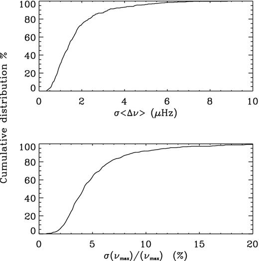
Cumulative distributions of the errors in 〈Δν〉 (top) and νmax (bottom) for 403 Kepler stars with derived log g between 3.75 and 4.5 dex. Data taken from Huber et al. (2011).
Teff derived by the KIC have been shown not to be accurate on a star-to-star basis (Molenda-Żakowicz et al. 2011), and so the ground-based Kepler support photometry (Brown et al. 2011) was re-analysed by Pinsonneault et al. (2012) to determine more accurate Teff for the ensemble of Kepler stars. These are the temperatures that we adopt for our first analysis and we refer to them as TeffPin. In their work. they consider a mean [Fe/H] = −0.20 ± 0.30 for all of the stars. Silva Aguirre et al. (2012) adapt an infrared flux method presented by Casagrande et al. (2010) for determining stellar temperatures. In their work, they apply this method to the large ensemble of Kepler stars to provide an alternative determination of Teff. We also adopt their Teff determinations in order to study the effect of biases in temperature estimates on the derived value of log g. We refer to these temperature estimates as Teffirfm. Support spectroscopic data have also been obtained for 93 of the stars and the metallicities are presented in Bruntt et al. (2012). We further include these data to study the effects of possible biases arising from lack/inclusion of metallicity information.
5.2 Seismic log g from different sets of observations
Using our validated method described in Section 3.2, we calculated values of log g and their uncertainties for the sample of 403 stars using the set of observations comprising {TeffPin,〈Δν〉,νmax} while adopting a mean [Fe/H] = –0.20 ± 0.30 dex. We refer to this set as the reference set. The distribution of the uncertainties as a function of log g is shown in Fig. 6. Here, it can be seen that typical uncertainties in log g for this set of 403 Kepler stars are below 0.02 dex (there is one star with an error of 0.05 dex), with a mean value of 0.015 dex.
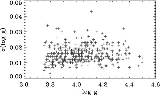
Distribution of uncertainties in log g σ(log g) as a function of log g for a sample of 403 Kepler stars, using radex10 with observational constraints comprising {TeffPin,〈Δν〉,νmax}.
In Fig. 7, we show the difference in the fitted log g while considering different input observational sets compared to the reference set ‘log gref’. The subsets are: Set 1 which considers 〈Δν〉 and TeffPin only and Set 2 which considers 〈Δν〉, νmax and Teffirfm. We note that for all of the analyses, [Fe/H] was constrained to −0.20 ± 0.30 dex, which corresponds to >90 per cent of the models of the grid.
![Differences in log g using subsets of observational constraints. The reference set comprises (〈Δν〉, νmax, TeffPin). Sets 1 and 2 comprise (〈Δν〉, TeffPin) and (〈Δν〉, νmax, TeffIR), respectively. For all sets [Fe/H] = −0.20 dex. The ±1σ error bars are average error bars measured over bins of 0.1 dex corresponding to Set X. See Section 5.2 for details.](https://oup.silverchair-cdn.com/oup/backfile/Content_public/Journal/mnras/431/3/10.1093/mnras/stt336/2/m_stt336fig7.jpeg?Expires=1750298672&Signature=I8lX08GLWc-IK1N1vDVZg7~a-Foxe7Oye2bBwXIv8yOUL5otpioo80mnkSONRTPw58rVtxNZ9A7GC20sysZ1ulp9w-xCzz4gzGxec1h7ESe-JQYuH3MoeP4PU0-nQNk9IFaxmEU-ZQ8cqmvhAoGXaU8y8tKKhp7Ifx0st9078ejm2HYJDXoKBhqmBIowDHi8CJCp4jnDGSAJoEzCn4lOwS35ctl1RxOUGHhsxuHfNylu0O0GRvytLAJ-fMYj5mQtw82ktaS5ZfABwaOTakSZSDugM~LA5pm73G11OSClNUTPSu57wyi2VTK6HyckapqTLp2BRf4hbb1eQ1kmjHSLUA__&Key-Pair-Id=APKAIE5G5CRDK6RD3PGA)
Differences in log g using subsets of observational constraints. The reference set comprises (〈Δν〉, νmax, TeffPin). Sets 1 and 2 comprise (〈Δν〉, TeffPin) and (〈Δν〉, νmax, TeffIR), respectively. For all sets [Fe/H] = −0.20 dex. The ±1σ error bars are average error bars measured over bins of 0.1 dex corresponding to Set X. See Section 5.2 for details.
Inspecting the top panel of Fig. 7 (Set 1), one can see that by omitting νmax as an observed quantity can result in differences of over 0.05 dex for a very small percentage of the stars, but the absolute difference between the full set of results is +0.005 dex with an rms of 0.01 dex. Here, we note that several authors have investigated the relation between 〈Δν〉 and νmax and find tight correlations (Bedding & Kjeldsen 2003; Stello et al. 2009a). The uncertainties arising from a set of data with less constraints usually increase and we indeed find an increase in the uncertainties σ of ∼0.01 dex. The extra scatter of 0.01 dex is taken care of in the larger σ.
Inspecting the lower panel of Fig. 7 (Set 2), one can see that the Teff derived by using different photometric scales results in a mean difference in log g of −0.002 dex (i.e. no significant overall effect) with an rms scatter of 0.007 dex. This latter fact implies that we can expect to add just under 0.01 dex to the error budget in log g by considering Teff derived from different methods. We found a similar result in Section 3.5 for β Hydri.
The mean value of the derived uncertainties (σ) in log g for Sets 1 and 2 are 0.023 and 0.015 dex, respectively, while those for the reference set are 0.015 dex. The accuracy of these log g (if we consider the reference set to be correct) is within a precision of 1σ.
Fig. 8 compares the derived log g using the reference set of observations to those with measured Teff and [Fe/H] from Bruntt et al. (2012). The absolute mean residual is 0.002 dex and is highlighted by the dotted grey line. We find that log g can differ by up to 0.02 dex by including [Fe/H]. This 0.02 dex is also consistent with what we found in Section 3.5 for β Hydri when we considered different metallicity constraints.
![Differences in the derived seismic log g from radex10 between adopting [Fe/H] = –0.20 ± 0.30 for all of the stars (log g) and adopting [Fe/H] from spectroscopic analyses by Bruntt et al. (2012), log g[Fe/H]. See Section 5.2 for details.](https://oup.silverchair-cdn.com/oup/backfile/Content_public/Journal/mnras/431/3/10.1093/mnras/stt336/2/m_stt336fig8.jpeg?Expires=1750298672&Signature=fchEi0qNR9Pj6B3SHoM7qIof6fyEzh2ecCyetLg5aJ-uCk29rEVOZDILFIRHKj9Iy9BndgrWMBvPu3UeUa50~8GWlQN7Fuzw8nhsdWziSao1fW2K5FFDfq21RqGIe478cPHZvqCpOgjyL1JCZOMkpBrQ09jDN~dDZ8wwUpEVQTKd2K-V6xPDd7gw8cgeRyH0DofyRYEwZj43SNBeOuz7SafhzY159USRkW2DLd6Dlddko42lrR1~yhX6qVU6TXOlZPyzRRKXpfvrlyH5-zgCWfBkU~Ke403a1PT1POWY1c~GbfTFc33gBzLJ1c~DgXP8v-Gof4VK9qYTXI8Un48tIQ__&Key-Pair-Id=APKAIE5G5CRDK6RD3PGA)
5.3 Comparison of results using different codes
To investigate the possible source of systematics arising from using a different evolution code and input physics, we determined log g using a second pipeline code, Yale–Bham (Gai et al. 2011; Creevey et al. 2012a). Details of the code can be found in the cited papers. Here, it suffices to know that the method is very similar to that of radex10, but the evolution code is based on yrec (Demarque et al. 2008) in its non-rotating configuration, with the following specifications: OPAL EOS (Rogers & Nayfonov 2002) and OPAL high-temperature opacities (Iglesias & Rogers 1996) supplemented with low-temperature opacities from Ferguson et al. (2005), and the NACRE nuclear reaction rates (Angulo et al. 1999). Diffusion of helium and heavy-elements were included, unlike radex10.
Fig. 9 shows the difference in the derived value of log g between radex10 and Yale–Bham using {〈Δν〉,νmax,TeffPin,[Fe/H] = −0.2}. We show the normalized difference, i.e. divided by the Yale–Bham errors, which are very similar to the radex10 errors. As can be seen from the figure, the agreement in log g between the different methods is within 1σ or <0.01 dex for 98 per cent of the stars and 2σ for all stars except one. A small absolute difference of 0.005 is found with an rms of 0.005 (in units of σ). This is most likely due to the different physics adopted in the codes. A very slight systematic trend is present with a slope of −0.005 ± 0.005. The agreement between the results using the different codes and methods is very encouraging. We can consider an upper limit of 0.01 dex as a typical systematic error arising from employing different codes.
The difference between the values of log g obtained by radex10 and Yale–Bham as a function of Radex10 log g and normalized by the Yale–Bham errors. See Section 5.3 for details.
5.4 Uncertainties and systematic errors in the seismic log g as a function of magnitude
In Fig. 10, we show the uncertainties in log g as a function of SDDS r magnitude (obtained from the KIC) while using the reference set of observations. As the figure shows, precision improves with apparent brightness, where more reliable measurements have smaller error bars. We can expect typical uncertainties in log g of less than 0.03 dex for the full sample with a mean value of <0.02 dex.
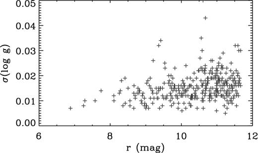
Distribution of derived uncertainties in the seismic log g from radex10 for 403 Kepler V/IV stars as a function of SDDS r magnitude.
In Table 6, we summarize for different apparent magnitude bins (1) the mean uncertainties 〈σ〉 and (2) the mean systematic errors 〈s〉 arising from adopting different temperature scales 〈sTeff〉, metallicities 〈s[Fe/H]〉 and different pipeline codes 〈scode〉. Note that the sample size for the bin with r < 9 is much smaller than the others and this is the reason we find a larger s[Fe/H] for r < 9. In the last row, we give the mean uncertainty and the adopted systematic errors over the full sample.
Summary of uncertainties σ and systematic errors s in the seismic log g from the Kepler sample of stars as a function of magnitude. We give the mean values 〈〉 of each over the sample that falls into the corresponding magnitude bin. The systematic errors s have subscripts which refer to possible sources of errors in the input Teff, [Fe/H], and the code that is used to generate the stellar models (see Sections 5.2 and 5.3 for details). In the final row, we summarize the mean uncertainties and adopted systematic errors for the full sample.
| r | 〈σ〉 | 〈sTeff〉 | 〈s[Fe/H]〉 | 〈scode〉 |
|---|---|---|---|---|
| (mag) | (dex) | (dex) | (dex) | (dex) |
| 6 < r <9 | 0.012 | 0.004 | 0.014 | 0.005 |
| 9 < r < 10 | 0.014 | 0.004 | 0.009 | 0.004 |
| 10 < r < 11 | 0.016 | 0.009 | – | 0.006 |
| 11 < r < 12 | 0.017 | 0.009 | – | 0.006 |
| 6 < r < 12 | 0.015 | 0.01 | 0.02 | 0.01 |
5.5 Summary of results for the sample of Kepler stars
From the sample of Kepler data with 3.75 < log g < 4.50 derived from seismic data, we obtain a mean precision σ of between 0.01 and 0.02 dex (max 0.03 dex for 99 per cent of stars) when 〈Δν〉, νmax and Teff are used as the input constraints for the pipeline analysis. A typical systematic error s of 0.01 dex can be added to account for a possible systematic error in Teff, such as that obtained by applying different calibration methods to photometry. Similarly, we can add a systematic error of 0.02 dex due to an incorrect or lack of an [Fe/H] measurement. We also showed that using different models and physics in the pipeline analyses yields results in log g consistent to within 0.01 dex, i.e. almost no model dependence.
Eliminating one of the seismic indices from the set of data yields a zero offset in the results for the full sample of stars and a typical scatter of 0.01 dex, although differences of over 0.05 dex were found for <1 per cent of the stars.
6 DISCUSSION
The first objective of this study was to investigate if we can determine log g reliably using global seismic quantities and atmospheric data. We showed that our method is reliable by comparing our results with values of log g derived from direct mass and radius estimates of seven bright nearby stars. We then applied our method to a list of 40 Sun-like stars and derived log g to within 1σ (∼0.01 dex) of those from Mathur et al. (2012) and Silva Aguirre et al. (2012). We also showed that for a sample of 400+ Kepler stars (6 < r mag < 12) with log g between 3.75 and 4.50 dex typical uncertainties σ of less than 0.02 dex can be expected and we estimated systematic errors s of no more than 0.04 dex arising from errors in Teff and [Fe/H] measurements and using different codes.
All of the Kepler stars will be observed by the Gaia mission, and for this reason they provide a valid set of calibration stars, by constraining log g with precisions and accuracies much better than spectroscopic or isochrone methods provide for the current list of calibration stars for Gaia. The astrophysical parameters to be determined from Gaia data using the astrometry, photometry and BP/RP spectrophotometry are Teff, AG, [Fe/H] and log g. By ensuring that the gsp_phot methods deliver log g consistent with the seismic value will reduce the uncertainties and inaccuracies in the other parameters. Moreover, an independent log g provides an extra constraint for the determination of the atmospheric parameters from gsp_spec where degeneracies between Teff and log g can inhibit the precision of atmospherically extracted parameters and chemical abundances.
While in this paper, we concentrated primarily on using Kepler data to determine log g, we note that both the CoRoT and Kepler fields have great potential in other aspects. For example, Miglio et al. (2012, 2013) determine distances, masses and ages of red giants from the CoRoT fields to constrain galactic evolution models, while Silva Aguirre et al. (2012) develop a method which couples asteroseismic analyses with the infrared flux method to determine stellar parameters including effective temperatures and bolometric fluxes (giving angular diameters), and hence distances. The distances obtained by both Miglio et al. (2013) and Silva Aguirre et al. (2012) can be compared directly with a Gaia distance for either calibration of Gaia data or stellar models. By combining data from CoRoT and Kepler with those from Gaia, we can also determine extremely precise angular diameters by coupling a seismically determined radius with the Gaia parallax. Finally, these stars will also be excellent calibrators for the FLAME workpackage of Gaia, which aims to determine masses and ages for one billion stars.
7 CONCLUSION
In this work, we explored the use of F, G, K IV/V stars observed in the Kepler field as a possible source of calibration stars for fundamental stellar parameters from the Gaia mission. Our first objective was to test the reliability/accuracy of a seismically determined log g, and using a sample of seven bright nearby targets, we proved that seismic methods are accurate (see Fig. 2) by obtaining results to within 0.01 dex of the currently accepted log g values. We showed, however, that the accuracy of the input atmospheric parameters does play a role in the accuracy of the derived parameters. For β Hydri, we found that errors in the atmospheric parameters, and in particular [Fe/H], can change log g by 0.02 dex.
We then applied our grid-based method radex10 to an extended sample of stars from the literature. We derived their seismic log g and these are given in Table 5. We showed that a grid-based log g is consistent with the values of log g obtained by detailed seismic analysis from Mathur et al. (2012) for 22 stars and in excellent agreement with the results from Silva Aguirre et al. (2012) for the 6 common stars. We find typical precisions in log g of 0.02 dex.
We finally studied the distribution of errors in log g from two analysis methods for a sample of 403 Kepler stars with 3.75 < log g < 4.5, and we obtained a typical uncertainty of between 0.01 and 0.02 dex in log g for F, G, K IV/V stars (see Table 6). We can add a total of 0.04 dex as a systematic error which arises from the adopted temperature scales (0.01 dex) and measured metallicities (0.02 dex) as well as the grids of models used (0.01 dex), which differ in evolution codes and input physics. The precisions in the data are unprecedented, and the systematic errors are much smaller than those stemming from any other method, especially for 7 < V < 12 stars (see e.g. Creevey et al. 2012a, fig. 1 and table 3 which compare spectroscopically derived log g for five Kepler stars with V ∼ 11).
As a final remark, we highlight that while there are >500 IV/V stars in the Kepler field and some in the CoRoT fields that exhibit Sun-like oscillations, there are also thousands of red giants in both CoRoT and Kepler fields with these same measured quantities, however, the accuracy of these stars’ seismic log g is yet to be studied.
OLC thanks Luca Casagrande and Victor Silva Aguirre for making data available. SB acknowledges NSF grant AST-1105930. AMS is supported in part by the European Union International Reintegration Grant PIRG-GA-2009-247732, the MICINN grant AYA2011-24704, by the ESF EUROCORES Program EuroGENESIS (MICINN grant EUI2009-04170), by SGR grants of the Generalitat de Catalunya and by the EU-FEDER funds. WJC and YE thank the UK STFC for grant funding to support asteroseismic research. MJPFGM acknowledges the support through research grant PTDC/CTE-AST/098754/2008, from FCT/MEC (Portugal) and FEDER (EC). OLC is a Henri Poincaré Fellow at the Observatoire de la Côte d’Azur (OCA), funded by OCA and the Conseil Général des Alpes-Maritimes.
For stars fainter than V ∼ 17, the radial velocities will not be available.
The G photometric scale is similar to V.
Kepler Asteroseismic Science Consortium, see http://astro.phys.au.dk/KASC/
