


Abstract
I present a systematic study of gamma-ray flares in blazars. For this purpose, I propose a very simple and practical definition of a flare as a period of time, associated with a given flux peak, during which the flux is above half of the peak flux. I select a sample of 40 brightest gamma-ray flares observed by Fermi Large Area Telescope during the first four years of its mission. The sample is dominated by four blazars: 3C 454.3, PKS 1510−089, PKS 1222+216 and 3C 273. For each flare, I calculate a light curve and variations of the photon index. For the whole sample, I study the distributions of the peak flux, peak luminosity, duration, time asymmetry, average photon index and photon index scatter. I find that (1) flares produced by 3C 454.3 are longer and have more complex light curves than those produced by other blazars; (2) flares shorter than 1.5 d in the source frame tend to be time asymmetric with the flux peak preceding the flare midpoint. These differences can be largely attributed to a smaller viewing angle of 3C 454.3 as compared to other blazars. Intrinsically, the gamma-ray emitting regions in blazar jets may be structured and consist of several domains. I find no regularity in the spectral gamma-ray variations of flaring blazars.
1 INTRODUCTION
Blazars constitute the most numerous class of permanent gamma-ray sources in the sky. In the 2-yr Fermi Large Area Telescope (LAT) Source Catalog (2FGL; Nolan et al. 2012), they constitute 67 per cent of associated point sources. They are characterized by strong and chaotic variability, occasionally producing spectacular flares. These events have attracted a considerable attention, triggering many extensive multiwavelength campaigns that attempted to characterize the overall behaviour of individual objects (e.g. Abdo et al. 2010b; Vercellone et al. 2010; Agudo et al. 2011; Ackermann et al. 2012; Hayashida et al. 2012). Unfortunately, the results of these campaigns vary widely, revealing relatively few consistent patterns that can be used to constrain the underlying physics of relativistic jets.
The Fermi Space Telescope offers a unique capability in the observational astronomy. Its main detector, LAT (Atwood et al. 2009), has a very wide field of view, of ∼50°. For most of its scientific mission starting in 2008 August, Fermi operated in the scanning mode, allowing a uniform coverage of the whole sky every several hours. Therefore, almost every blazar flare that happened during the Fermi mission was observed from the beginning to the end with basically the same sensitivity. It is then straightforward to produce a fairly complete and unbiased sample of gamma-ray flares of blazars, and to compare their properties within individual sources and between them. Such an approach has a potential to clearly demonstrate the similarities and differences among individual blazar flares.
In this work, I study a sample of 40 bright gamma-ray flares of blazars detected by Fermi/LAT during the first four years of its mission. In Section 2, I propose a useful definition of a gamma-ray flare, and describe the process of selecting the sample. In Section 3, I present light curves of these flares, and study the distributions of their duration, time asymmetry, average photon index and photon index scatter. In Section 4, I discuss the general properties of the flares and their interpretation. I conclude in Section 5.
2 SAMPLE SELECTION
Any discussion of blazar flares immediately leads to a fundamental difficulty – how to define a flare. The nature of blazars variability is stochastic (Abdo et al. 2010c), characterized by a very high duty cycle, and there is no consistent ‘background’ flux level. It is thus difficult to draw a division between ‘flares’ and ‘quiescence’. In fact, many researchers question the validity of using the term ‘flare’ in the context of blazar light curves. On the other hand, this term is intuitive, as blazars spend very little time in their highest flux states (Tavecchio et al. 2010). My opinion is that the term is certainly useful, but for a systematic study a rigorous definition is necessary.
Here, I propose a very simple definition, in which a flare is a contiguous period of time, associated with a given flux peak, during which the flux exceeds half of the peak value, and this lower limit is attained exactly twice – at the beginning and at the end of the flare. One can show that this definition does not allow any two flares to overlap. Every two flares must be separated by a flux minimum which is lower than half of the lower peak. A flare may include minor peaks, but they are not considered to be peaks of separate subflares. This definition is natural in a stochastic light curve with a power density spectrum in the form of a power law, as it is based on equal flux ranges on a logarithmic scale. It is practical, as it is very easy to determine local flux peaks and the associated lower flux limits. Also, it automatically provides two standard variability time-scales often discussed in the blazar studies – the flux-doubling time-scale and the flux-halving time-scale. Fig. 1 illustrates this definition in various real light curves.
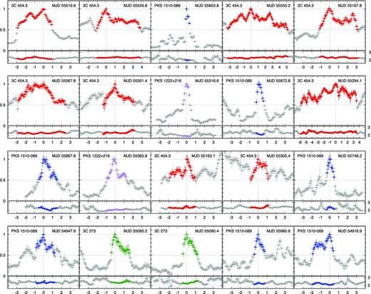
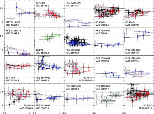
Light curves of individual gamma-ray flares calculated from the Fermi/LAT data, presented in the order of descending peak photon flux density. For each flare, the upper panel shows the normalized photon flux density integrated in the energy range 0.1–300 GeV in 0.5-d time intervals with a 0.1-d step, and the lower panel shows the corresponding photon index. The horizontal axes show time in days measured relative to the flare peak. The data points belonging to the flare period are highlighted with colours.

– continued
The process of selecting a flux-limited sample of blazar flares is divided into two steps. In the first step, a preliminary list of blazar active periods is extracted from the Fermi/LAT Monitored Source List.1 It is a data base of daily and weekly flux estimates for all sources exceeding the |$0.1\text{--}300\;{\rm GeV}$| photon flux of 10−6 ph s−1 cm−2. I select all daily photon fluxes during the first four years of the Fermi mission (MJD 54682–56143) above 3 × 10⁻⁶ ph s−1 cm−2 for sources located away from the Galactic plane (|b| > 10°). For each blazar, these daily entries are grouped into active periods, which are separated by gaps of at least 10 d. If an active period contains two flux peaks separated by at least 10 d and a flux minimum lower than the half of the lower peak flux or at least one-day gap, it is split into two active periods along the flux minimum. The active periods for all blazars are sorted according to the decreasing peak flux, and the first 30 active periods are selected for the second step. This choice corresponds to a minimum flux peak of 4.5 × 10⁻⁶ s−1 cm−2, and the preliminary list of active periods consists of six blazars: 3C 454.3, PKS 1510−089, PKS 1222+216, 3C 273, PKS 0402−362 and PKS 1329−049.
In the second step, I perform the maximum likelihood analysis of the Fermi/LAT data. I use the standard analysis software package science tools v9r27p1, with the instrument response function P7SOURCE_V6, the Galactic diffuse emission model gal_2yearp7v6_v0 and the isotropic background model iso_p7v6source. Events of the SOURCE class were extracted from regions of interest of 10° radius centred on the position of each blazar. The background models included all sources from the 2FGL within 15°, their spectral models are power laws with the photon index fixed to the catalogue values. I checked the raw count maps for any new source not included in the 2FGL. In the case of PKS 1510−089, the source model included TXS 1530−131 (Gasparrini & Cutini 2011). I selected events in the energy range between 100 MeV and 300 GeV. The spectra of all studied blazars were modelled with power laws. I used overlapping time bins, with the shift between consecutive bins equal to 1/5 of the bin lengths. This allows us to avoid the dependence of the results on the ‘phase’ of the time bins and provides a natural interpolation of the light curve. While the consecutive flux measurements are not entirely independent, this is not a problem for the subsequent analysis of the flare parameters.
Light curves calculated with different time bins reveal different amounts of detail, which affects the classification of certain events as flares, and the flares parameters. The shorter time bins reveal more details and potentially shorter flares, but limited photon statistics determines the size of the sample of flares that can be studied reliably. The brightest gamma-ray flares (>10−5 ph s−1 cm−2) can be probed once per orbital period of the Fermi satellite (∼1.5 h; Foschini et al. 2011). Here, I decide to use the time bin length of 0.5 d, with the shifts of 0.1 d, always starting from a full modified julian day (MJD).
Systematic analysis of all candidate active periods revealed that some of them consist of a few flares, so that the list of all flares revealed by this analysis exceeds 50 entries. From this, I select the final list of the 40 brightest flares, which corresponds to the minimum peak flux of 7.1 × 10⁻⁶ ph s−1 cm−2. This limiting peak flux value corresponds roughly to the peak of a histogram of the logarithmic peak flux distribution of all identified flares. The final list of brightest gamma-ray blazar flares is reported in Table 1. For each flare, I calculate the flux-doubling time t1, the flux-halving time t2 and the total flare duration T = t1 + t2. I also calculate the time asymmetry parameter k = (t1 − t2)/(t1 + t2), which can take values between −1 and 1, with k = 0 corresponding to a time-symmetric flare (t1 = t2); the average photon index Γ (NE ∝ E−Γ) and the root mean square (rms) of deviations of the photon index from the mean value. Individual flares will be referred to using their row number in Table 1.
List of the brightest gamma-ray flares of blazars. MJDpeak is the moment of flux peak, Fpeak is the peak flux in units of 10−6 ph s−1 cm−2, t1 is the flux-doubling time-scale, t2 is the flux-halving time-scale, T = (t1 + t2) is the flare duration, k = (t1 − t2)/(t1 + t2) is the time asymmetry parameter, 〈Γ〉 is the average photon index, and rms(Γ) is the photon index scatter. All times are in units of days. References: (a) Abdo et al. (2011), (b) Ackermann et al. (2010), (c) Tanaka et al. (2011), (d) Abdo et al. (2010b) and (e) Abdo et al. (2010a).
| # | Blazar | MJDpeak | Fpeak | t1 | t2 | T | k | 〈Γ〉 | rms(Γ) | Reference |
|---|---|---|---|---|---|---|---|---|---|---|
| 1 | 3C 454.3 | 55520.0 | 77.2 ± 2.4 | 2.9 | 1.0 | 3.9 | 0.49 ± 0.07 | 2.24 | 0.10 | a |
| 2 | 3C 454.3 | 55526.9 | 33.3 ± 1.8 | 1.1 | 3.9 | 5.0 | −0.58 ± 0.05 | 2.32 | 0.04 | |
| 3 | PKS 1510−089 | 55853.8 | 26.6 ± 2.0 | 0.2 | 0.4 | 0.6 | −0.45 ± 0.46 | 1.99 | 0.03 | |
| 4 | 3C 454.3 | 55550.3 | 23.6 ± 1.3 | 3.2 | 5.1 | 8.3 | −0.23 ± 0.03 | 2.32 | 0.09 | |
| 5 | 3C 454.3 | 55167.8 | 21.8 ± 1.5 | 1.2 | 3.1 | 4.3 | −0.44 ± 0.06 | 2.32 | 0.07 | b |
| 6 | 3C 454.3 | 55567.8 | 19.2 ± 1.6 | 2.9 | 2.5 | 5.4 | 0.07 ± 0.05 | 2.29 | 0.08 | |
| 7 | 3C 454.3 | 55301.5 | 16.4 ± 1.8 | 1.3 | 2.2 | 3.5 | −0.26 ± 0.07 | 2.35 | 0.13 | |
| 8 | PKS 1222+216 | 55316.6 | 15.6 ± 0.9 | 0.4 | 0.4 | 0.8 | 0.00 ± 0.31 | 1.89 | 0.03 | c |
| 9 | PKS 1510−089 | 55872.8 | 15.3 ± 1.2 | 0.2 | 0.7 | 0.9 | −0.56 ± 0.29 | 2.13 | 0.08 | |
| 10 | 3C 454.3 | 55294.1 | 15.3 ± 0.8 | 5.9 | 3.6 | 9.5 | 0.24 ± 0.03 | 2.37 | 0.10 | b |
| 11 | PKS 1510−089 | 55867.8 | 14.2 ± 1.5 | 0.5 | 1.5 | 2.0 | −0.50 ± 0.13 | 2.21 | 0.13 | |
| 12 | PKS 1222+216 | 55365.8 | 14.2 ± 1.0 | 1.0 | 1.3 | 2.3 | −0.16 ± 0.11 | 2.07 | 0.05 | c |
| 13 | 3C 454.3 | 55163.1 | 11.8 ± 1.4 | 2.0 | 1.0 | 3.0 | 0.33 ± 0.08 | 2.34 | 0.09 | |
| 14 | 3C 454.3 | 55305.5 | 11.1 ± 1.5 | 0.8 | 1.1 | 1.9 | −0.16 ± 0.13 | 2.38 | 0.12 | |
| 15 | PKS 1510−089 | 55746.2 | 11.1 ± 1.4 | 0.4 | 0.5 | 0.9 | −0.11 ± 0.27 | 2.30 | 0.12 | |
| 16 | PKS 1510−089 | 54948.0 | 10.6 ± 2.3 | 0.9 | 1.3 | 2.2 | −0.18 ± 0.11 | 2.38 | 0.08 | d |
| 17 | 3C 273 | 55095.3 | 10.3 ± 0.9 | 0.4 | 1.6 | 2.0 | −0.60 ± 0.13 | 2.42 | 0.10 | e |
| 18 | 3C 273 | 55090.5 | 10.2 ± 0.9 | 0.4 | 1.2 | 1.6 | −0.50 ± 0.16 | 2.37 | 0.12 | e |
| 19 | PKS 1510−089 | 55980.6 | 10.0 ± 1.3 | 0.5 | 0.8 | 1.3 | −0.23 ± 0.19 | 2.24 | 0.07 | |
| 20 | PKS 1510−089 | 54917.0 | 9.9 ± 0.7 | 1.9 | 0.5 | 2.4 | 0.58 ± 0.11 | 2.20 | 0.09 | d |
| 21 | PKS 1510−089 | 55851.9 | 9.9 ± 1.0 | 0.2 | 0.5 | 0.7 | −0.38 ± 0.39 | 2.32 | 0.13 | |
| 22 | 3C 454.3 | 55195.2 | 9.7 ± 0.8 | 0.6 | 1.6 | 2.2 | −0.45 ± 0.12 | 2.28 | 0.06 | b |
| 23 | PKS 1222+216 | 55310.7 | 9.6 ± 0.8 | 0.5 | 0.7 | 1.2 | −0.22 ± 0.21 | 1.98 | 0.08 | c |
| 24 | 3C 454.3 | 55323.5 | 9.1 ± 0.9 | 4.2 | 1.8 | 6.0 | 0.40 ± 0.04 | 2.38 | 0.10 | |
| 25 | 3C 454.3 | 55327.2 | 8.8 ± 1.2 | 1.9 | 1.2 | 3.1 | 0.23 ± 0.08 | 2.33 | 0.08 | |
| 26 | 3C 273 | 55202.9 | 8.7 ± 1.1 | 0.3 | 0.6 | 0.9 | −0.33 ± 0.28 | 2.45 | 0.09 | |
| 27 | PKS 1222+216 | 55342.1 | 8.7 ± 0.8 | 0.8 | 0.8 | 1.6 | −0.03 ± 0.16 | 1.93 | 0.10 | |
| 28 | PKS 1510−089 | 55990.8 | 8.5 ± 0.7 | 5.2 | 1.1 | 6.3 | 0.65 ± 0.04 | 2.29 | 0.08 | |
| 29 | PKS 1510−089 | 55983.1 | 8.4 ± 0.8 | 0.5 | 0.4 | 0.9 | 0.11 ± 0.27 | 2.19 | 0.04 | |
| 30 | PKS 1510−089 | 54961.8 | 8.2 ± 0.7 | 0.3 | 0.3 | 0.6 | 0.00 ± 0.41 | 2.59 | 0.12 | d |
| 31 | 3C 454.3 | 55214.3 | 8.0 ± 0.9 | 0.8 | 0.8 | 1.6 | 0.03 ± 0.16 | 2.42 | 0.05 | |
| 32 | PKS 1510−089 | 56002.4 | 7.8 ± 1.0 | 1.8 | 0.9 | 2.7 | 0.32 ± 0.09 | 2.45 | 0.11 | |
| 33 | 3C 454.3 | 55154.8 | 7.8 ± 0.9 | 0.5 | 1.9 | 2.4 | −0.58 ± 0.11 | 2.35 | 0.13 | |
| 34 | PKS 1510−089 | 55767.6 | 7.6 ± 0.8 | 0.4 | 0.5 | 0.9 | −0.11 ± 0.27 | 2.09 | 0.07 | |
| 35 | PKS 1222+216 | 55377.5 | 7.6 ± 0.7 | 0.4 | 1.1 | 1.5 | −0.45 ± 0.17 | 2.18 | 0.06 | |
| 36 | 3C 454.3 | 55283.9 | 7.6 ± 1.1 | 1.3 | 1.4 | 2.7 | −0.04 ± 0.09 | 2.37 | 0.13 | |
| 37 | PKS 1510−089 | 55876.1 | 7.4 ± 0.8 | 0.7 | 1.0 | 1.7 | −0.18 ± 0.14 | 2.29 | 0.07 | |
| 38 | PKS 1222+216 | 55234.0 | 7.4 ± 0.8 | 0.7 | 0.4 | 1.1 | 0.27 ± 0.23 | 2.25 | 0.02 | |
| 39 | PKS 0402−362 | 55827.5 | 7.3 ± 1.0 | 0.3 | 1.8 | 2.1 | −0.71 ± 0.13 | 2.27 | 0.11 | |
| 40 | 3C 454.3 | 55091.6 | 7.1 ± 0.8 | 4.4 | 1.1 | 5.5 | 0.60 ± 0.05 | 2.42 | 0.13 |
Very short flares (e.g. flare #3 – PKS 1510−089 at MJD 55854) indicate that the measured flux can change significantly over a single time bin shift of δt = 0.1 d. This provides a practical estimate of accuracy in determining the moments of flare beginning, peak and ending. The uncertainty of parameters t1, t2 and T can be estimated as |$\sqrt{2}\delta t = 0.14\;{\rm d}$|. The uncertainty of the asymmetry parameter k is given by δk = [2(3 + k2)]1/2(δt/T), which is large for the shortest flares. The values of δk are reported in Table 1.
3 RESULTS
My sample of the brightest gamma-ray flares of blazars reported in Table 1 is produced by only five blazars: 3C 454.3 (16 entries), PKS 1510−089 (14 entries), PKS 1222+216 (6 entries), 3C 273 (3 entries) and PKS 0402−362 (1 entry). Remarkably, 3C 454.3 produced 7 of the 10 brightest flares. About 20 flares exceed the peak flux level of 10−5 ph s−1 cm−2.
In the following analysis, I will compare both the observed parameters and parameters measured in the source frame. The redshifts and luminosity distances of the five blazars that produced the sample are given in Table 2.
Redshifts and luminosity distances of blazars producing the sample of brightest gamma-ray flares. I adopt standard ΛCDM cosmology with H0 = 71 km s−1 Mpc−1, Ωm = 0.27 and ΩΛ = 0.73.
| Blazar | z | dL [Gpc] |
|---|---|---|
| 3C 454.3 | 0.859 | 5.49 |
| PKS 1510−089 | 0.360 | 1.92 |
| PKS 1222+216 | 0.432 | 2.37 |
| 3C 273 | 0.158 | 0.75 |
| PKS 0402−362 | 1.423 | 10.31 |
| Blazar | z | dL [Gpc] |
|---|---|---|
| 3C 454.3 | 0.859 | 5.49 |
| PKS 1510−089 | 0.360 | 1.92 |
| PKS 1222+216 | 0.432 | 2.37 |
| 3C 273 | 0.158 | 0.75 |
| PKS 0402−362 | 1.423 | 10.31 |
3.1 Light curves
Fig. 1 shows normalized light curves and photon index variations of all 40 flares, in the order of decreasing peak flux, the same as in Table 1. The data points belonging to the flare period are highlighted with a colour. One can immediately notice a great variety of the flare shapes and durations. Looking only at the first 10 panels, it is striking that the flares produced by 3C 454.3 appear very different from those produced by PKS 1510−089 and PKS 1222+216 – the former are longer and more complex than the latter. However, looking at the next 30 panels, the picture is less clear. Many flares, especially the longest ones, are characterized by a complex structure with multiple peaks separated by shallow minima. The time-scale of these substructure is comparable to the time-scale of short flares characterized by a single peak. Medium-long flares (T ∼ 2 d) often show a single substructure following the main peak (e.g., flare #12 – PKS 1222+216 at MJD 55366), and sometimes preceding the main peak (e.g., flare #20 – PKS 1510−089 at MJD 54917). This results in the significant time asymmetry of these flares.
3.1.1 Flare duration
In order to further investigate the temporal properties of blazar flares, in Fig. 2, I plot the distribution of the flare duration versus peak flux. Flare durations span the range between 0.5 and 10 d. The lower limit corresponds to the time bin length, and the number of flares with T < 1 d (9) is the same as that of flares with 1 d ≤ T < 2 d. While the sample might be somewhat incomplete for T < 1 d, it is not likely for longer flares. The average flare duration is 2.7 d, and the median is 2.1 d. There appears to be no general trend between the flare duration and the peak flux. However, there is a significant difference between 3C 454.3 on one hand and PKS 1510−089, PKS 1222+216 and 3C 273 on the other. Flares produced by 3C 454.3 are on average longer than those produced by other blazars. 3C 454.3 did not produce a flare shorter than 1.6 d, while other blazars generally produced flares shorter than 3 d, with the sole exception of flare #28 (PKS 1510−089 at MJD 55991). For the peak flux greater than 1.2 × 10⁻⁵ ph s−1 cm−2, there is a complete separation of the two groups. Also, there is no discernible difference between the distributions of flares produced by PKS 1510−089, PKS 1222+216 and 3C 273.
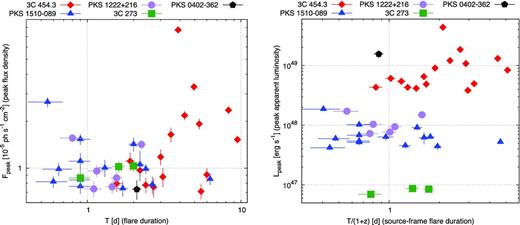
Left panel: distribution of the observed flare duration T versus the peak flux density Fpeak. Right panel: distribution of the source-frame flare duration T/(1 + z) versus the peak apparent luminosity Lpeak. The shape and colour of each point indicate the host blazar.
Also in Fig. 2, I plot the distribution of the source-frame flare duration versus peak apparent luminosity. I do not use luminosity integrated from the power-law spectral fit in the 0.1–300 GeV range, because: (1) the corresponding source-frame energy range depends on the source redshift, (2) the gamma-ray spectra of these blazars are actually curved/broken, so the power-law spectral fits overestimate the bolometric luminosity above a few GeV. Instead, I use the νLν value corresponding to the source-frame photon energy of 500 MeV. Apparent luminosities of the brightest blazar flares span three orders of magnitude, mainly due to the differences in luminosity distances between the sources. The flare produced by PKS 0402−362, while 39th in observed photon flux, is 3rd in apparent luminosity, due to the high source redshift. There is no clear trend between flare luminosity and duration.
3.1.2 Flare asymmetry
Furthermore, insight into the flare profiles can be gained by looking at the time asymmetry parameter k. In Fig. 3, I plot the distribution of the source-frame flare duration T/(1 + z) versus k. The values of k range between −0.7 and 0.7. This means that the observed flares do not show a very rapid onset directly to the peak or a very rapid decay directly from the peak. The average value of k is −0.1, and the median is −0.16. Therefore, there is a slight tendency for the flux-doubling time t1 to be shorter than the flux-halving time t2. Fig. 3 reveals a significant difference between short and long flares. Flares shorter than ∼1.5 d in the source frame have predominantly negative k, while flares longer than ∼1.5 d have a broad and roughly uniform distribution of k. Individual blazars produce flares of different distributions of k, which can be largely understood as resulting from different distributions of the flare durations. 3C 454.3 produces flares of a broad distribution of k, with four out of the five shortest flares characterized by negative k. PKS 1510−089 produces flares with mostly negative k; however, the three longest flares have significantly positive values of k. PKS 1222+216 produces fairly symmetric flares, while the three flares produced by 3C 273 have significantly negative k. The most asymmetric flare in the sample is the one produced by PKS 0402−362. There is a slight trend for the brighter flares to have more negative values of k; the average value of k for the 20 brightest flares is −0.16.
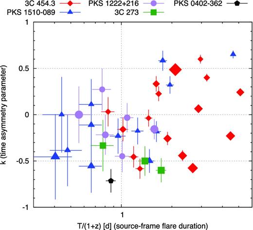
Distribution of the source-frame flare duration T/(1 + z) versus the time asymmetry parameter k. The shape and colour of each point indicate the host blazar, and the point size is proportional to the logarithm of peak flux Fpeak.
3.2 Spectral variations
In order to study variations of the photon index in detail, in Fig. 4, I show scatter plots of the normalized flux density Fpeak versus the photon index Γ for each flare in the sample. Varying point intensity is used to show the flow of time. It is clear that individual flares are characterized by different average values of the photon index, and also by different spreads of its values. Scatter plots for long flares are obviously more complex than those for short flares. In some cases, the spectral evolution of the gamma-ray flare takes the form of a clear loop (e.g. flare #11 – PKS 1510−089 at MJD 55868). Such loops were observed numerously in blazars in gamma-rays (e.g. Ackermann et al. 2010) and X-rays (e.g. Fossati et al. 2000). The most basic characteristic of a loop is its orientation in time. In Fig. 4, clockwise (CW) loops correspond to spectral hardening (decreasing Γ) at the peak, and counterclockwise (CCW) loops correspond to spectral softening (increasing Γ). I can identify clear cases of CW loops (flares #8, #9, #11) and CCW loops (flares #23, #26, #30). However, most cases are difficult to classify, and thus I cannot draw a definite conclusion about the statistics of loop orientations.
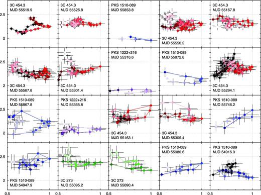
Scatter plots showing the normalized |$0.1\text{--}300\;{\rm GeV}$| photon flux (horizontal axes) versus the corresponding photon index (vertical axes) for individual flares. The intensity of data points indicates the time flow from dark to bright.
– continued
3.2.1 Average photon index
In Fig. 5, I plot the distribution of the source-frame flare duration T/(1 + z) versus average photon index 〈Γ〉. The average photon index takes values between 1.9 and 2.6. The extreme values are realized only by very short flares, with (1 + z)T ≲ 1 d, and for long flares the range of 〈Γ〉 converges to the vicinity of 2.3–2.4. The average value of 〈Γ〉 for the sample is 2.27, and the median is 2.3. Individual blazars produce flares of significantly different distributions of 〈Γ〉. 3C 454.3 produces flares characterized by 2.2 < 〈Γ〉 < 2.45, i.e. with a hardness typical for the whole sample and with a very small scatter. PKS 1510−089 produces flares with a wide range of average photon index, 2 ≲ 〈Γ〉 ≲ 2.6. PKS 1222+216 produces relatively hard flares, with 1.9 ≲ 〈Γ〉 ≲ 2.25, and 3C 273 produces relatively soft flares, with 〈Γ〉 ∼ 2.4. There is no clear dependence between the peak flux density Fpeak and the average photon index.
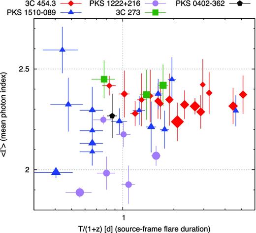
Distribution of the source-frame flare duration T/(1 + z) versus the average photon index 〈Γ〉. The shape and colour of each point indicate the host blazar, and the point size is proportional to the logarithm of peak flux density Fpeak.
3.2.2 Photon index scatter
In Fig. 6, I plot the distribution of the average photon index 〈Γ〉 versus the photon index scatter rms(Γ). The maximum value of the photon index scatter is ∼0.13, and the minimum value is ∼0.02. The average and median values are ∼0.09. I find the general trend that the photon index scatter is higher for softer flares (higher 〈Γ〉), Pearson's correlation coefficient is ρ(〈Γ〉, rms(Γ)) = 0.5. Individual blazars show a large range of rms(Γ) values. Flares of PKS 1222+216 are characterized by low photon index scatter (rms(Γ) < 0.1), while flares of 3C 273 show high average (rms(Γ) > 0.09). Flares of duration longer than 0.9 d in the source frame generally have rms(Γ) ≳ 0.05, but the high photon index scatter values (rms(Γ) > 0.1) are exhibited by both long and short flares.
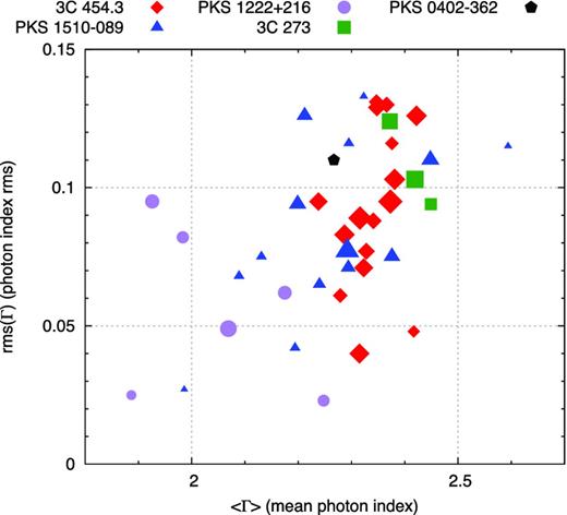
Distribution of the average photon index 〈Γ〉 versus the photon index scatter rms(Γ). The shape and colour of each point indicate the host blazar, and the point size is proportional to the logarithm of source-frame flare duration T/(1 + z).
4 DISCUSSION
Variability of blazars is a stochastic phenomenon, regardless of in which band and at what time-scales it is studied. Even the very notion of a flare, while intuitive, is controversial, because it is difficult to formulate a simple and practical definition. Here, I propose a simple mathematical definition of a flare, based on the peak and half-peak flux levels, without considering the complexity of the observed light curves. Such defined flare may be fairly simple, with a single roughly time-symmetric peak, or complex, with several local maxima and minima. In practice, even such a simple definition of a flare faces some problems: the flare duration and peak flux depend on the sampling (in the case of Fermi/LAT data, the time binning), and limited photon statistics introduces some ambiguity in determining the flare beginning and end. Nevertheless, using the same definition for a uniform sample of blazar flares reveals new information about the variability of blazars.
The focus of this study is on individual flares hosted by a handful of blazars. Flares of any given blazar, separated by months or years, can be considered independent phenomena, as they are produced in constantly flowing relativistic jets. Any similarities and differences between them reflect independent realizations of the underlying processes of energy dissipation and particle acceleration. Similarities and differences between flares produced in different blazars reflect the environmental factors that vary over time-scales of many years.
4.1 Temporal properties
The most appealing finding of this study is the systematic difference between flares produced by 3C 454.3 and other bright blazars. Flares produced by 3C 454.3 are significantly longer and more complex. A brief look at the first 10 panels of Fig. 1 shows that they are characterized by multiple secondary maxima and minima. In accordance with the adopted definition of the flare, these minima are always higher than half of the peak flux for a given flare. The light curve of 3C 454.3 can be contained in a limited range of flux values for several days. Other blazars can produce such long flares only occasionally (e.g., flare #28 in PKS 1510−089). The long flares of 3C 454.3 can be described as a collection of closely spaced simple flares of comparable peak flux levels. On the other hand, short flares displayed mostly by other blazars appear to be simple (3C 454.3 can also produce simple flares, e.g. flare #31).
The distinct structure of flares produced systematically by 3C 454.3 could be explained by its special jet orientation. (Hovatta et al. 2009) provide estimates of the jet Lorentz factor Γj = (1 − β2j)− 1/2, where βj = vj/c, and viewing angle θobs for a large sample of blazars monitored in the MOJAVE programme. They estimate the viewing angle of 3C 454.3 at θobs ≃ 1| ${.\!\!\!\!\!\!^{\circ}}$|3 ≃ 0.45Γ− 1j, which is significantly smaller than the values for PKS 1510−089 (3| ${.\!\!\!\!\!\!^{\circ}}$|4), PKS 1222+216 (5| ${.\!\!\!\!\!\!^{\circ}}$|1) and 3C 273 (3| ${.\!\!\!\!\!\!^{\circ}}$|3). The corresponding Doppler factor for 3C 454.3, |$\mathcal {D} = [\Gamma _{\rm j}(1-\beta _{\rm j}\cos \theta _{\rm obs})]^{-1}\simeq 33\simeq 1.7\Gamma _{\rm j}$|, is the highest among the blazars producing the brightest gamma-ray flares. This explains why 3C 454.3, at z = 0.86, being more distant than other blazars, is the brightest of them. In fact, the viewing angle of the inner jet of 3C 454.3 could be even smaller than that estimated from the very long baseline interferometry (VLBI) studies, as these estimates by their nature are not very precise, and the jets may be slightly bent even at parsec scales (Hough et al. 2002). The observed emission from a jet element propagating at the Doppler factor |$\mathcal {D}$| is boosted by factor |$\mathcal {D}^4$|. For θobs = 0 we have |$\mathcal {D}=(1+\beta _{\rm j})\Gamma _{\rm j}$|, while for θobs = Γ− 1j (Doppler cone) we have |$\mathcal {D}=\Gamma _{\rm j}$|. The difference in the Doppler factors by factor (1 + βj) ≃ 2 corresponds to a difference in the observed fluxes by factor ≃ 16. For an average blazar, one can expect that θobs ∼ θj ∼ Γ− 1j, where θj is the jet half-opening angle, so that the observer is located at random orientation within the Doppler cone.2 In such a case, only a fraction of the jet volume is strongly Doppler boosted and effectively contributes to the observed emission (see Fig. 7). However, when θobs ≪ θj, most of the jet volume is strongly Doppler boosted. If individual simple flares are produced in different parts of the jet cross-section, their Doppler factors will be very similar, resulting in similar peak fluxes. Thus, the long complex gamma-ray flares of 3C 454.3 are consistent with its very close orientation to the line of sight.
Another interesting finding is that short flares (T ≲ 2 d) tend to be time asymmetric, with the flare onset shorter than the flare decay. In some cases, it can be seen that strongly asymmetric flares consist of a main peak and a subsequent secondary maximum. In the case of flare #12 in PKS 1222+216, a hierarchical structure of simple flares is present. Why should secondary maxima follow the main peak, rather than preceding them? It can be understood in the scenario discussed in the previous paragraph. Emitting regions located at the same distance measured along the jet, but oriented at smaller angles to the line of sight, are located closer to the observer, so the light travel time is shorter. At the same time, they are more strongly Doppler boosted, therefore one observes a major peak followed by minor peaks. In the case of 3C 454.3, where θobs ≪ θj, the Doppler factors of different emitting regions are similar, and thus its flares appear to be time symmetric.
If the different jet orientations between 3C 454.3 and other blazars explain the major differences between parameters of flares produced by these sources, I can expect that blazar flares are intrinsically similar in all sources. The scenario presented in Fig. 7 assumes that the gamma-ray emitting regions in blazar jets are structured and consist of several domains. The long multiply peaked flares of 3C 454.3 indicate that many simple flares of similar peak fluxes can be produced within a short range of time, so that they partially blend with each other. This partial blending may indicate that these simple flares are not entirely independent. A possible scenario for their origin is a large-scale jet perturbation that is intrinsically unstable or propagates through an inhomogeneous medium. Many major blazar flares have been associated with disturbances propagating along the jet that later on are identified with superluminal radio knots (Marscher et al. 2012). Such disturbances can be interpreted as shock waves if the jet is weakly magnetized (Lind & Blandford 1985), or reconnecting magnetic domain interfaces if the jet is highly magnetized (Lovelace, Newman & Romanova 1997; Nalewajko et al. 2011). As most theoretical models for the formation of relativistic jets predict that they are initially significantly magnetized (Blandford & Znajek 1977; Blandford & Payne 1982), and that it is difficult to efficiently convert the magnetic energy flux into kinetic energy flux (Begelman & Li 1994), scenarios based on magnetic reconnection appear to be more likely. Even if the magnetic domains cannot be easily reversed in active galactic nucleus (AGN) jets, reconnection could be triggered by short-wavelength current-driven instabilities (Begelman 1998; Nalewajko & Begelman 2012). On the other hand, shock waves can be efficient in magnetized jets if the jet features highly evacuated gaps (Komissarov 2012).
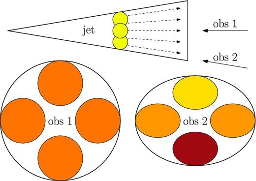
Effects of the viewing angle θobs on the relative Doppler boost (darker colour – higher Doppler factor |$\mathcal {D}$|) of local emitting regions in a conically expanding relativistic jet. Observer 1 is located at θobs ≪ θj, and observes similar Doppler factors from emitting regions located at different azimuthal angles. Observer 2 is located at θobs ∼ θj ( ∼ Γ− 1j) and observes different Doppler factors, and radiation from a more strongly boosted emitting region is observed earlier because of shorter light travel time. I propose that Observer 1 corresponds to us watching 3C 454.3, and Observer 2 corresponds to us watching other blazars producing the sample of bright flares.
Variability of bright Fermi/LAT blazars during the first year of the Fermi mission was studied comprehensively by (Abdo et al. 2010c). In particular, they studied individual flares of 10 sources of high variability index. They used light curves integrated using 3-d bins and fitted them with double-exponential flare templates allowing for arbitrary time asymmetry. They found that the average flare duration was 〈T〉 ≃ 12 d and the average flare asymmetry 〈k〉 ≃ 0.08, with broad distributions of these parameters. While both parameters were calculated in a different way than in this work, the flares studied by (Abdo et al. 2010c) are different events than the flares studied here. By using time bins of 3 d and looking at entire light curves, they picked many long gently varying components. In this work, I use 0.5-d time bins and look only at pieces of the light curves that belong to individual flares according to my definition, and I find no flares longer than 10 d. While (Abdo et al. 2010c) conclude that no particular type of flare asymmetry (positive/negative) is being favoured by their results, I show that only flares shorter than ∼1.5 d tend to be asymmetric.
4.2 Spectral properties
Average gamma-ray spectral index of the brightest blazar flares ranges between 1.9 and 2.6. As all of the studied blazars belong to the subclass of flat-spectrum radio quasars (FSRQs), these values are rather typical (Ackermann et al. 2011). I note that for the longest flares spectral indices converge into a narrow range between 2.3 and 2.4. This is most likely a statistical effect, as the average is calculated from a larger number of data points. Long flares show complex, chaotic structures in the gamma-ray flux – photon index space, and the scatter of photon index values is of the order of ±0.1. But even short flares, while they usually have simple light curves, often show a substantial photon index scatter. Individual blazars show significant differences in the spectral behaviour. PKS 1222+216 typically shows relatively hard spectra with small photon index scatter, while 3C 273 shows relatively soft spectra with high photon index scatter. Overall, the gamma-ray spectral variability of flaring blazars is completely irregular. Because of the lack of consistent patterns (e.g. CW or CCW loops), the flux – photon index diagrams are not very useful as probes of the physics of particle acceleration in FSRQs.
5 CONCLUSIONS
I selected a sample of the 40 brightest gamma-ray flares of blazars that occurred during the first four years of the Fermi mission. A flare is defined as a period of time over which the flux exceeds half of the peak value. For each flare, I calculate its peak flux, peak luminosity, duration, time asymmetry, average photon index and the photon index scatter. I present light curves and flux–photon index diagrams, and study the distributions of the flare parameters.
The sample is hosted by five blazars, of which the most active were 3C 454.3 (16 flares) and PKS 1510−089 (14 flares). In general, flares produced by 3C 454.3 are longer and more complex than those produced by other sources. This can be attributed to a very small viewing angle of 3C 454.3 (θobs ≪ θj), a consequence of which is that a larger fraction of the jet volume is strongly Doppler boosted. Other blazars, having θobs ∼ θj, produce shorter flares that are time asymmetric, with the flare onset shorter than the flare decay. This is because jet regions that are more Doppler boosted are located closer to the observer, and thus brighter subflares precede fainter ones. Long multiply peaked flares indicate fragmentation of the gamma-ray emitting regions in blazar jets. I am unable to identify any regularities in the spectral variations of flaring blazars.
I thank Aneta Siemiginowska, Mitch Begelman, Greg Madejski and Benoît Cerutti for discussions, and the anonymous reviewer for helpful comments. This work was partly supported by the NSF grant AST-0907872, the NASA ATP grant NNX09AG02G, the NASA Fermi GI programme and the Polish NCN grant DEC-2011/01/B/ST9/04845.
(Pushkarev et al. 2009) estimated the jet opening angles for the MOJAVE blazars. Their results indicate that Γjθj ≪ 1, which would not allow for high contrasts in the Doppler factors. However, this measurement, made at the frequency of 15 GHz, probes jet regions located significantly beyond the gamma-ray emission sites, as indicated by a systematic delay of the 15 GHz radio signals with respect to the gamma-rays (Pushkarev, Kovalev & Lister 2010).
