


Abstract
There are many pertinent open issues in the area of star and planet formation. Large statistical samples of young stars across star-forming regions are needed to trigger a breakthrough in our understanding, but most optical studies are based on a wide variety of spectrographs and analysis methods, which introduces large biases.
Here we show how graphical Bayesian networks can be employed to construct a hierarchical probabilistic model which allows pre-main-sequence ages, masses, accretion rates and extinctions to be estimated using two widely available photometric survey data bases (Isaac Newton Telescope Photometric Hα Survey r′/Hα/i′ and Two Micron All Sky Survey J-band magnitudes). Because our approach does not rely on spectroscopy, it can easily be applied to ho‐mogeneously study the large number of clusters for which Gaia will yield membership lists.
We explain how the analysis is carried out using the Markov chain Monte Carlo method and provide python source code. We then demonstrate its use on 587 known low-mass members of the star-forming region NGC 2264 (Cone Nebula), arriving at a median age of 3.0 Myr, an accretion fraction of 20 ± 2 per cent and a median accretion rate of 10−8.4 M⊙ yr−1.
The Bayesian analysis formulated in this work delivers results which are in agreement with spectroscopic studies already in the literature, but achieves this with great efficiency by depending only on photometry. It is a significant step forward from previous photometric studies because the probabilistic approach ensures that nuisance parameters, such as extinction and distance, are fully included in the analysis with a clear picture on any degeneracies.
1 INTRODUCTION
Large uncertainties remain with respect to the mechanisms and time-scales of star and planet formation. While it has been established that young solar-like stars stop accreting and lose their protoplanetary discs on a time-scale of ∼1–10 Myr (Haisch, Lada & Lada 2001; Fedele et al. 2010), there is no full understanding of the interplay between the various physical mechanisms which affect disc evolution (Williams & Cieza 2011).
Large statistical samples of young stars are needed to make the breakthrough in our understanding. Whilst such samples have recently become available through infrared photometry which traces circumstellar dust (Evans et al. 2009), they are not available for emission-line studies which trace material in the gas phase. Understanding the evolution of the gas with respect to the dust is of critical importance for testing competing models of disc evolution and planet formation (e.g. Najita, Strom & Muzerolle 2007; Owen, Ercolano & Clarke 2011; Espaillat et al. 2012).
Existing gas emission-line studies have mostly relied on spectroscopy, which could only be obtained for limited numbers of stars in nearby star-forming regions (e.g. Gullbring et al. 1998; Natta et al. 2004; Herczeg & Hillenbrand 2008). Moreover, it is often hard to intercompare the results from different regions because they have been obtained using a variety of spectrographs and analysis methods which complicate the analysis.
The increasing availability of data from large photometric surveys allows samples to be obtained across star-forming regions which are both larger and more homogeneous. For example, the Isaac Newton Telescope (INT) Photometric Hα Survey (IPHAS) covers 1800 deg2 of the Northern Galactic Plane using r′/i′ broad-band and Hα narrow-band filters (Drew et al. 2005; González-Solares et al. 2008). This survey is particularly relevant to star formation studies because Hα photometry allows a statistical appraisal of gas accretion rates to be made for massive clusters at large distances (De Marchi, Panagia & Romaniello 2010; Spezzi et al. 2012).
So far, we have used the IPHAS survey to study pre-main-sequence stars in just one star-forming region: IC 1396 in Barentsen et al. (2011a, hereafter Paper I). We used Hα narrow-band photometry to identify T Tauri stars and estimate their accretion rates, whilst simultaneously estimating ages and masses from the (r′ − i′)/r′ colour–magnitude plane.
Before we can apply our methodology to the entire IPHAS [and future VST Photometric H-Alpha Survey of the Southern Galactic Plane (VPHAS)] Galactic Plane region, we first need to develop more powerful tools. Whilst the results of Paper I were in good agreement with independent spectroscopic measurements, the method suffered from the drawback that a fixed amount of extinction was assumed for all objects, as there is no straightforward method to obtain this parameter simultaneously with ages, masses and accretion rates from colour–magnitude or colour–colour diagrams. The increasing sophistication of models and the so-called ‘data deluge’ from surveys requires more powerful inference tools to be adopted, as there are limitations to the information content to be extracted from 2D diagrams.
The generic mathematical solution to the problem of understanding which parameter-space regions match a set of observations is called Bayesian inference. The theoretical principles of the method have been understood for decades, but the widespread adoption in astrophysics has only taken off in recent years owing to the advances in both algorithms and computing power. So far, the Bayesian framework has become the favoured tool for e.g. the determination of cosmological parameters (Trotta 2008), the analysis of transit light curves (Ford 2005; Kipping et al. 2012) or the determination of meteor rates (Barentsen, Arlt & Frohlich 2011b). The approach has also been explored for estimating ages and extinctions for main-sequence stars (Pont & Eyer 2004; Jørgensen & Lindegren 2005; Bailer-Jones 2011). In the context of star formation, the method has recently been used to perform a dynamical membership analysis of the Sco OB2 association (Rizzuto, Ireland & Robertson 2011) and to assess the accuracy of pre-main-sequence models (Gennaro, Prada Moroni & Tognelli 2012). However, the method has so far not been used to tackle the common problem of estimating the basic parameters of individual pre-main-sequence stars.
In this paper, we show how Bayesian inference can be used to simultaneously determine extinction, stellar ages and masses and accretion rates for known members of a star-forming region. We will demonstrate the method on NGC 2264, which is one of the best-studied regions within the IPHAS survey area and has a very complete membership list (Dahm 2008; Sung et al. 2008). We note that the future Gaia astrometric survey is expected to yield accurate membership lists for hundreds of clusters (Bailer-Jones 2009), therefore our strategy to re-analyse a large sample of known cluster members in a homogeneous way is likely to become an increasingly important tool.
In Section 2 we motivate our approach and specify the model. In Section 3 we explain the application to NGC 2264, and in Section 4 we present the results. In Sections 5–7, we discuss the outcome, present future extensions and summarize the conclusions.
2 METHOD: BAYESIAN INFERENCE
Our aim is to determine ages, masses and accretion rates from IPHAS r′/i′/Hα magnitudes, while simultaneously constraining the extinction by adding Two Micron All Sky Survey (2MASS) J-band magnitudes to the data set. We employ Bayesian inference for this purpose. In Section 2.1 we describe the motivation for the method, in Sections 2.2 and 2.3 we explain the formalisms and implementation, while in Sections 2.4 and 2.5 we explain the practical use.
2.1 Motivation
2.1.1 Characteristics of T Tauri stars
In the current picture of star formation, solar-like stars are thought to assemble the majority of their mass during the first few 105 years after the initial collapse of their parent molecular cloud (Evans et al. 2009). Within ∼1 Myr the envelope of gas and dust clears and the newly formed stars become visible at optical wavelengths, from which point they are commonly called T Tauri stars. These objects continue to grow by accreting material from a circumstellar accretion disc, which does not exceed 10–20 per cent of the stellar mass and is dispersed within a few million years (Haisch et al. 2001; Hartmann 2008; Fedele et al. 2010).
Mass accretion is thought to take place along magnetic field lines which connect the disc to the star. Infalling gas is essentially on a ballistic trajectory, falling on to the stellar surface at near free-fall velocities, thereby producing hot impact shocks which generate excess ultraviolet (UV) and optical continuum emission (Calvet & Gullbring 1998; Gullbring et al. 2000). The accretion energy released in these shocks also heats the infalling gas, which in turn produces strong Hα emission.
This is illustrated in Fig. 1, where we show the literature spectra of four T Tauri stars of a similar spectral type (late K), shown in order of accretion rates which have been estimated from the UV/optical continuum excess emission. The spectra illustrate that the Hα line strength is correlated with the blue excess, both thought to be a result of the release of accretion energy. In contrast, the r′ and i′ bands appear least affected by accretion and are thus the most appropriate tracers for stellar age and mass. Hence, in our past study of IC 1396 (Paper I) we used the (r′ − i′)/r′ plane to estimate ages and masses from model isochrones, whilst using the (r′ − i′)/(r′ − Hα) plane to estimate Hα equivalent widths (EWs) and accretion rates.
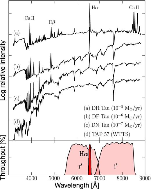
Top panel: spectra of four T Tauri stars of similar spectral type (late K) as published by Bertout (1989) shown in order of decreasing accretion rates as determined by Hartigan, Edwards & Ghandour (1995). The most notable features are (i) blue continuum excess and line veiling below ∼6000 Å; (ii) hydrogen Balmer lines in emission; (iii) Ca iiH/K and Infrared Triplet (IRT) lines in emission. The bottom spectrum is a weak-lined T Tauri star (WTTS) which does not show signs of ongoing mass accretion. Bottom panel: filter transmission curves for the IPHAS r′/Hα/i′ filters. The 2MASS J-band filter is located beyond the range of the spectra near 12 000 Å.
We note that at exceptionally high accretion rates (≳10−6 M⊙ yr−1) there is evidence for accretion-induced continuum veiling to occur in the r′ and i′ bands, which may affect the age and mass estimates. The source of the excess emission at these wavelengths is not well understood at present (Fischer et al. 2011). The effect is small and will be ignored in what follows because our study includes only objects with lower accretion rates. We will return to this topic at the end of the paper however (Section 5.3).
2.1.2 Solving the degeneracy between age, mass, extinction and Hα emission
The results obtained in Paper I were in good agreement with spectroscopic measurements from the literature. However, the method suffered from the drawback that a fixed amount of extinction was assumed for all objects because optical colour–colour diagrams show a well-known degeneracy between reddened high-mass (early-type) stars and unreddened low-mass (late-type) stars. This may surprise some readers because the (r′ − i′)/(r′ − Hα) plane is known for being able to break this degeneracy due to the strong difference in the Hα line strength between early- and late-type stars (Drew et al. 2008). However, this property cannot be exploited when Hα is in emission.
The degeneracy is illustrated in Fig. 2, where we plot the colour simulations from Paper I to show the intrinsic position of the main sequence as a function of reddening (thick and thin solid lines). These solid curves do not overlap or intersect, i.e. there is a handle on the degeneracy. However, when increasing levels of Hα emission are added (dashed lines), reddened early-type stars with Hα in emission become entangled with unreddened late-type stars.
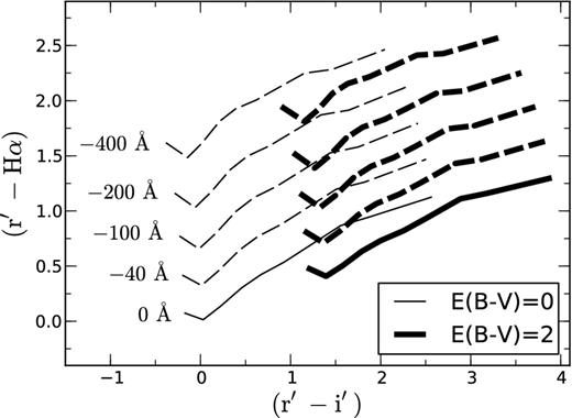
Position of the unreddened and reddened main sequence (thin and thick lines) in the IPHAS (r′ − i′)/(r′ − Hα) plane, shown from early O to late M-type stars. We also mark the position of the main sequence for increasing levels of Hα emission (dashed lines, indicated by their Hα EWs in units of Å). The figure illustrates the degeneracy between reddening, spectral type and Hα emission in this plane. These simulations are taken from Paper I.
To resolve this degeneracy, we require additional colour(s) to be added to the IPHAS data set. Our best-available option is to add the near-infrared J-band magnitude from the 2MASS survey (Skrutskie et al. 2006) because the (r′ − i′)/(i′ − J) plane can be shown to break the degeneracy between reddening and spectral type for K- and M-type objects, which constitute the vast majority of T Tauri stars (Martin 1997). At the same time, the J band is not commonly affected by excess emission from a circumstellar disc, unlike the 2MASS H and K bands at longer wavelengths (Meyer, Calvet & Hillenbrand 1997).
However, adding the J-band magnitude to our sample does not allow us to simply read the extinction for every object from the (r′ − i′)/(i′ − J) diagram straight away, as these colours do not depend on mass and extinction alone. For example, the Hα line falls inside the r′ band, such that objects with Hα in emission show an r′-band excess ranging between −0.05 mag (EWHα≅ −50 Å) and −1.0 mag (EWHα≅ −1000 Å), albeit depending on the spectral type (Paper I). In addition, the colours also depend on the stellar age as pre-main-sequence stars tend to rise in effective temperature as they approach the main sequence.
Whilst adding the J-band data should offer us sufficient information to constrain the four parameters of interest, the problem remains how these constraints can be inferred in practice?
2.1.3 Inferring parameters from photometry
The traditional method used to estimate stellar parameters from photometry is to place the observed objects in 2D colour–magnitude diagrams, together with the output of evolutionary models. Such an approach is useful when the number of free parameters is small. However, when the number of dimensions in the parameter or observable space increases, there is no obvious way to decide which plane/parameter combinations should be employed. For example, our r′/Hα/i′/J data set can be used to construct no less than 15 different colour–colour diagrams and 24 colour–magnitude diagrams, all of which depend to some extent on all of our parameters of interest.
We could devise an ad hoc algorithm to make use of all the available information, for example: we could iteratively fit model parameters in multiple planes until a certain convergence criterion is met. We can also employ a range of data modelling methods to help us link observations to parameters (e.g. Neural Networks, Principal Component Analysis). However, it is unclear how the results obtained by such methods depend on ad hoc choices made in the design of the algorithms (e.g. the structure of the Neural Network). Moreover, there is no clear way for these methods to obtain meaningful error bars which take full account of all known sources of uncertainty (Ford 2005).
A better approach is to obtain maximum likelihood estimates using expectation-maximization (EM) algorithms. These methods require the user to define a predictive model which estimates the likelihood of an observation given a set of model parameters. The model is then optimized to find the set of parameters which are most likely to explain the observed data (in the special case of a Gaussian likelihood model this is χ2fitting).
While EM presents a significant improvement over ad hoc methods, it suffers from the drawback that only a single ‘best-fitting’ point estimate is provided, regardless of whether or not a unique solution exists. This is a particular concern in astronomy, where model uncertainties and data sparsity imply that there is often a ‘family’ of likely solutions which occupy degenerate or multi-modal regions in the parameter space. This problem is often solved by keeping one or more of the degenerate ‘nuisance’ parameters fixed, but such assumptions invariably reduce the ability of the model to capture reality.
Rather than focusing on finding a ‘best-fitting’ estimate, it is better to employ the predictive model to infer the full probability distribution for all possible solutions. This approach is called Bayesian inference (though we note that some authors prefer the term probabilistic inference to distinguish the approach from best-fitting EM methods which also employ the Bayes’ theorem).
Obtaining the full distribution may seem impractical at first sight because point estimates are useful for plotting and tabulation. However, a full distribution can be reduced to a point estimate by computing the expectation value or median, which, unlike the maximum likelihood, take full account of the distribution (i.e. an expectation value minimizes the variance, while the median minimizes the mean absolute error). Moreover, knowledge of the full distribution allows meaningful confidence intervals and covariances to be quantified and visualized, by marginalizing over the nuisance parameters.
In what follows, we provide a formal description of the method and explain how it is applied to our problem.
2.2 Solution: Bayesian inference
2.2.1 Formalism
The basic idea is to create a parametrized model which is able to reproduce the data and its uncertainty, and then compare that model for different sets of parameters against the observations in a probabilistic way.
Let |$\boldsymbol {\theta }= \lbrace \theta _1,\ldots , \theta _n\rbrace$| represent a set of unknown model parameters and let |$\boldsymbol {d}= \lbrace d_1,\ldots , d_i\rbrace$| represent a set of observed data. We can construct a likelihood model|$P(\boldsymbol {d}| \boldsymbol {\theta })$| which computes the probability for an observation to occur under a given a set of parameters. Such a model can be computed using the best-available knowledge, and is limited only by scientific complexity and computing power.
2.2.2 Constructing the joint distribution
|$P(\boldsymbol {\theta }, \boldsymbol {d})$| can be thought of as the model which defines how the theoretical parameters and observations relate to each other. We now explain how this model is formulated for our application.
Notation.
| M☆ | Stellar mass (M⊙) |
| τ | Stellar age (Myr) |
| |$\dot{M}_{\rm acc}$| | Accretion rate (M⊙ yr−1) |
| Rin | Inner disc truncation radius (R☆) |
| SEDint | Modelled intrinsic SED |$\lbrace M_{{r^{\prime }}},\ M_{{H\alpha }},\ M_{{i^{\prime }}},\ M_{J} \rbrace$| |
| LHα | Excess Hα luminosity (L⊙) |
| EWHα | Hα emission equivalent width (Å) |
| d | Distance (pc) |
| A0 | Extinction parameter (mag) |
| SEDapp | Modelled apparent SED |$\lbrace m_{{r^{\prime }}},\ m_{{H\alpha }},\ m_{{i^{\prime }}},\ m_{J} \rbrace$| |
| SEDobs | Observed SED |$\lbrace {r^{\prime }},\ {H\alpha },\ {i^{\prime }},\ J,\ {\sigma _{r^{\prime }}},\ {\sigma _{\rm H\alpha }},\ {\sigma _{i^{\prime }}},\ \sigma _{J}\rbrace$| |
Having defined θ and d, we now formulate |$P(\boldsymbol {\theta },\boldsymbol {d})$|. This is a complex distribution with a high number of dimensions. It would be tedious to construct a single function which computes its value for all possible combinations of θ and d. We can greatly reduce the complexity however by exploiting the fact that many of the variables can be assumed to have (conditional) independence relationships.
A convenient and concise way to represent the dependencies amongst variables is to use a directed acyclic graph (i.e. a graph with no loops), often referred to as a probabilistic graphical model or a Bayesian network. These terms are synonyms for a syntactic method whereby variables are represented by nodes in a graph, and dependencies between those variables are represented by arrows. Intuitively, an arrow from variable A to B indicates that A has a direct influence on B. Formally, the Bayesian network is constructed as follows (Russell & Norvig 2009):
Each node corresponds to a variable from θ or d.
A set of arrows connect pairs of nodes. If there is an arrow from node A to node B, then A is said to be a parent of B. Pairs of nodes which are not directly connected by an arrow represent variables which are assumed to be conditionally independent of each other given their parents.
The graph should not have directed cycles, this would be a sign of recursive reasoning.
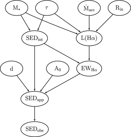
Bayesian network representing the dependencies between the variables in our inference model. Nodes which are not directly connected represent variables which are conditionally independent of each other given their parents.
2.3 Priors and likelihoods
2.3.1 Priors
A challenge that comes with the use of Bayes’ theorem is the choice of the priors. We should not shy away from this task however, as there is no inference without assumptions. Being forced to define them in a clear way can be seen as an advantage over other methods (e.g. χ2 fitting bears the implicit assumption of uniform priors on the free parameters, yet the consequence of this assumption is rarely considered). In the case of our most influential prior, P(A0), we will quantify the extent of its influence in Section 5.4.
The prior distributions are summarized in Table 2 and explained as follows.
Summary of priors. |$\mathcal {U}({\rm min,max})$| denotes a uniform distribution, while |$\mathcal {N}(\mu ,\sigma )$| denotes a Gaussian.
| Prior | Distribution |
|---|---|
| P(M☆) | $\sim \left\lbrace \begin{array}{ll}{M_{\ast}}^{-1.3}\,\hphantom{2.3} \qquad{if\ \ } 0.1 < {M_{\ast}}< 0.5 \\
0.5\,{M_{\ast}}^{-2.3} \qquad {if\ \ } 0.5 \le {M_{\ast}}< 7 \end{array} \right.$ |
| P(log τ) | |$\sim \mathcal {U}(5, 8)$| |
| P(log |$\dot{M}_{\rm acc}$|) | |$\sim \mathcal {U}(-15, -2)$| |
| P(Rin) | |$\sim \mathcal {N}(5, \sigma =2) ({R_{\rm in}}> 1)$| |
| P(d) | |$\sim \mathcal {N}(760, \sigma =5)$| |
| P(log A0) | |$\sim \mathcal {N}(-0.27, \sigma =0.46)$| |
P(M☆): the mass prior follows the initial mass function (IMF) due to Kroupa (2001), truncated between 0.1 and 7 M⊙ which are the limits of the stellar evolutionary model that we adopt in what follows. Objects outside this range are either saturated or fall below the detection limit of the IPHAS survey and so these truncation limits do not affect our results, other than constraining the parameter space to a sensible domain.
P(τ): the age prior is assumed uniform in the logarithm and truncated between 0.1 and 100 Myr, which again corresponds to the limits of the evolutionary model.
P(|$\dot{M}_{\rm acc}$|): the accretion rate prior is assumed uniform in the logarithm and is truncated between 10−15 and 10−2 M⊙ yr−1. This range entails all the accretion rates commonly reported in the literature and goes well below the typical detection limit of ∼10−10 M⊙ yr−1 we found in Paper I.
P(Rin): the disc truncation radius follows a Gaussian distribution with a mean of 5 R☆ and standard deviation 2 R☆. This is a commonly used assumption based on the typical co-rotation radius of T Tauri stars (Gullbring et al. 1998).
P(d): for the distance prior we adopt a Gaussian distribution centred on the widely cited distance towards NGC 2264 of 760 pc (Sung, Bessell & Lee 1997). The standard deviation of 5 pc reflects the approximate diameter of the cluster and therefore the uncertainty in our results will reflect only the relative distance errors. We note that a recent distance estimate by Baxter et al. (2009) puts the region at 913 pc and so the systematic error in the distance may be significantly larger than 5 pc. However, because we aim to investigate the relative properties of objects in the cluster, rather than systematic errors for the cluster as a whole, we opt not to model the absolute distance uncertainty here. (Note that the Gaia survey will remove most of this uncertainty in the future.)
P(A0): for the extinction parameter we adopt the empirical distribution of extinction for 202 candidate members as determined by Rebull et al. (2002) on the basis of moderate-resolution spectroscopy of low-mass objects in NGC 2264. We found that their distribution can be well approximated as a log-normal with mean log A0 = −0.27 (A0 = 0.54) and a broad standard deviation σlog A0 = 0.46.
2.3.2 SEDint likelihood (equation 14)
The intrinsic SED of a young star is predicted as a function of mass and age as follows.
First, intrinsic broad-band magnitudes |${M_{r^{\prime }}}$|, |${M_{i^{\prime }}}$| and MJ are interpolated from the evolutionary model due to Siess, Dufour & Forestini (2000) for solar metallicity (Z = 0.02). Their model consists of 29 separate mass tracks from 0.1 to 7 M⊙ from which isochrones can be computed using an online tool.1 We used this tool to download the model at 50 different ages ranging between 0.1 and 100 Myr, i.e. we obtained a dense sampling of the model in 1450 discrete points as a function of mass and age (=29 × 50 points).
The Siess et al. model provides intrinsic magnitudes on the basis of the empirical conversion tables presented by Kenyon & Hartmann (1995), which provide intrinsic colours and bolometric corrections as a function of stellar effective temperature. These tables only provide a calibration for the Cousins photometric system however, so we had to convert the model RC/IC magnitudes to IPHAS r′/i′ using the transformations given in Paper I.
We then approximated the evolutionary model as a continuous function by fitting 1450 radial basis functions (RBF) to the collection of discrete model points using the python module http://scipy.interpolate.rbf (cf. Appendix A). The resulting set of basis functions provides us with an accurate and fast tool to interpolate values from the grid.
Having obtained intrinsic magnitudes as a function of age and mass, we then predict the narrow-band magnitude MHα using the grid of IPHAS colour simulations presented in Paper I, where we determined the intrinsic colour (r′ − Hα) as a function of (r′ − i′) on the basis of a library of observed spectra.
2.3.3 LHα likelihood (equation 15)
Hα is the strongest emission line due to accretion, and its intensity can be used to trace the accretion luminosity.
As explained in Section 2, accretion is thought to take place along magnetic field lines which act as channels connecting the disc to the star from an inner disc truncation radius Rin. The infalling gas is essentially on a ballistic trajectory, falling on to the star at near free-fall velocities, producing a hot impact shock (Calvet & Gullbring 1998; Gullbring et al. 2000). The energy released in these shocks heats the infalling circumstellar gas, which explains the Hα emission.
2.3.4 EWHα likelihood (equation 16)
The uncertainty associated with the conversion of LHα into EWHα can be assumed negligible and for simplicity we take the likelihood to be deterministic.
2.3.5 SEDapp likelihood (equation 17)
The apparent SED is obtained by correcting the intrinsic SED for the effects of distance, extinction and Hα emission in three steps.
First, the distance modulus 5 log (d) − 5 is added to each of the intrinsic magnitudes. Secondly, offsets for the r′/Hα/i′ magnitudes are obtained as a function of A0 and EWHα by means of RBF interpolation from the pre-computed grid of simulated photometry from Paper I. Finally, the offset for the J magnitude for extinction is computed using the reddening law due to Schlegel, Finkbeiner & Davis (1998). The J-band offset cannot be computed in the same way as the other bands because the optical spectral library on which our grid of simulated colours is based does not extend far enough into the near-infrared.
Again, this likelihood is assumed deterministic.
2.3.6 SEDobs likelihood (equation 18)
We found empirically that a value of σcal = 0.1 is required to prevent the expected match between the observed data and the modelled SED to be too exact. Leaving this term out has the effect of producing a complex multi-modal probability landscape which prevents the sampling algorithm – discussed below – from converging efficiently. The term can be considered as a way to account for all those sources of noise which we could not explicitly model in the other parts of the model.
2.4 Sampling the joint distribution using MCMC
In the previous sections, we defined the joint distribution |$P(\boldsymbol {\theta }, \boldsymbol {d})$| and thus the posterior |$P(\boldsymbol {\theta }| \boldsymbol {d})$| as a product of priors and likelihoods. At this point, the question remains how this distribution is computed in practice. A simple ‘brute force’ method which computes the model for the entire parameter space is computationally intractable. Even if we were to sample the parameter space at a coarse resolution, say, 100 values for each of the 10 model parameters, we would require the distribution to be computed in 1020 points. This would occupy the author's computer for many billion years.
Fortunately, probability distributions can be sampled efficiently using a specialized class of algorithms called Markov chain Monte Carlo (MCMC). In brief, MCMC algorithms generate a pseudo-random walk in the parameter space in such a way that, over time, points in the space are visited with a frequency that is proportional to a specified probability distribution. Only useful points in the parameter space tend to be evaluated and we avoid wasting time calculating an infinite number of points in the improbable regions. The details of MCMC algorithms are beyond the scope of this paper but we recommend Chib & Greenberg (1995) for an introduction and MacKay (2003) and Gregory (2005) for background reading.
Several libraries are available which allow Bayesian models to be defined and sampled using MCMC. In this work, we used the pymc framework for python (Patil, Huard & Fonnesbeck 2010) which has the advantage that it allows models to be defined in a very concise way. Our annotated model takes less than two pages and is therefore included at the end of this paper for easy reference (Appendix A). As such, this paper contains a precise and repeatable specification of the parameter estimation procedure. The source code and accompanying files are also available from the GitHub repository of the author.2
For each object under study in this paper (to be explained in Section 3), we sampled the joint distribution using the default settings of pymc, which is to use the traditional Metropolis–Hastings walking algorithm with a Gaussian step proposal function (we refer to the manual of pymc for definitions of these technical terms). pymc automatically tunes the size of the step proposal function to ensure the walk is made efficiently with an acceptance rate between 20 and 50 per cent.
It is usually sufficient to sample a probability distribution in only a few hundred independent points to obtain a sufficiently accurate approximation. MCMC algorithms typically require far more samples to be obtained however because the walking algorithm naturally produces chains which are auto-correlated and hence may be stuck at local maxima. The true number of iterations which are required depends on the shape of the probability landscape; a complex or multi-modal distribution with sharp hills and valleys tends to require far more samples. In our application we find the chains to be auto-correlated over a typical length of 50–250 steps (depending on the properties of the star). For this reason, we decided to sample each object in 250 000 points such that the total number of points is at least three orders of magnitude larger than the auto-correlation effect (i.e. at least 1000 truly independent samples are obtained for each object).
It is likely that our application would profit from recent advances in MCMC algorithms which claim to reduce the auto-correlation effect considerably. We draw the reader's attention to an implementation of such algorithm made available by Foreman-Mackey et al. (2012) which we intend to evaluate in future work.
2.5 Results of the sampling procedure
To verify the reliability of our procedure, the sampling was carried out using five independent walks of 50 000 steps, each starting at randomized positions (with a burn-in length of 1000 steps). We consistently found these independent chains to converge to the same parameter-space regions of high likelihood within a few hundred iterations, i.e. fast convergence towards a global maximum was reached in all cases.
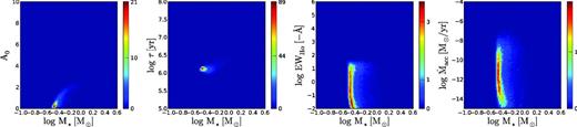
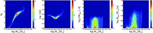
We visualized the samplings by means of 2D histograms (Figs 4–7), which trace the posterior marginalized over all other parameters. The first two examples (Figs 4 and 5) are representative for the vast majority of objects in our study which show low levels of extinction (A0 < 1). The main difference is that the first example shows evidence for Hα emission, whereas the second example does not.
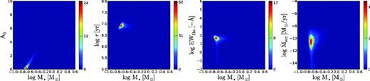
Normalized 2D histograms of the distribution of points in the MCMC for object C11059 (r′ = 19.4 ± 0.03; r′ − Hα = 1.3 ± 0.04; r′ − i′ = 1.9 ± 0.04; i′ − J = 2.1 ± 0.06). These histograms trace the posterior distributions marginalized over all other parameters. Blue regions show areas in the parameter space with low probability, red areas show areas with high probability.
Histograms for object C15152 (r′ = 16.3 ± 0.002; r′ − Hα = 0.8 ± 0.004; r′ − i′ = 1.4 ± 0.003; i′ − J = 1.7 ± 0.02). Compared to the first example, this is a brighter object with near-zero Hα emission and a slightly higher mass. The probability region is marginally more condensed owing to the smaller photometric uncertainties.
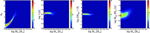
Histograms for object C29493 (r′ = 19.3 ± 0.04; r′ − Hα = 0.7 ± 0.08; r′ − i′ = 2.0 ± 0.05; i′ − J = 3.1 ± 0.04). Compared to the first example shown in Fig. 4, the i′ − J colour is significantly redder which results in a higher extinction. We also draw attention to the banana-like shape of the high-probability region, which is a result of changes in the direction of the model isochrones relative to the reddening vector.
Histograms for object C36902 (r′ = 20.6 ± 0.09; r′ − Hα = 1.6 ± 0.11; r′ − i′ = 2.1 ± 0.10; i′ − J = 3.1 ± 0.07). This is one of the lowest mass objects in our study. The high-probability region appears to go slightly beyond the range of the Siess et al. model.
Non-typical examples are shown in Figs 6 and 7. These objects have (i′ − J) colours which are significantly redder compared to the first two examples, in a way that is consistent with a higher level of extinction. We note that the uncertainties are significantly larger for these more highly reddened objects. This is a result of our decision to adopt a log-normal extinction prior with a peak near A0 = 0.5 and a long tail towards higher values (corresponding to the empirical distribution for the region which we adopted in Section 2.3).
If we had not included this prior information then the uncertainty in Figs 4 and 5 would have been similar to that in Figs 6 and 7. In other words, whilst our data set offers a rough constraint on the individual extinction, the degeneracy between extinction and mass is not resolved entirely and the prior makes a contribution towards constraining the result. At the same time, Figs 6 and 7 demonstrate that the prior does not prevent higher levels of extinction and uncertainty to be revealed when the data are inconsistent with low extinction. We will quantify the contribution of the prior in the discussion at the end of the paper (Section 5.4).
We draw the reader's attention to the ‘banana’-shaped posterior which appears when the uncertainty is large. This is a natural result of curves in the model evolutionary tracks relative to the reddening vector.
We also note that the range of possible masses in Fig. 7 appears to go somewhat beyond the mass range that is provided by the Siess et al. model. Only a few faint objects are affected in this way however, and we decided not to remove these from our study.
Finally, we note that a visual inspection of all objects under study revealed that these marginalized posteriors distributions are single-moded and quasi-symmetric when the logarithm of each parameter is considered. This implies that the marginalized posterior can be well characterized by means of computing expectation values and standard deviations.
The posterior was sampled and characterized in this way for a total of 587 known members of the NGC 2264 star-forming region. In the following sections, we discuss how the input data set was obtained (Section 3) and how the derived parameters make sense of the objects’ positions in colour–magnitude diagrams (Sections 4 and 5).
3 APPLICATION TO NGC 2264
NGC 2264, also known as the Cone Nebula or Christmas Tree Cluster, is located at a distance of ∼760 pc in the constellation of Monoceros (Sung et al. 1997). The cluster is estimated to contain ∼1000 members, most of which have been identified using a range of methods including Hα and variability surveys, X-ray observations and mid-infrared imaging (a review is given by Dahm 2008).
Stellar parameters have previously been estimated for members of the region using a wide variety of colour–magnitude diagrams and evolutionary models (e.g. Park et al. 2000; Rebull et al. 2002; Sung, Bessell & Chun 2004; Flaccomio, Micela & Sciortino 2006; Dahm et al. 2007). There are significant systematic differences between these studies however, with median age estimates for the cluster ranging between ∼1 and 5 Myr (Dahm 2008).
Moreover, there is only a partial overlap in the membership samples considered in these previous studies, owing to differences in the data sets and member selection criteria. In what follows, we attempt to select the largest and most homogeneous membership sample of NGC 2264 to date, and then use it to demonstrate our method.
3.1 Membership list
The most comprehensive catalogue of objects towards NGC 2264 has been presented by Sung et al. (2008, hereafter S08) and Sung, Stauffer & Bessell (2009, hereafter S09). Their work is based on a compilation of the following.
Deep VRI and Hα photometry using the 3.6-m Canada–France–Hawaii Telescope (CFHT).
Bright BVRI and Hα photometry using the 1-m telescope at Siding Spring Observatory (SSO).
Low- and moderate-resolution literature spectroscopy from Reipurth et al. (2004) and Dahm & Simon (2005).
Archival X-ray observations from the Chandra and ROSAT space telescopes.
Archival infrared observations from the Spitzer Space Telescope.
The authors constructed a catalogue of 69 674 optical objects detected towards the cluster (tables 3, 8 and 9 in S08) and then assigned various ‘membership codes’ by cross-matching the Hα, X-ray and infrared data. We used these codes to select a total of 1191 likely members which satisfy one or more of the following criteria.
Hα emission stronger than chromospherically active main-sequence stars (membership code: ‘H’, ‘E’, ‘+’, ‘P’ or ‘p’).
Strong X-ray emission (code: ‘X’, ‘+’, ‘-’, ‘M’ or ‘P’).
Spitzer colours consistent with a protoplanetary disc (code: ‘I’, ‘II’, ‘II/III’, ‘pre-TD’ or ‘TD’ in S09).
IPHAS and 2MASS photometry for known members of NGC 2264 which satisfy our selection and quality criteria (see the text). Column 1 shows the existing object identifier as defined by Sung et al. (2008), while column 2 shows the IAU-registered naming convention for objects detected by the IPHAS survey, which is formed by prefixing ‘IPHAS’ to the position string. Calibrated IPHAS photometry is given in columns 3–5 and matched 2MASS data are given in columns 6–8. This table is available in its entirety in the online journal.
| Name (S08) | IPHAS ID J[RA(2000)+Dec.(2000)] | IPHAS magnitudes | 2MASS magnitudes | ||||
|---|---|---|---|---|---|---|---|
| r′ | Hα | i′ | J | H | K | ||
| C11059 | J063955.90+094239.8 | 19.41 ± 0.03 | 18.14 ± 0.03 | 17.56 ± 0.02 | 15.44 ± 0.06 | 14.69 ± 0.05 | 14.28 ± 0.08 |
| C11997 | J063957.95+094104.7 | 17.91 ± 0.01 | 16.50 ± 0.01 | 16.16 ± 0.01 | 14.36 ± 0.04 | 13.65 ± 0.03 | 13.35 ± 0.04 |
| C12135 | J063958.30+092848.6 | 18.51 ± 0.01 | 17.66 ± 0.02 | 16.74 ± 0.01 | 14.99 ± 0.04 | 14.34 ± 0.05 | 14.11 ± 0.07 |
| C12598 | J063959.23+100607.7 | 17.26 ± 0.00 | 16.18 ± 0.01 | 16.07 ± 0.00 | 13.91 ± 0.02 | 12.80 ± 0.03 | 12.10 ± 0.02 |
| C13507 | J064001.30+094300.5 | 19.10 ± 0.04 | 16.91 ± 0.01 | 18.14 ± 0.04 | 15.00 ± 0.04 | 13.17 ± 0.02 | 11.94 ± 0.03 |
| C14005 | J064002.67+093524.3 | 16.86 ± 0.00 | 15.87 ± 0.00 | 15.35 ± 0.00 | 13.70 ± 0.03 | 12.99 ± 0.03 | 12.71 ± 0.03 |
| C15152 | J064005.22+095056.6 | 16.27 ± 0.00 | 15.50 ± 0.00 | 14.87 ± 0.00 | 13.19 ± 0.02 | 12.48 ± 0.02 | 12.26 ± 0.02 |
| C15247 | J064005.53+092226.1 | 16.54 ± 0.00 | 15.65 ± 0.00 | 15.44 ± 0.00 | 13.95 ± 0.03 | 13.12 ± 0.02 | 12.73 ± 0.03 |
| C15285 | J064005.53+094554.8 | 18.54 ± 0.02 | 18.14 ± 0.04 | 17.16 ± 0.02 | 15.14 ± 0.05 | 14.28 ± 0.04 | 13.93 ± 0.05 |
| C15519 | J064006.00+094942.7 | 16.44 ± 0.00 | 15.62 ± 0.00 | 15.18 ± 0.00 | 13.46 ± 0.03 | 12.76 ± 0.03 | 12.45 ± 0.03 |
| ⋅⋅⋅ | |||||||
In this sample of 1191 objects, 42 per cent satisfy the Hα criterion, 62 per cent satisfy the X-ray criterion and 38 per cent satisfy the Spitzer criterion. There is considerable overlap: 32 per cent satisfy more than one criterion while 10 per cent satisfy all three.
Additional signatures of membership such as radial velocities, or chemical indicators of youth such as lithium, are currently not available for most of these objects. This is, in part, because half of the sample is fainter than V > 18 for which high-resolution spectroscopy becomes increasingly expensive. Based on the clustering properties and positions in the colour–magnitude diagram however, S08 convincingly argued that the vast majority of objects in this sample are genuine members of NGC 2264. Nevertheless, it is likely that our sample contains a small number of foreground/background objects.
The spatial distribution of the sample is shown in Fig. 8 together with the footprints of the observations from which the sample was compiled.
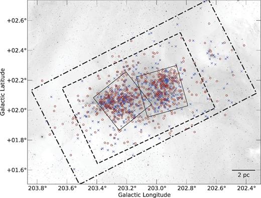
Spatial distribution of known candidate members in NGC 2264 taken from the works by Sung et al. (see the text.) Red circles show objects for which high-reliability IPHAS and 2MASS photometry is available which satisfy the strict quality requirements defined in Section 2.4; these are the objects which are studied in our work. Blue crosses show candidate members for which we could not obtain high-quality IPHAS/2MASS photometry. Large rectangles show the footprints of the deep optical CFHT observations (dash–dotted line), Spitzer IRAC observations (dashed line) and Chandra observations (solid line). A few objects fall outside these footprints because they were included on the basis of bright optical photometry or literature spectroscopy (footprints not shown). The background image is an inverted version of Fig. 9.
3.2 IPHAS counterparts
IPHAS is a 1800 deg2 photometric survey of the Northern Galactic Plane (30o ≲ ℓ ≲ 220o, −5o ≲ b ≲ +5o) carried out using a narrow-band Hα filter and the broad-band Sloan r′ and i′ filters, using the 0.3 deg2 Wide Field Camera (WFC) at the 2.5-m INT in La Palma. Data towards NGC 2264 were obtained as part of the survey during several observing runs between 2003 and 2009. The central part of the cluster, containing the vast majority of members, was observed on 2008 January 17 with an average seeing of 1.2 ± 0.1 arcsec (IPHAS field numbers 3773 and 3773o).
We used the montage toolkit to create an Hα mosaic of 20 fields towards the region which is shown in Fig. 9. The contrast of the mosaic has been stretched using an arcsinh curve to bring out the Hα background emission.
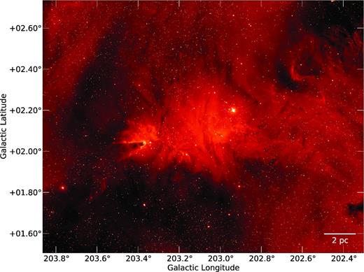
Mosaic of IPHAS observations towards NGC 2264 in the Hα band. A few narrow black bands can be seen, which indicate small gaps of missing data which will be completed in a future IPHAS data release.
All data were pipeline processed at the Cambridge Astronomical Survey Unit (CASU) as detailed in Irwin & Lewis (2001), Drew et al. (2005) and González-Solares et al. (2008). This routinely includes photometric calibration based on nightly standard star fields, with all magnitudes based on the Vega system. In addition, we have been able to draw upon the results of a global calibration of the survey data which significantly reduces field-to-field magnitude shifts (Farnhill et al., in preparation).
We cross-matched the sample of 1191 members from S08 against the IPHAS catalogue. The astrometry of both S08 and IPHAS is based on 2MASS reference coordinates which offers a typical accuracy of 0.1–0.2 arcsec (González-Solares et al. 2008). For this reason, we decided on a strict matching distance upper bound of 0.5 arcsec. total of 819 members were found to have a counterpart within the matching distance in all three IPHAS bands. For 72 of these objects, Hα photometry was not previously available in the S08 catalogue.
From the 372 objects which could not be matched in all three bands, 249 fall below the typical detection limit of IPHAS (R > 20) and 44 are saturated (R < 13). Most of the remaining objects were found to be blended with a nearby neighbour in IPHAS while being resolved in the higher resolution CFHT-based data from S08, which produces an astrometric offset. Increasing our matching distance to 1.0 arcsec would include 35 of these objects, but we decide against this in favour of data reliability.
In the majority of cases, the matched objects were detected two or three multiple times by the IPHAS survey, usually in the same night. This is because IPHAS fields are observed twice with a small offset to account for gaps between CCD chips in the camera. When two or more detections of the same object are available, we derived the mean magnitude and updated the uncertainty.
3.3 New candidate members from IPHAS
Having obtained a sample of 819 very likely members from the literature, we carried out a search in the IPHAS data base for any new Hα emitters which may have been missed during previous searches. Using the method detailed in Paper I, we identified a total of 164 objects which are located confidently above the main locus of stars in the IPHAS (r′ − i′)/(r′ − Hα) diagram. The selection threshold explained in Paper I is designed to avoid chromospherically active field stars, and so the vast majority of these objects are likely to be accreting T Tauri stars.
We find that 150 (91 per cent) of these objects were already selected because they are classified as strong Hα emitters in S08, while a further nine objects were selected on the basis of their X-ray or infrared emission but not on the basis of Hα (object IDs: C27213, C34019, C36055, C37804, C39811, C42487, C8431, W3407 and W5604). Only five objects were not already selected and are added to our sample (C18650, C19751, C25302, W2320 and W5620). This brings the sample size to 824 objects. The fact that we are unable to identify a significant number of new Hα emitters suggests that the sample is very complete in this respect, at least down to the detection limits of IPHAS.
3.4 Quality criteria
At this point, we could continue our investigation with all of the 824 objects for which IPHAS counterparts were found. However, we choose to narrow down the sample to 587 objects using the following strict quality requirements.
The photometric uncertainty on each of the three IPHAS magnitudes must be smaller than 0.1.
Each object must be classified as ‘strictly stellar’ or ‘probable stellar’ in the IPHAS catalogue in all three bands (quality flag ‘−1’ or ‘−2’ defined by González-Solares et al. 2008).
The object must have a J-band counterpart in the 2MASS data base with signal-to-noise ratio (S/N) > 5 (quality flag ‘A’, ‘B’ or ‘C’).
The object must not be marked as an unresolved binary in the catalogue due to S08 or 2MASS (flag ‘D’) and its nearest neighbour must be further away than 1 arcsec.
Criterion (i) avoids faint sources with high uncertainties. The criterion corresponds to an S/N of 10 or typical magnitude limits of 20.5 in r′ and 19.5 in i′/Hα (González-Solares et al. 2008), although we note that there are small spatial variations in the true magnitude limits depending on the observing conditions and the number of repeat observations. Only 34 objects did not meet this criterion.
Criterion (ii) deals with the issue of flux contamination. The magnitudes in the IPHAS data base are based on aperture photometry which is prone to contamination by nearby neighbours or spatially varying background emission. The IPHAS pipeline solves this problem by tracking variations in the background emission on scales of 20–30 arcsec. In some cases, the background changes on scales smaller than 5–10 arcsec; however, in which case photometric measurements of faint sources become unreliable.
Fortunately, photometry which is unreliable for this reason is flagged in the pipeline as part of the morphological classification step (see section 2.1 in Paper I). In brief, the pipeline derives a curve of growth for each object from a series of aperture flux measures with different aperture radii. When this curve deviates from the characteristic point spread function (PSF) of other stars in the field, the object is flagged as ‘extended’ (class 1) or ‘probable extended’ (class −3).
By requiring objects to be classified as ‘strictly stellar’ (code −1) or ‘probable stellar’ (code −2) in all three bands, we ensure that only reliable measurements for objects with a normal-shaped PSF are included in our analysis. A total of 143 objects did not meet this criterion.
Criterion (iii) is introduced because IPHAS magnitudes alone are not sufficient to constrain the extinction of individual objects as we explained in Section 2. A total of 62 objects did not meet this criterion. Future work could benefit from the deeper J-band data offered by the UK Infrared Deep Sky Survey (UKIDSS; Lucas et al. 2008), but data for NGC 2264 are not yet available from that survey at this time.
Finally, criterion (iv) avoids likely problems due to source confusion. A total of 30 objects did not meet this criterion.
After applying each of the criteria, we are left with 587 objects (because a number of objects failed more than one criterion). The resulting table of IPHAS and 2MASS photometry for these objects is given in Table 3 and forms the basis for our analysis.
4 RESULTS
We obtained Bayesian posterior distributions for each of the 587 objects selected above. We then summarized the posteriors by computing marginalized means and standard deviations, i.e. we derived a point estimate per parameter for each object. These values are listed in Table 4 and visualized by histograms in Fig. 10. In this section, we provide a brief overview of the results by inspecting the distributions of these point estimates. This will lead us to a set of preliminary results on the properties of NGC 2264, such as its mass distribution, median age and fraction of accretors.
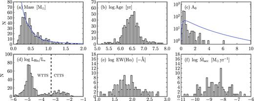
Distribution of inferred parameters listed in Table 4. Blue solid lines in panels (a) and (c) show the priors. We note that panels (e) and (f) only include the CTTS objects. We warn that these histograms do not reflect the underlying uncertainties and degeneracies.
Posterior expectation values and standard deviations for parameters of NGC 2264 members, obtained from IPHAS and 2MASS photometry using Bayesian inference. Shown here are the first 10 entries, the table is available in its entirety in the online journal.
| Name | log A0 (mag) | log M☆ (M⊙) | log τ (yr) | |$\log {EW_{\rm H\alpha }}$| (−Å) | |$\log {L_{\rm H\alpha }}$| (L⊙) | |$\log {\dot{M}_{\rm acc}}$| (M⊙ yr− 1) | Comments |
|---|---|---|---|---|---|---|---|
| C11059 | −0.41 ± 0.44 | −0.61 ± 0.08 | 6.91 ± 0.09 | 1.45 ± 0.54 | −4.5 ± 0.6 | ||
| C11997 | −0.39 ± 0.40 | −0.49 ± 0.07 | 6.50 ± 0.10 | 1.79 ± 0.16 | −3.6 ± 0.2 | −9.1 ± 0.8 | CTTS |
| C12135 | −0.33 ± 0.38 | −0.51 ± 0.07 | 6.77 ± 0.09 | −0.20 ± 0.85 | −5.8 ± 0.9 | ||
| C12598 | 0.27 ± 0.39 | −0.18 ± 0.17 | 6.56 ± 0.31 | 1.59 ± 0.86 | −3.1 ± 1.0 | −8.5 ± 1.4 | CTTS |
| C13507 | 0.19 ± 0.73 | −0.34 ± 0.28 | 6.83 ± 0.44 | 1.41 ± 2.86 | −3.8 ± 3.0 | −8.8 ± 3.3 | CTTS |
| C14005 | −0.42 ± 0.42 | −0.41 ± 0.07 | 6.28 ± 0.07 | 0.49 ± 1.13 | −4.5 ± 1.2 | ||
| C15152 | −0.33 ± 0.40 | −0.36 ± 0.09 | 6.12 ± 0.08 | −0.61 ± 1.18 | −5.3 ± 1.2 | ||
| C15247 | −0.48 ± 0.41 | −0.29 ± 0.10 | 6.59 ± 0.19 | 1.00 ± 0.98 | −3.9 ± 1.0 | ||
| C15285 | 0.21 ± 0.27 | −0.32 ± 0.14 | 7.04 ± 0.24 | −0.86 ± 0.92 | −6.2 ± 0.9 | ||
| C15519 | −0.36 ± 0.45 | −0.32 ± 0.12 | 6.27 ± 0.13 | −0.44 ± 1.44 | −5.2 ± 1.5 | ||
| ⋅⋅⋅ |
Whilst point estimates of stellar parameters are widely used as a tool to investigate the properties of a cluster, we warn that the presence of large uncertainties can make a direct analysis of point estimates unreliable. For example, while it is tempting to estimate the age of NGC 2264 from the histogram of mean stellar ages shown in Fig. 10, the result may be biased due to the presence of asymmetric and correlated uncertainties (see Pont & Eyer 2004). This does not imply that our results cannot be used to study the properties of the cluster, in fact our posteriors contain all the required information on the uncertainties and degeneracies. In order to exploit this information however, we would need to build a probabilistic model which links the global parameters of the cluster to the posteriors of the stars.
Whilst it is easy to see that our hierarchical model may be extended to include the global properties of the cluster as parameters, the priors and likelihoods of such parameters would have to be chosen with care. They would need to reflect the current knowledge in the field and allow the right questions to be answered. For example, if we were to estimate the age and age spread of the cluster, we would need to make a detailed appraisal of the accuracy of pre-main-sequence isochrones and include the information in the model.
Defining such a cluster model is beyond the scope of the present work. In what follows we merely offer the reader a concise summary of the distribution of the point estimates, which may be considered as a first-order approximation of the global properties of NGC 2264. In Section 6, we will discuss the future prospect of extending our work to obtain a complete model of the cluster.
4.1 Masses, ages and extinction
The mass distribution (Fig. 10 a) shows the expected power-law increase towards lower masses. Compared with the Kroupa IMF (blue solid line), we find a deficit of objects with masses below 0.25 M⊙. Our sample is significantly less complete below this mass due to the S/N quality criteria imposed in Section 2.4. Similarly, many stars with masses heavier than ∼1.2 M⊙ are missing due to the saturation limits of the IPHAS survey. The highest inferred mass in our sample equals 1.8+ 0.3− 0.2 M⊙.
The age distribution (Fig. 10b) shows a mean age of log τ = 6.48 ± 0.38 (which corresponds to the median τ = 3.0 Myr), albeit with a large apparent dispersion between 1.8 and 4.5 Myr (25 and 75 per cent quartiles). Our median estimate of 3 Myr is identical to the main-sequence turn-off age obtained in the seminal paper by Walker (1956), and is also consistent with the age of 3.1 Myr reported by Sung et al. (2004) using the same set of isochrones as in our work.
The extinction (Fig. 10c) shows a mean of log A0 = −0.37 ± 0.20 (A0 = 0.43) which is consistent with the widely reported low levels of foreground extinction. 30 objects show higher levels of extinction ranging between A0 = 1 and 3, while only four objects show extinctions beyond A0 > 3 (beware that the vertical axis in Fig. 10 c is logarithmic for clarity).
Compared to the log-normal extinction prior (solid blue line) there is a deficit of objects with large extinctions, which will be discussed in Section 5.4.
4.2 Hα emission and accretion rates
The Hα luminosities (Fig. 10 d) are shown as a fraction of the object's bolometric luminosity L☆ which we derived from the Siess et al. model as a function of an object's age and mass. This allows us to show the distribution relative to the chromospheric saturation limit at log LHα/L* = −3.3 (dashed line). This is the maximum level of Hα emission observed in clusters at the age of 65–125 Myr, where accretion is thought to have ceased and Hα emission is produced entirely by chromospheric activity (Barrado y Navascués & Martín 2003).
This saturation limit is a widely used criterion to separate accreting from non-accreting objects. In the remainder of this paper, we refer to objects which fall above the limit as ‘accretors’ or Classical T Tauri Stars (CTTS) while those which fall below the limit are ‘non-accretors’ or Weak-lined T Tauri Stars (WTTS).
According to this definition, the accretion fraction is 20 ± 2 per cent (115 objects). This fraction may be slightly underestimated because 36 additional objects fall only just below the criterion (log LHα/L* between −4.0 and −3.3). It is likely that some of these objects are undergoing very low levels of mass accretion which we cannot distinguish from chromospheric activity using our data set. If we were to assume that all these objects are undergoing accretion then the fraction of accreting stars would rise to 25 per cent. We note that a frequency of 20–25 per cent for a cluster of 3 Myr is in excellent agreement with other clusters of a similar age (Fedele et al. 2010).
The Hα EW distribution for the accreting stars (Fig. 10e) shows a range from −12 to −546 Å. The corresponding mass accretion rates (Fig. 10f) range from 10−10.7 to 10−6.4 M⊙ yr−1 with a median of 10−8.4 M⊙ yr−1. They are in broad agreement with accretion rates found in clusters of a similar age (e.g. Sicilia-Aguilar, Henning & Hartmann 2010).
5 DISCUSSION
The results presented in this paper can be used to investigate a wide range of questions regarding star formation and the history of NGC 2264. However, in the remainder of this paper we choose to restrict ourselves to an evaluation of the method with an eye on future improvements. In what follows, we show that the results obtained match (i) those expected from traditional colour–colour and colour–magnitude diagrams and (ii) those previously reported in the literature using spectroscopy. We also discuss a small number of objects with anomalous colours and discuss the influence of the extinction prior.
5.1 Comparison with colour–magnitude diagrams
To verify that our results are consistent with those which would have been obtained using traditional plane-fitting methods, we show the position of objects as a function of their properties in three relevant colour–magnitude diagrams.
First, Fig. 11 shows the (r′ − i′)/(r′ − Hα) plane. This diagram acts mainly as an indicator for the Hα-line strength: objects with Hα in emission show greater r′ − Hα values and are therefore located above the main locus. The size of the symbols represents our posterior mean estimate for EWHα. We note the good correspondence between these estimates and the distance of an object from the main locus.
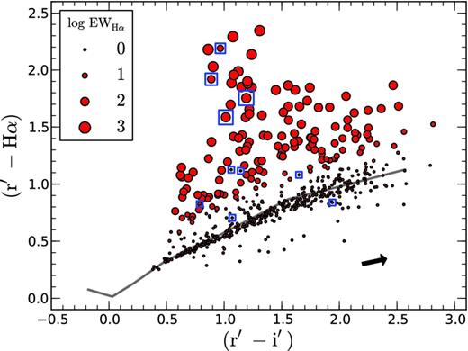
Position of objects in the IPHAS (r′ − i′)/(r′ − Hα) plane. The size of the circles represents the expectation value of the Hα EW posterior. The solid line shows the unreddened main sequence, while the arrow shows the typical reddening vector for a unit AV, both taken from Paper I. Blue squares indicate objects with low likelihoods (cf. Section 5.3).
Secondly, Fig. 12 shows the (r′ − i′)/(i′ − J) plane. In this diagram, we let the size of the symbols represent the extinction estimate because the unit reddening vector (black arrow) follows a direction which is somewhat offset from the main locus of stars, such that objects with high extinction tend to be located above the main locus.
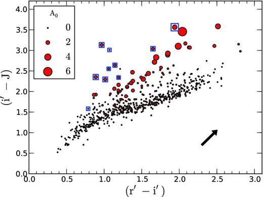
Position of objects in the IPHAS–2MASS (r′ − i′)/(i′ − J) plane. The size of the circles represents the mean extinction posterior. The arrow shows the reddening vector for AV = 1 due to Schlegel et al. (1998).
At first glance, this diagram shows a good agreement between the position of objects and their estimated extinction. However, we draw the reader's attention to the lack of a one-on-one relationship between the extinction and the apparent distance from the main locus. As discussed in Section 2.1.2, this is a result of the fact that the Hα line falls inside the r′ band, which has the effect of moving emission-line objects towards the left of the diagram and above the main locus, such that strong Hα emitters with low extinction occupy the same region in the diagram as objects with weak emission and high extinction. This illustrates the fact that it is difficult to simultaneously estimate extinction and Hα emission from these diagrams, which was a major motivation for adopting the Bayesian approach (cf. Section 2).
Finally, Fig. 13 shows the (r′ − i′)/r′ plane, which can be used to trace the ages and masses in a way similar to a Hertzsprung–Russell diagram. The objects shown in this plane have been dereddened according to their individual extinction estimates, such that we can compare their position against the theoretical isochrones (dashed lines) and evolutionary mass tracks (dotted lines) from the Siess et al. model. We find a good agreement between the position of objects in the diagram and their estimated masses. An equally good agreement is found for the age estimates (not shown).
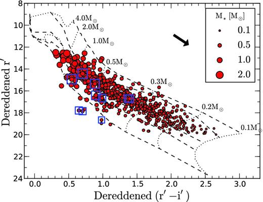
Position of objects in the IPHAS (r′ − i′)/r′ plane, dereddened using the mean extinction posterior values of each object. The size of the circles represents the mean stellar mass posterior. The arrow shows the reddening vector for a unit AV due to Schlegel et al. (1998). We also show the evolutionary mass tracks (dotted lines) and isochrones (dashed lines) from the Siess et al. model, placed at the adopted distance of 760 pc. The isochrones are for 0.1, 1, 5, 10 and 100 Myr (top to bottom).
5.2 Comparison with existing spectroscopy
The most comprehensive set of spectroscopy towards NGC 2264 that is currently available in the literature is the survey presented by Dahm & Simon (2005), which is based on the Wide-Field Grism Spectrograph (WFGS) on the University of Hawaii 2.2-m telescope on Mauna Kea, augmented with spectra from the Gemini North 8.2-m telescope.
Their data set provides spectroscopic Hα EWs for 74 out of the 115 accreting objects in our sample. We find a good correlation between their values and our estimates (r = 0.8) which is shown in Fig. 14, albeit with a significant scatter. The spread in the relationship is very similar to the one we previously found in a different cluster (Paper I), and is thought to be due to a combination of natural variability and uncertainty (the median 1σ uncertainty for our estimates is shown in the bottom right of the plot).
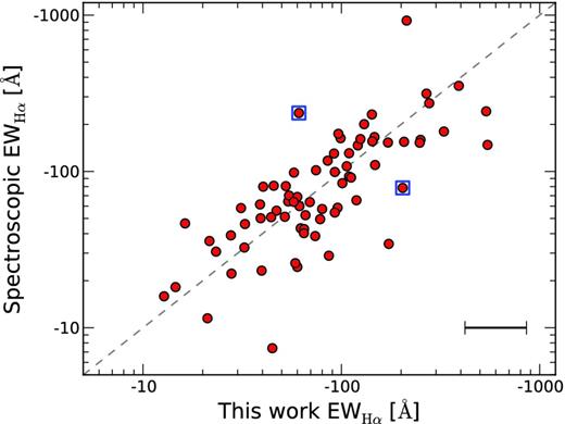
Comparison of our inferred Hα EWs with values obtained from grism spectroscopy by Dahm & Simon (2005). The grey dashed line shows the unity relation. The median error bar is shown in the bottom right. The scatter is thought to be due to a combination of uncertainty and natural Hα emission variability.
We note that the work by Dahm & Simon highlighted the strong natural variability of the Hα line. Using spectra from multiple epochs between 1990 and 2003, the authors reported that nearly all of the CTTS (90 per cent) exhibited changes in the EW at or above the 10 per cent level, while 57 per cent varied at 50 per cent or greater. This confirms that the scatter is at least in part due to natural variability.
5.3 Objects with low likelihoods
An advantage of the Bayesian method is that we may evaluate how well the model matches different objects by comparing their mean likelihood values (obtained from equation 28). Using this information, we found a small number of ∼10 objects with significantly lower likelihoods than the main locus of stars. These 10 ‘worst-fitting’ objects have been marked by blue rectangles in Figs 11–14 (object IDs: C13507, C22501, C27963, C28541, C31190, C31352, C33877, C36198, C36493 and C37366).
The markers reveal that several of these objects show strong Hα emission in Fig. 11, while the colours appear anomalous in Fig. 12, where they fall beyond the extreme blue edge of the locus. Likewise, a few fall below the main locus in Fig. 13.
We can think of four reasons to explain their position.
The objects might be blue Hα emitters in the background, e.g. interacting binaries, Be stars or unresolved planetary nebulae (Corradi et al. 2008) not related to NGC 2264.
If the objects are genuine members, the presence of strong Hα emission suggests that they are undergoing high levels of mass accretion, which is known to be a cause for continuum veiling in the red part of the spectrum. The origin of such emission is unclear however (Fischer et al. 2011).
The objects might be affected by anomalous extinction. Three of the stars have previously been discussed by Sung et al. (2008, 2009) who classified them as ‘BMS’ (for below the pre-main sequence) based on their outlier position in the colour–magnitude diagram. Sung et al. supported the assumption that these are bona-fide young stars with a nearly edge-on disc. The dust grains in a disc tend to be larger than those in the interstellar medium, and hence the extinction law may differ significantly.
It is possible that the edge of the disc contaminates the colours of the star, depending on the inner radius, inclination and shape of the disc.
If these outlier objects are genuine members, they provide evidence that our results would profit from a more advanced pre-main-sequence model which includes the effects of continuum veiling due to accretion and dust in the circumstellar environment. We will discuss this prospect in Section 6.
5.4 The extinction prior
We noted previously that the extinction distribution (Fig. 10c) shows a deficit of highly reddened objects when compared to the prior (blue solid line). The prior was chosen based on the distribution of spectroscopy-based extinctions determined by Rebull et al. (2002) for 202 candidate members (Section 2).
The mismatch between our results and the prior is explained by the use of different selection criteria in both studies. On the one hand, the membership selection by Rebull et al. made use of a combination of colour–magnitude diagrams and photometric variability, which is prone to the inclusion of background objects (i.e. out of the 17 objects for which the authors reported extinctions larger than |${A_{\rm V}}> 3$|, only two passed our membership criteria). On the other hand, the use of optical photometry and X-ray observations in our criteria is likely to introduce a bias against highly reddened objects.
The mismatch illustrates that the extinction prior does not determine the results alone, but merely helps the data to constrain the parameters using the additional knowledge which we chose to include. To understand the influence of the prior, we repeated the inference procedure using a log-uniform prior P(log A0) |$\sim \mathcal {U}(-1, 1)$|, which is less informed. We found this prior to produce near-identical results with mean log A0 = −0.32 (A0 = 0.48), which differs from the original mean extinction by only +0.05 mag. The influence of this prior on the other parameters was found to be negligible, with mass estimates showing a median shift of +0.01 M⊙ and the median age remaining constant.
We also repeated the experiment using the absolute uniform prior P(A0) |$\sim \mathcal {U}(0, 10)$|, which favours high extinctions far more strongly than the log-uniform prior. This was found to change the extinction of individual objects by a factor of 2.1 on average, hence raising the mean extinction of the sample to log A0 = −0.03 (A0 = 0.93). As a result, masses experienced a median shift of +0.11 M⊙ and the median age increased from 3.0 to 4.3 Myr.
The factor ∼2 corresponds to the typical 1σ uncertainty in the extinction of highly reddened objects in our results (e.g. Fig. 6). We therefore estimate that this is the level at which our method is able to constrain the extinction in regions where no prior information is available. The ability to constrain the extinction within a factor of ∼2 meets the level of accuracy we may reasonably expect from the combination of r′/i′/J magnitudes, and represents a significant improvement over the widely used practice of assuming a fixed extinction value in the absence of spectroscopic data. Moreover, we are confident that including additional photometry at longer wavelengths (e.g. 2MASS H/K) can further strengthen our handle on the extinction in future work.
6 FUTURE EXTENSIONS
We envisage extending the method presented in this work on two fronts: (i) more comprehensive modelling of the individual stars and (ii) modelling the global properties of the cluster.
First, in the previous section we found indications that our results would profit from a more detailed model of T Tauri stars, which should include the effects of continuum veiling due to accretion shocks, as well as the presence of dust in the circumstellar environment. We envisage employing a grid of radiation transfer models for this purpose, such as the widely used models by Robitaille et al. (2006, 2007). We note that a maximum-likelihood fitting tool already exists for these models.3 At present the tool only links observations to ‘best-fitting’ parameters however, and it does not reveal the full posterior. In turn, a more detailed model invites the inclusion of photometry across a wider wavelength range. We note the possibility to include U- and g-band magnitudes from the UV-excess (UVEX) and VPHAS galactic plane surveys (Groot et al. 2009), deep JHK magnitudes from the UKIDSS surveys (Lucas et al. 2008) and infrared photometry from space-based telescopes.
Secondly, in Section 4 we explained that our findings on the global properties of NGC 2264 must be interpreted with caution because we did not incorporate the cluster properties as part of our probabilistic model. This would be desirable because there are pertinent open issues in the current literature which require a careful treatment of the parameter uncertainties (these questions include the ages of clusters, their age spreads and the dependency of accretion rates on stellar masses, e.g. see Clarke & Pringle 2006; Jeffries et al. 2011). These questions may be addressed by adding the relevant cluster parameters to the top of the hierarchical model in Fig. 3.
It is worth emphasizing that the goal of understanding clusters can be regarded as the problem of finding a hierarchical model which best explains the observations. For this reason, we encourage others to adopt graphical Bayesian models as a generic framework to link observations to theory.
7 CONCLUSIONS
We showed how the theory of graphical Bayesian networks can be used to define a probabilistic model which allows extinction, age, mass and accretion rate to be inferred from IPHAS r′/Hα/i′ and 2MASS J-band photometry without the need for spectroscopy. The model combined the evolutionary model due to Siess et al. (2000) and the simulated photometry for Hα emission-line stars due to Barentsen et al. (2011a) to compute probabilistic posterior distributions.
Compared to more popular plane-fitting or maximum-likelihood techniques, the advantages of our approach are that (i) we dealt with the degeneracy between stellar mass and extinction by considering the full probability distribution of solutions and (ii) we obtained meaningful expectation values and uncertainties by marginalizing over nuisance parameters such as the distance and disc truncation radius.
We used the python/pymc library to compute the model using an MCMC algorithm, which was found to take only a small amount of programming effort (Appendix A). We then applied the method to 587 low-mass members of the NGC 2264 star-forming region and found a good agreement between our results and the position of stars in colour–magnitude diagrams, as well as literature spectroscopy. We performed an initial inspection of the sample and found the following.
NGC 2264 shows a median age of 3.0 Myr, albeit with a large apparent dispersion between 1.8 and 4.5 Myr (25 and 75 per cent quartiles).
115 objects (20 ± 2 per cent) show fractional Hα luminosities above the chromospheric saturation limit (log LHα/L* > −3.3; Barrado y Navascués & Martín 2003) and are therefore very likely to be CTTS objects which are accreting gas from a circumstellar disc.
For these CTTS objects, we estimated mass accretion rates on the basis of Hα luminosities and found them to range between 10−10.7 and 10−6.4 M⊙ yr−1 with a median of 10−8.4 M⊙ yr−1.
The results were shown to be consistent with existing spectroscopic studies in the literature. Our method achieved these results with great efficiency by depending only on photometry, and provides a significant step forward from previous photometric methods because our probabilistic approach ensures that nuisance parameters, such as extinction and distance, are fully included in the analysis with a clear picture on any degeneracies.
In future work, we envisage extending the method to include more physics. We note the possibility to utilize a grid of radiation transfer models which include the effects of continuum veiling and material in the circumstellar environment. In turn, our method would benefit from the inclusion of additional photometric bands across a wider wavelength range.
Graphical Bayesian models provide a generic framework for estimating parameters from sparse data. We expect that the approach will become increasingly important as a tool for the effective utilization of large surveys, in particular once distance estimates from Gaia can be included. We remind the reader that our source code is made available online4 and encourage others to reuse or improve the code.
We thank Nick Wright, Eduardo Martin, Eli Bressert, Christian Knigge, Roberto Raddi, Renko and Thomas Barclay for constructive comments which helped to improve the paper. We thank David W. Hogg for getting us to adopt probabilistic inference through his blog and talks. We thank the referee, Frédéric J. Pont, for insightful corrections which strengthened the paper.
Armagh Observatory is funded by major grants from the Department of Culture, Arts and Leisure (DCAL) for Northern Ireland and the UK Science and Technology Facilities Council (STFC). The IPHAS survey is carried out at the Isaac Newton Telescope (INT), operated by the Isaac Newton Group in the Spanish Observatorio del Roque de los Muchachos of the Instituto de Astrofisica de Canarias. IPHAS data were processed by the Cambridge Astronomical Survey Unit at the Institute of Astronomy in Cambridge. 2MASS is a joint project of the University of Massachusetts and IPAC/Caltech, funded by NASA/NSF.
Our work made use of topcat (Taylor 2005), aladin, postgresql, python (pymc, pyfits, aplpy modules) and amazon ec2. Mosaics were generated using the montage software maintained by NASA/IPAC.
REFERENCES
APPENDIX A: python source code for the inference model


SUPPORTING INFORMATION
Additional Supporting Information may be found in the online version of this article:
Table 3. IPHAS and 2MASS photometry for known members of NGC 2264 which satisfy our selection and quality criteria.
Table 4. Posterior expectation values and standard deviations for parameters of NGC 2264 members, obtained from IPHAS and 2MASS photometry using Bayesian inference (Supplementary Data).
Please note: Oxford University Press are not responsible for the content or functionality of any supporting materials supplied by the authors. Any queries (other than missing material) should be directed to the corresponding author for the article.
