


Abstract
The spatial distribution of gas matter inside galaxy clusters is not completely smooth, but may host gas clumps associated with substructures. These overdense gas substructures are generally a source of unresolved bias of X-ray observations towards high-density gas, but their bright luminosity peaks may be resolved sources within the intra cluster medium (ICM), that deep X-ray exposures may be (already) capable to detect. In this paper we aim at investigating both features, using a set of high-resolution cosmological simulations with enzo. First, we monitor how the bias by unresolved gas clumping may yield incorrect estimates of global cluster parameters and affects the measurements of baryon fractions by X-ray observations. We find that based on X-ray observations of narrow radial strips, it is difficult to recover the real baryon fraction to better than 10–20 per cent uncertainty. Secondly, we investigated the possibility of observing bright X-ray clumps in the nearby Universe (z ≤ 0.3). We produced simple mock X-ray observations for several instruments (XMM, Suzaku and ROSAT) and extracted the statistics of potentially detectable bright clumps. Some of the brightest clumps predicted by simulations may already have been already detected in X-ray images with a large field of view. However, their small projected size makes it difficult to prove their existence based on X-ray morphology only. Preheating, active galactic nuclei feedback and cosmic rays are found to have little impact on the statistical properties of gas clumps.
1 INTRODUCTION
The properties of gas matter in more than two-thirds of the galaxy cluster volume are still largely unknown. In order to further improve our use of clusters as high-precision cosmological tools, it is therefore necessary to gain insight into the thermodynamics of their outer regions (see Ettori & Molendi 2011, and references therein). The surface brightness distribution in clusters outskirts has been studied with ROSAT (e.g. Eckert et al. 2012, and references therein) and with Chandra (see Ettori & Balestra 2009, and references therein). A step forward has been the recent observation of a handful of nearby clusters with the Japanese satellite Suzaku that, despite the relatively poor point spread function (PSF) and small field of view of its X-ray imaging spectrometer (XIS), benefits from the modest background associated with its low-Earth orbit (see results on PKS0745-191, George et al. 2009; A2204, Reiprich et al. 2009; A1795, Bautz et al. 2009; A1413, Hoshino et al. 2010; A1689, Kawaharada et al. 2010; Perseus, Simionescu et al. 2011; Hydra A, Sato et al. 2012; see also Akamatsu & Kawahara 2011). The first results from Suzaku indicate a flattening and sometimes even an inversion of the entropy profile moving outwards. The infall of cool gas from the large-scale structure might cause the assumption of hydrostatic equilibrium to break down in these regions, which could have important implications on cluster mass measurements (Rasia, Tormen & Moscardini 2004; Lau, Kravtsov & Nagai 2009; Burns, Skillman & O’Shea 2010). However, as a consequence of the small field of view (and of the large solid angle covered from the bright nearby clusters) observations along a few arbitrarily chosen directions often yield very different results.
In addition to instrumental effects (e.g. Eckert et al. 2011), or non-gravitational effects (e.g. Roncarelli et al. 2006; Battaglia et al. 2010; Lapi, Fusco-Femiano & Cavaliere 2010; Mathews & Guo 2011; Bode et al. 2012; Vazza et al. 2012), there are ‘simpler’ physical reasons to expect that properties of the ICM derived close to ∼R200 may be more complex than what is expected from idealized cluster models.
One effect is cluster triaxiality and asymmetry, which may cause variations in the ICM properties along directions, due to the presence of large-scale filaments in particular sectors of each cluster (e.g. Vazza et al. 2011c; Eckert et al. 2012), or to the cluster-to-cluster variance related to the surrounding environment (e.g. Burns et al. 2010).
A second mechanism related to simple gravitational physics is gas clumping, and its possible variations across different directions from the cluster centre (Mathiesen, Evrard & Mohr 1999; Nagai & Lau 2011).
In general, gas clumping may constitute a source of uncertainty in the derivation of properties of galaxy cluster atmospheres since a significant part of detected photons may come from the most clumpy structures of the ICM, which may not be fully representative of the underlying large-scale distribution of gas (e.g. Roncarelli et al. 2006; Vazza et al. 2011c). Indeed, a significant fraction of the gas mass in cluster outskirts may be in the form of dense gas clumps, as suggested by recent simulations (Nagai & Lau 2011). In such clumps the emissivity of the gas is high, leading to an overestimation of the gas density if the assumption of constant density in each shell is made. The recent results of Nagai & Lau (2011) and Eckert et al. (2012) show that the treatment of gas clumping factor slightly improves the agreement between simulations and observed X-ray profiles.
The gas clumping factor can also bias the derivation of the total hydrostatic gas mass in galaxy clusters at the ∼10 per cent level (Mathiesen et al. 1999), and it may as well bias the projected temperature low (Rasia et al. 2005). Theoretical models of active galactic nuclei (AGN) feedback also suggest that overheated clumps of gas may lead to a more efficient distribution of energy within cluster cores (Birnboim & Dekel 2011).
Given that the effect of gas clumping may be resolved or unresolved by real X-ray telescopes depending on their effective resolution and sensitivity, in this paper we aim at addressing both kind of effects, with an extensive analysis of a sample of massive (∼1015 M⊙) galaxy clusters simulated at high spatial and mass resolution (Section 2). First, we study in Section 3.1 the bias potentially present in cluster profiles derived without resolving the gas substructures. Secondly, in Section 3.2 we derive the observable distribution of X-ray bright clumps, assuming realistic resolution and sensitivity of several X-ray telescopes. We test the robustness of our results with changing resolution and with additional non-gravitational processes [radiative cooling, cosmic rays (CRs), AGN feedback] in Section 3.3. Our discussion and conclusions are given in Section 4.
2 CLUSTER SIMULATIONS
The simulations analysed in this work were produced with the Adaptive Mesh Refinement code ENZO 1.5, developed by the Laboratory for Computational Astrophysics at the University of California in San Diego1 (e.g. Norman et al. 2007; Collins et al. 2010, and references therein). We simulated 20 galaxy clusters with masses in the range 6 × 10¹⁴ ≤ M/M⊙ ≤ 3 × 10¹⁵, extracted from a total cosmic volume of Lbox ≈ 480 Mpc h−1. With the use of a nested grid approach we achieved high mass and spatial resolution in the region of cluster formation: mdm = 6.76 × 10⁸ M⊙ for the dark matter (DM) particles and ∼25 kpc h−1 in most of the cluster volume inside the ‘AMR region’ (i.e. ∼2–3 R200 from the cluster centre; see Vazza et al. 2010, 2011; Vazza 2011 for further details).
We assumed a concordance Λcold dark matter cosmology, with Ω0 = 1.0, ΩB = 0.0441, ΩDM = 0.2139, ΩΛ = 0.742, Hubble parameter h = 0.72 and a normalization for the primordial density power spectrum of σ8 = 0.8. Most of the runs we present in this work (Sections 3.1– 3.2) neglect radiative cooling, star formation and AGN feedback processes. In Section 3.3, however, we discuss additional runs where the following non-gravitational processes are modelled: radiative cooling, thermal feedback from AGN, and pressure feedback from CR particles injected at cosmological shock waves.
For consistency with our previous analysis on the same sample of galaxy clusters (Vazza et al. 2010, 2011a,c), we divided our sample in dynamical classes based on the total matter accretion history of each halo for z ≤ 1.0. First, we monitored the time evolution of the DM+gas mass for every object inside the ‘AMR region’ in the range 0.0 ≤ z ≤ 1.0. Considering a time lapse of Δt = 1 Gyr, ‘major merger’ events are detected as total matter accretion episode where M(t + Δt)/M(t) − 1 > 1/3. The systems with a lower accretion rate were further divided by measuring the ratio between the total kinetic energy of gas motions and the thermal energy inside the virial radius at z = 0, since this quantity parameter provides an indication of the dynamical activity of a cluster (e.g. Tormen, Bouchet & White 1997; Vazza et al. 2006). Using this proxy, we defined as ‘merging’ systems those objects that present an energy ratio >0.4, but did not experience a major merger in their past (e.g. they show evidence of ongoing accretion with a companion of comparable size, but the cores of the two systems did not encounter yet). The remaining systems were classified as ‘relaxed’. According to the above classification scheme, our sample presents four relaxed objects, six merging objects and 10 post-merger objects.
Based on our further analysis of this sample, this classification actually mirrors a different level of dynamical activity in the subgroups, i.e. relaxed systems on average host weaker shocks (Vazza et al. 2010); they are characterized by a lowest turbulent to thermal energy ratio (Vazza et al. 2011a) and they are characterized by the smallest amount of azimuthal scatter in the gas properties (Vazza et al. 2011c; Eckert et al. 2012). In Vazza et al. (2011c) the same sample was also divided based on the analysis of the power ratios from the multi-pole decomposition of the X-ray surface brightness images (P3/P0), and the centroid shift (w), as described by Böhringer et al. (2010). These morphological parameters of projected X-ray emission maps were measured inside the innermost projected 1 Mpc2. This leads to decompose our sample into nine ‘non-cool-core-like’ (NCC) systems, and 11 ‘cool-core-like’ systems (CC), once that fiducial thresholds for the two parameters (as in Cassano et al. 2010) are set. We report that (with only one exception) the NCC-like class here almost perfectly overlaps with the class of post-merger systems of Vazza et al. (2010), while the CC-like class contains the relaxed and merging classes of Vazza et al. (2010).
Table 1 lists of all simulated clusters, along with their main parameters measured at z = 0. All objects of the sample have a final total mass >6 × 10¹⁴ M⊙, 12 of them having a total mass >1015 M⊙. In the last column, we give the classification of the dynamical state of each cluster at z = 0, and the estimated epoch of the last major merger event (for post-merger systems).
Main characteristics of the simulated clusters at z = 0. Column 1: identification number; 2: total virial mass (Mvir = MDM + Mgas); 3: virial radius (Rv); 4: dynamical classification: RE = relaxing, ME = merging or MM = major merger; 5: approximate redshift of the last merger event.
| ID | Mvir | Rv | Dynamical state | Redshift |
|---|---|---|---|---|
| (1015 M⊙) | (Mpc) | (zMM) | ||
| E1 | 1.12 | 2.67 | MM | 0.1 |
| E2 | 1.12 | 2.73 | ME | – |
| E3A | 1.38 | 2.82 | MM | 0.2 |
| E3B | 0.76 | 2.31 | ME | – |
| E4 | 1.36 | 2.80 | MM | 0.5 |
| E5A | 0.86 | 2.39 | ME | – |
| E5B | 0.66 | 2.18 | ME | – |
| E7 | 0.65 | 2.19 | ME | – |
| E11 | 1.25 | 2.72 | MM | 0.6 |
| E14 | 1.00 | 2.60 | RE | – |
| E15A | 1.01 | 2.63 | ME | – |
| E15B | 0.80 | 2.36 | RE | – |
| E16A | 1.92 | 3.14 | RE | – |
| E16B | 1.90 | 3.14 | MM | 0.2 |
| E18A | 1.91 | 3.14 | MM | 0.8 |
| E18B | 1.37 | 2.80 | MM | 0.5 |
| E18C | 0.60 | 2.08 | MM | 0.3 |
| E21 | 0.68 | 2.18 | RE | – |
| E26 | 0.74 | 2.27 | MM | 0.1 |
| E62 | 1.00 | 2.50 | MM | 0.9 |
2.1 X-ray emission
We simulated the X-ray flux (SX) from our clusters, assuming a single temperature plasma in ionization equilibrium within each 3D cell. We use the Astrophysical Plasma Emission Code (APEC) emission model (e.g. Smith et al. 2001) to compute the cooling function Λ(T, Z) (where T is the temperature and Z the gas metallicity) inside a given energy band, including continuum and line emission. For each cell in the simulation we assume a constant metallicity of Z/Z⊙ = 0.2 (which is a good approximation of the observed metal abundance in cluster outskirts; Leccardi & Molendi 2008). While line cooling may be to the first approximation not very relevant for the global description of the hot ICM phase (T ∼ 108 K), it may become significant for the emission from clumps, because their virial temperature can be lower than that of the host cluster by a factor of ∼10. Once the metallicity and the energy band are specified, we compute for each cell the X-ray luminosity, SX = nHneΛ(T, Z) dV, where nH and ne are the number density of hydrogen and electrons, respectively, and dV is the volume of the cell.
2.2 Definition of gas clumps and gas clumping factor
Although the notion of clumps and of the gas clumping factor is often used in the recent literature, an unambiguous definition of this is non-trivial.2 In this work we distinguish between resolved gas clumps (detected with a filtering of the simulated X-ray maps) and unresolved gas clumping, which we consider as an unavoidable source of bias in the derivation of global cluster parameters from radial profiles. On the theoretical point of view, gas clumps represent the peaks in the distribution of the gas clumping factor, and can be identified as single ‘blobs’ seen in projection on the cluster atmosphere if they are bright enough to be detected. While resolved gas clumps are detected with a 2D filtering of the simulated X-ray images (based on their brightness contrast with the smooth X-ray cluster emission), the gas clumping factor is usually estimated in the literature within radial shells from the cluster centre. The two approaches are not fully equivalent, and in this paper we address both, showing that in simple non-radiative runs they are closely related phenomena, and present similar dependence on the cluster dynamical state.
2.2.1 Resolved gas clumps
We identify bright gas clumps in our cluster sample by post-processing 2D mock observations of our clusters. We do not consider instrumental effects of real observations (e.g. degrading spatial resolution at the edge of the field of view of observation), in order to provide the estimate of the theoretical maximum amount of bright gas clumps in simulations. Instrumental effects depend on the specific features of the different telescope, and are expected to further reduce the rate of detection of such X-ray clumps in real observations. In this section we show our simple technique to preliminary extract gas substructures in our projected maps, using a rather large-scale (300 kpc h−1). ‘X-ray bright gas clumps’, in our terminology, correspond to the observable part of these substructures, namely their small (≤50 kpc h−1) compact core, which may be detected within the host cluster atmosphere according the effective resolution of observations (Section 3.2).
Based on the literature (e.g. Dolag et al. 2005, 2009), the most massive substructures in the ICM have a (3D) linear scale smaller than <300–500 kpc h−1. We investigated the typical projected size of gas substructures by computing the 2D power spectra of SX for our cluster images. In order to remove the signal from the large-scale gas atmosphere we subtracted the average 2D cluster profile from each map. We also applied a zero-padding to take into account the non-periodicity of the domain (see Vazza et al. 2011a and references therein). The results are shown in Fig. 1 for three representative clusters of the sample at z = 0: the relaxed cluster E15B, the post-merger cluster E1 and the merging system E3B merging (see also Fig. 2). The long-dashed profiles show the power spectra of the X-ray image of each cluster, while the solid lines show the spectra after the average 2D profile of each image has been removed. The power spectra show that most of the residual substructures in X-ray are characterized by a spatial frequency of k > 10–20, corresponding to typical spatial scales l0 < 300–600 kpc h−1, similar to 3D results (Dolag et al. 2009). A dependence on the dynamical state of the host cluster is also visible from the power spectra: the post-merger and the merging clusters have residual X-ray emission with more power also on smaller scales, suggesting the presence of enhanced small-scale structures in such systems. We will investigate this issue in more detail in the following sections.
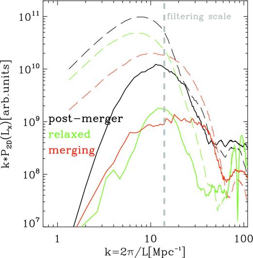
2D power spectra of X-ray maps for three simulated clusters at z = 0 (E1, E3B and E15B, as in Fig. 2). Only one projection is considered. The long-dashed lines show the power spectra of the total X-ray image of each cluster, while the solid lines show the spectrum of each image after the average X-ray profile has been removed. Zero-padding has been considered to deal with the non-periodic domain of each image. The spectra are given in arbitrary code units, but the relative difference in normalization of each cluster spectrum is kept. The vertical grey line shows our filtering scale to extract X-ray clumps within each image.
![Top panels: X-ray flux in the (0.5–2) keV (in [erg (s cm−2)]) of three simulated clusters of our sample at z = 0 (E15B-relax, E1-post merger and E3B merging). Bottom panels: X-ray flux of clumps identified by our procedure (also highlighted with white contours). The inner and outer projected area excluded from our analysis has been shadowed. The area shown within each panel is ∼3 × 3 R200 for each object.](https://oup.silverchair-cdn.com/oup/backfile/Content_public/Journal/mnras/429/1/10.1093/mnras/sts375/2/m_sts375fig2.jpeg?Expires=1750221962&Signature=QahQ2eUG-dzn5cwwaMdvgoKHomKrKfNDLM8eywAultYD8SAFrLWltCuFTjhjWNExUIL5AyrIZ9rCVqO62iK-LKhqfF1O2TIrb3u12PzE-eUqYjoot0bKxLIpWR7NjWT9nIWzf5uqWGoVLBOYcotzP7xo2gpR8z7zkwm1wdcCrtzqJdlaCMClmgG1JzZqHhLKG4~QYcvlnjL4Ka9tLNgHiAIdZmg9raKQfAhqiOKeVLJOCE-DEbY6Xca~EAnHlKGhx2gDaDT1V8T9W~aT3aPtpDbtMZjLR8lLn~MMzNfSoTiXAElIF1y7Ie6HKAIYHmlaCJjKYdsPFoMelYFdNO7PDA__&Key-Pair-Id=APKAIE5G5CRDK6RD3PGA)
Top panels: X-ray flux in the (0.5–2) keV (in [erg (s cm−2)]) of three simulated clusters of our sample at z = 0 (E15B-relax, E1-post merger and E3B merging). Bottom panels: X-ray flux of clumps identified by our procedure (also highlighted with white contours). The inner and outer projected area excluded from our analysis has been shadowed. The area shown within each panel is ∼3 × 3 R200 for each object.
To study the fluctuations of the X-ray flux as a result of the gas clumps we compute maps of residuals with respect to the X-ray emission smoothed over the scale l0. The map of clumps is then computed with all pixels from the map of the residuals, where the condition SX/SX, smooth > α is satisfied. By imposing l0 = 300 kpc h−1 (∼12 cells) and α = 2, all evident gas substructures in the projected X-ray images are captured by the algorithm. We verified that the adoption of a larger or a smaller value of l0 by a factor of ∼2 does not affect our final statistics (Section 3.2) in a significant way. In Fig. 2 we show the projected X-ray flux in the [0.5-2] keV energy range from three representative clusters of the sample (E1-post merger, E3B merging and E15B relaxed, in the top panels) at z = 0, and the corresponding maps of clumps detected by our filtering procedure (lower panels). The visual inspection of the maps shows that our filtering procedure efficiently removes large-scale filaments around each cluster, and identifies blob-like features in the projected X-ray map. The relaxed system shows evidence of enhanced gas clumping along its major axis, which is aligned with the surrounding large-scale filaments. Indeed, although this system is a relaxed one based on its X-ray morphology within R200/2 [based on the measure of X-ray morphological parameters (Cassano et al. 2010), and to its very low value of gas turbulence (Vazza et al. 2011a)], its large-scale environment shows ongoing filamentary accretions and small satellites, which is a rather common feature even for our relaxed cluster outside R500. The presence of clumps in the other two systems is more evident, and they have a more symmetric distributions. We will quantify the differences of the gas clumping factor and of the distribution of bright clumps in these systems in the following sections.
2.2.2 The gas clumping factor
3 RESULTS
3.1 Gas clumping factor from large-scale structures
The average clumping factor of gas in clusters is a parameter adopted in the theoretical interpretation of de-projected profiles of gas mass, temperature and entropy (e.g. Simionescu et al. 2011; Urban et al. 2011; Eckert et al. 2012; Walker et al. 2012).
For each simulated cluster, we compute the profile of the gas clumping factor following Section 2.2.2.
Fig. 3 shows the average profile of Cρ(R) for the three dynamical classes into which our sample can be divided. The trends for all classes are qualitatively similar, with the average clumping factor Cρ < 2 across most of the cluster volume, and increasing to larger values (Cρ ∼ 3–5) outside R200. Post-merger and merging systems present a systematically larger average value of gas clumping factor at all radii, and also a larger variance within the subset. These findings are consistent with the recent results of Nagai & Lau (2011). By extracting the distribution of bright gas clumps in projected cluster images, we will see in Section 3.2 that both the radial distribution of clumps, and the trend of their number with the cluster dynamical state present identical behaviour of the gas clumping factor measured here. This again supports the idea that the two phenomena are closely associated mechanism, following the injection of large-scale substructures in the ICM.
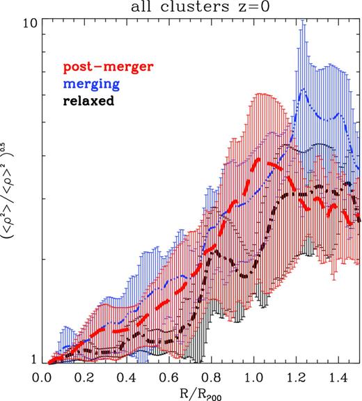
Profile of azimuthally averaged gas clumping factors for the sample of simulated clusters at z = 0 (the error bars show the 1σ deviation). The different colours represent the three dynamical classes in which we divide our sample (four relaxed, six merging and 10 post-merger clusters).
Next, we calculate the average profiles of gas clumping factor for different bins of gas over-density and temperature (limiting to the relaxed and the merging subset of clusters). This way we can determine if the gas clumping factor affects all phases of the ICM equally.
In Fig. 4 we show the average profiles of gas clumping factor calculated within different bins of gas overdensity [δρcr, b < 50, 50 ≤ δρcr, b < 102, 102 ≤ δρcr, b < 103 and δρcr, b ≥ 103, where δρcr, b is ρ/(fbρcr), with fb cosmic baryon fraction and ρcr the cosmological critical density] and gas temperature (T < 106 K, 106 ≤ T < 107 K, 107 ≤ T < 108 K and T ≥ 108 K) at z = 0.
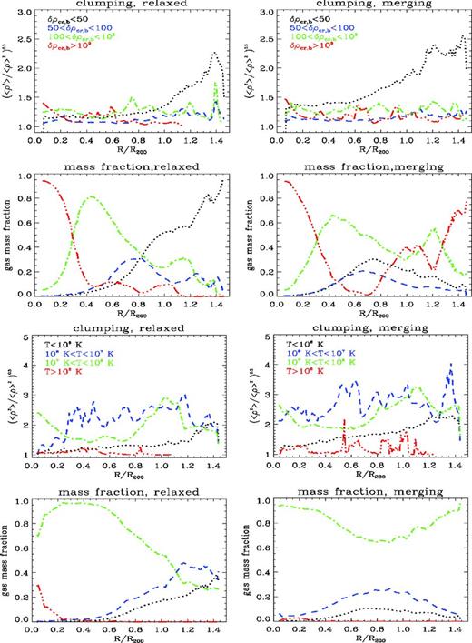
Average profiles of gas clumping factor and gas mass distribution for different phases across the whole cluster sample at z = 0, for relaxed clusters (left-hand panels) and for merging clusters (right-hand panels). The average gas clumping factor is computed for different decompositions of the cluster volume in gas-density bins (top four panels; lines are colour-coded as described in the legend in the top two panels) and temperature bins (bottom four panels are colour-coded as detailed in panels in the third row). The gas overdensity is normalized to the cosmological critical baryon density.
We want to have a characterization of the environment associated with the most significant source of gas clumping (e.g. gas substructures) in a way which is unbiased by their presence. This is non-trivial, because if the local overdensity is computed within a scale smaller than the typical size of substructures (≤300 kpc h−1), the gas density of a substructure will bias the estimate of local overdensity high. For this reason, the local gas overdensity and gas temperature in Fig. 4 have been computed for a much larger scale, 1 Mpc/h.3 In Fig. 4 we also show the gas mass fraction of each phase inside the radial shells. The gas phases show evidence that the increased clumping factor of merging clusters is related to the increased clumping factor of the low-density phase, at all radii, even if the mass of this component is not dominant in merging systems. An increased clumping factor is also statistically found in the cold (<106 K) and intermediate 106 ≤ T < 107 phase of gas in merging systems. We remark that although the increase in this phase is associated with an enhanced presence of X-ray detectable clumps (Section 3.2), it cannot be directly detected in X-ray, due to its low emission temperature.
The gas phase characterized by δρcr, b < 50 and T ≤ 106–107 is typical of large-scale filaments (Dolag, Bykov & Diaferio 2008; Vazza, Brunetti & Gheller 2009; Iapichino et al. 2011). While filaments only host a small share of the gas mass inside the virial radius, they can dominate the clumping factor within the entire volume of the merging systems. This is because their gas matter content contains significantly more clumpy matter compared to the ICM on to which they accrete. This suggests that a significant amount of gas substructure (e.g. including massive and bright X-ray clumps, as in Section 3.2) can originate from low-density regions, and not necessarily from the hot and dense phase of the ICM. This is reasonable in the framework of hierarchical structure formation, since matter inside filaments had almost the entire cosmic evolution to develop substructures (Einasto et al. 2011). Contrary to most of the matter inside galaxy clusters, large-scale filaments have never undergone a phase of violent relaxation and efficient mixing. Therefore, even at late cosmic epochs they can supply very clumpy material. This suggests that clusters in an early merging phase are characterized by the largest amount of gas clumping factor at all radii, and that this clumpy material is generally associated with substructures coming from filaments and from the cluster outskirts. Filaments between massive galaxy clusters are indeed found to anticipate major mergers in simulations (Vazza et al. 2011a), starting the injection of turbulence in the ICM already some ∼ Gyr before the cores-collision.
We now investigate how gas clumping can affect X-ray observations. For this purpose, we compare in Fig. 5 the real profiles of clumping factor, DM, gas density and baryon fraction for the same clusters as in Fig. 2, with profiles derived from the entire cluster volume or within smaller volumes (i.e. thin slices along the line of sight) along perpendicular sectors of the same systems. All profiles are drawn from the centre of total (gas+DM) mass of each system. These selected volumes are meant to broadly compare with the selection of sectors chosen in recent deep X-ray observations of clusters (Simionescu et al. 2011; Urban et al. 2011; Humphrey et al. 2012). Therefore, in this case we studied the radial profiles inside rectangular sectors of width ∼500 kpc, similar to observations (Simionescu et al. 2011; Urban et al. 2011), and the largest available line of sight (∼8 Mpc). The projected total volume sampled by these sectors is ∼20 per cent of the total cluster volume, and it is interesting to study how representative the information is that can be derived from them.
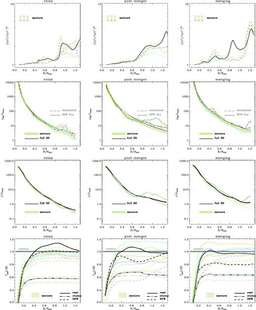
Top panels: radial profiles of clumping factor for three clusters of the sample at z = 0 (from left to right: E15B-relax, E1-post merger and E3B merging). The solid black line shows the average gas clumping factor for the whole volume, and the additional coloured lines show the gas clumping factor inside four smaller sectors from the cluster centre. Second row: radial profiles of DM density for the total volume (black) and for the sectors (colours). The dot–dashed lines show the simulated data, and the solid ones the best fit of the NFW profile for the corresponding volumes. Third row: average gas density profiles for the same volumes (same meaning of colours). Last row: profiles of enclosed gas mass fraction for the same volumes. We show the real profile (solid lines), the ‘clumpy’ baryon fraction (dot–dashed) and the ‘X-ray’ baryon fraction (dashed) for each corresponding volume.
For comparison with the observationally derived baryon fraction, we compute the best-fitting model for NFW profiles (Navarro, Frenk & White 1996) using the CURVEFIT task in IDL for the total volume, and for each sector independently. The radial range used to compute the best fit to the NFW profile is 0.02 R200 ≤ R ≤ R200.
In the relaxed system (first panels) there is little gas clumping out to a radius 0.8R200. The average profile of DM is overall well modelled by the NFW profile everywhere up to ∼R200. The profiles inside smaller sectors are also well described by a NFW profile, yet for >0.6R200 the NFW profiles within each sector start to deviate from one another. At large radii the best-fitting profiles are found to be both under- or overestimating the real DM profile, due to large-scale asymmetries in the cluster atmosphere (e.g. left-hand panel of Fig. 2). Asymmetries in this relaxed cluster also cause a similar azimuthal scatter of gas profiles, similar to what was found in Vazza et al. (2011c).
The departures from the NFW profile and the differences between sectors are significantly larger in the post-merger and the merging systems (second and third columns of Fig. 5). We find that the best-fitting NFW profiles can differ significantly between sectors, with a relative difference of up to ∼30–40 per cent at R200 in the merging system caused by the infalling second cluster (see right-hand panel of Fig. 2). In addition to azimuthal variations, also large differences (>40 per cent) between the true DM profile and the best-fitting NFW profile are found along some sectors.
These uncertainties in the ‘true’ gas/DM mass within selected sectors bias the estimated enclosed baryon fraction. This is an important effect which may provide the solution to understand the variety of recent results provided by observations (Simionescu et al. 2011; Urban et al. 2011; Humphrey et al. 2012; Walker et al. 2012).
In Fig. 5, we present the radial trend of the enclosed baryon fraction, Ygas(< R) ≡ fbar(< R)/fb for each cluster and sector (where fb is the cosmic baryon fraction), following three different approaches:
we measure the ‘true’ baryon fraction inside spherical shells (or portion of spherical shells, for the narrow sectors);
we measure the ‘X-ray-like’ baryon fraction given by |$(\int 4 \pi R^2 \rho (R)^2 \text{d}R)^{0.5}/\int 4 \pi R^2 \rho (R)_{\rm NFW}\,\, \text{d}R$|, where ρNFW is the profile given by the best-fitting NFW profile for DM (for the total volume or for each sector separately);
we measure the ‘clumpy’ baryon fraction, |$(\int 4 \pi R^2 \rho (R)^2 \text{d}R/\int 4 \pi R^2 \rho (R)_{\rm DM}^2 \text{d}R)^{0.5}$|, where ρ(R)DM is the true DM density.
This ‘clumpy’ estimate of Ygas obviously has no corresponding observable, since it involves the clumping factor of the DM distribution. However, this measure is useful because it is more connected to the intrinsic baryon fraction of the massive substructures within galaxy clusters.
The radial trend of the true baryon fraction for the total volume is in line with the result of observations (Allen, Schmidt & Fabian 2002; Vikhlinin et al. 2006; Ettori et al. 2009), with Yg increasing from very low central values up to the cosmic value close to R200. The total enclosed baryon fraction inside <1.2 R200 is ±5 per cent of the cosmic value, yet larger departures (±10–20 per cent) can be found inside the narrow sectors.
The ‘X-ray-like’ measurement of the enclosed baryon fraction is subject to a larger azimuthal scatter, and shows larger differences also with respect to the true enclosed baryon fraction. In our data sample, it rarely provides an agreement better than ±10 per cent with the true enclosed baryon fraction (considering the whole cluster or the sectors). Based on our sample, we estimate that on average in ∼25 per cent of cases the baryon fraction measured within sectors by assuming an underlying NFW profile overestimates the true baryon fraction by a ∼10 per cent, while in ∼50 per cent of cases it underestimates the cosmic baryon fraction by a slightly larger amount (∼10–20 per cent). In the remaining cases, the agreement at R200 is of the order of ∼5 per cent.
In all cases the main factor for significant differences between the X-ray-derived baryon fraction and the true one is the triaxiality of the DM matter distribution within the cluster rather than enhanced gas clumping. As an example, in the relaxed cluster of Fig. 5 the ‘X-ray’ baryon fraction is underestimated in two sectors, it is overestimated in one sector and it almost follows the true one in the last sector. This trend is mainly driven by the difference between the true DM profiles and the best-fitting NFW profiles within sectors for >0.4 R200, rather than dramatic differences in the gas clumping factor.
In general, a significant gas clumping factor (Cρ ∼ 2–3) in the cluster outskirts can still lead to fairly accurate baryon fractions provided that this clumping is associated with DM substructures or DM filaments. In a realistic observation, the presence of a large-scale filament towards the cluster centre would still yield a reasonable best-fitting NFW profile, even if not necessarily in agreement with the global NFW profile of the cluster. As a result, the measurement of a baryon fraction close to the cosmic value along one sector does not imply the absence of gas clumping. On the other hand, the presence of significant large-scale asymmetries can be responsible for strong differences between the baryon fraction measured in X-rays and the true baryon fraction, even without substantial gas clumping factor. To summarize, the result of our simulations is that in many realistic configurations obtained in large-scale structures, the gas clumping factor inside clusters and the enclosed baryon fraction may provide even unrelated information.
Also the radial range selected to fit the NFW profile to the observed data can significantly affect the estimate of the enclosed baryon fraction. Given the radial gas and DM patterns found in our simulated clusters, all radii outside >0.4R200 may be characterized by equally positive or negative fluctuations compared to the NFW profile. Adopting a different outer radius to fit a NFW profile to the available observations may therefore cause a small but not negligible (∼5–10 per cent in the normalization at the outer radii) source of uncertainty in the final estimate of the enclosed baryon fraction.
These findings might explain why the enclosed baryon fraction is estimated to be larger than the cosmic baryon fraction at ∼R200, for some nearby clusters (Simionescu et al. 2011), smaller than the cosmic value in some other cases (Kawaharada et al. 2010), and compatible with the cosmic value in the remaining cases (e.g. Humphrey et al. 2012; Walker et al. 2012). These observations could generally only use a few selected narrow sectors, similar to the procedure we mimic here, and the chance that the profiles derived in this way are prone to a ±10–20 per cent uncertainty in the baryon fraction appears high.
We conclude by noting that the ‘clumpy’ baryon fraction in all systems is systematically lower by ∼30–40 per cent compared to the baryon fraction of the whole cluster. This suggests that the clumpiest regions of the ICM are baryon-poor compared to the average ICM. The most likely reason for that is that clumps are usually associated with substructures (Tormen, Moscardini & Yoshida 2003; Dolag et al. 2009) that have been subjected to ram-pressure stripping. Most of these satellites should indeed lose a sizable part of their gas atmosphere while orbiting within the main halo, ending up with a baryon fraction lower than the cosmic value. Recent observations of gas-depleted galaxies identified in 300 nearby groups with the Sloan Digital Sky Survey also seem to support this scenario (Zhang et al. 2012). This mechanism is suggested by numerical simulations (Tormen et al. 2003; Dolag et al. 2009), and it is very robust against numerical details (e.g. Vazza et al. 2011b) or the adopted physical implementations (Dolag et al. 2009). However, it seems very hard to probe observationally this result, because these DM sub-haloes need high-resolution data to resolve them both in their gas component with X-ray and in the total mass distribution through, e.g., gravitational lensing techniques.
3.2 Properties of gas clumps
From our simulations we can compute the number of resolved gas clumps in simulated X-ray images. Based on the clump detection scheme outlined in Section 2.2.1, we produced catalogues of X-ray bright clumps in our images, and compared the statistics of different detection thresholds and spatial resolution, broadly mimicking the realistic performances of current X-ray satellites. We considered a range of redshifts (z = 0,4z = 0.1 and z = 0.3), and accounted for the effect of cosmological dimming (∝(1 + z)4) and of the reduced linear resolution. We did not generate photons event files for each specific observational setup, but we rather assumed a reference sensitivity, SX, low, for each instrument, which was derived from the best cases in the literature. The production of more realistic mock X-ray observations from simulated images, calibrated for each instruments, involves a number of technicalities and problems in modelling (e.g. Rasia et al. 2005; Heinz, Brüggen & Morsony 2010; Biffi et al. 2012), which are well beyond the goal of this paper. Our aim, instead, is to assess the maximum amount of bright clumps that can be imaged within the most ideal observational condition for each instrument. More realistic observational conditions (e.g. a decreasing sensitivity of real instruments moving outwards of the field of view, etc.) are expected to further reduce the real detection ratio of such clumps (if any), and therefore the results presented in this section should be considered as upper-limits.
Our set of synthetic observations consists of 60 images (three projections per cluster) for each redshift and instrument. In Fig. 6, we present the luminosity function of X-ray clumps detected in our maps, assuming three different instrumental setups (we consider here the maximum luminosity per pixel for each clump), representative of realistic X-ray exposures: 10 arcsec pixel−1 and SX, low = 2 × 10⁻¹⁵ erg (s cm−2) for XMM-like observations, 30 arcsec pixel−1 and SX, low = 3 × 10⁻¹⁴ erg (s cm−2) for ROSAT-like observations and 120 arcsec pixel−1 and SX, low = 10−13 erg (s cm−2) for Suzaku-like exposures (for simplicity we considered the [0.5–2] keV energy range in all cases). In the case of the XMM ‘observation’ at the two lowest redshifts, it should be noted that the available spatial resolution is significantly better than the one probed by our simulated images. In this case, a simple re-binning of our original data to a higher resolution (without the addition of higher resolution modes) has been adopted.
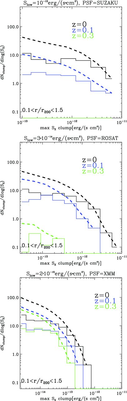
Average luminosity function of clumps detected in our sample of simulated X-ray maps at z = 0, z = 0.1 and z = 0.3. Each panel shows the estimate for a different assumed X-ray telescope (from top to bottom: Suzaku, ROSAT and XMM). The continuous lines are for the differential distribution, and the dashed lines are for the cumulative distributions.
Based on our results, a significant number of clumps can be detected in deep exposures with the three instruments: ∼20–30 per cluster with ROSAT/Suzaku, and ∼102 per cluster with XMM. These estimates are based on observations that sample the whole cluster atmosphere (1.2 × 1.2 R200). The evolution with redshift reduces the number of detectable clumps by ∼ 2–3, mainly due to the effect of the degrading spatial resolution with increasing distance (and not to significant cosmological evolution). At z = 0.3, only XMM observations would still detect some clumps (∼30 per cluster). The largest observable flux from clumps, based on these results, is ∼5 × 10⁻¹² erg (s cm−2) for Suzaku and ROSAT and ∼10−12 erg (s cm−2) for XMM.5
In the following we restrict ourselves to the fiducial case of z = 0.1 observations with XMM, and we study the statistical distributions of clumps in more detail.
In Fig. 7 we show differential distribution functions for the various parameters available for each detected clump: (a) maximum X-ray flux of each identified clump; (b) total X-ray flux on the pixel scale; (c) projected clump radius [assuming a full-width at half maximum (FWHM) of the distribution of SX6]; (d) projected distance from the cluster centre; (e) average projected temperature; (f) temperature contrast around the clump (estimated by dividing the temperature of the clump by the average surrounding temperature of the ICM, calculated as the average after the exclusion of the clump temperature).
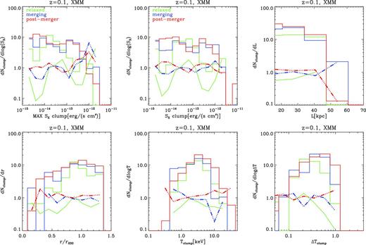
Differential distribution functions of clumps detected in our simulated X-ray maps at z = 0.1 and assuming SX, low = 2 × 10⁻¹⁵ erg (s cm−2) and an effective resolution of ≈10 arcsec (to mimic a deep survey with XMM). From left to right, we show: the distribution of the maximum and of the total flux of clumps and the distribution of FWHM in clumps in the top panels, the radial distribution, the temperature distribution and the distribution of temperature contrast of clump in the bottom panels. The different colours refer to the dynamical classes in which our sample is divided. All distributions have been normalized to the number of objects within each class. The lower dot–dashed lines show the ratio between clumps in the various dynamical classes, compared to the average population.
The luminosity distributions of clumps confirm the result of the previous section, and show that post-merger and merging clusters are characterized by a larger number of detectable clumps. They also host on average clumps with an approximately two to three times larger X-ray flux. Perturbed clusters have a factor of ∼2–4 excess of detectable clumps at all radii compared to relaxed clusters, and they host larger clumps. Clumps in post-merger systems are on average by a factor of ∼2 smaller than in merging systems, likely as an effect of stripping and disruption of clumps during the main merger phase. The distributions of temperatures and temperature contrasts show that the projected clumps are always colder than the surrounding ICM. This is because the innermost dense region of surviving clumps is shielded from the surrounding ICM, and retains its lower virial temperature for a few dynamical times (Tormen et al. 2003). For most of our detected clumps, the estimated FWHM is ≤50 kpc h−1. This is close to the cell size in our runs, and raises the problem that the innermost regions of our clumps are probably not yet converged with respect to resolution. We will revisit this issue again in the next section.
In Fig. 8, we investigate the dependence of the luminosity function of clumps on the projected radial distance from the centre (top panel) and on the total gas mass. We found that for all luminosity bins the intermediate annulus (0.6 ≤ R/R200 ≤ 1.2) contains >70 per cent of detectable clumps, even if its projected volume is about the same as that of the most external annulus. On the other hand, we detect no significant evolution with the host cluster mass. This is reasonable since we neglect radiative cooling or other processes than can break the self-similarity of our clusters.
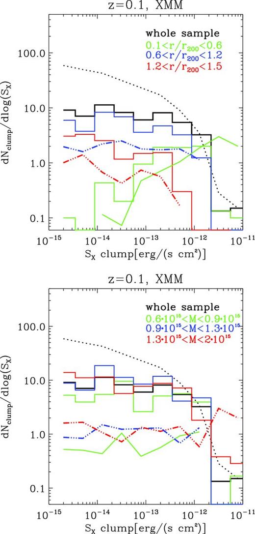
Different distribution functions of clumps detected in our simulated X-ray maps at z = 0.1 and assuming SX, low = 2 × 10⁻¹⁵ erg/(s cm−2) and an effective spatial resolution of ≈10 arcsec (to mimic a deep survey with XMM). The continuous lines are for the differential distribution, and the dashed lines are for the cumulative distributions (only the total is shown). The top panel shows the different luminosity functions for three different bins in the projected radii, and the bottom panel shows the decompositions of the data set into three total mass range. The dot–dashed lines show the ratio of objects found in each class, compared to the average population.
Given the relatively large number of detectable clumps predicted by our simulations, one may wonder whether existing observations with XMM, Suzaku, ROSAT or Chandra can already be compared with our results. We will come back to this point in Section 4.
3.3 Tests with additional physics and at higher resolution
Several physical and numerical effects may affect the amount of gas clumping factor measured in simulations. For instance, Nagai & Lau (2011) recently showed that the number of clumps in simulations with radiative cooling and feedback from supernovae and star formation is significantly larger than in non-radiative runs. However, clumps can cool so efficiently that they can eventually cool below X-ray emitting temperatures (Nagai & Lau 2011). Radiative cooling leads to the formation of more concentrated high-density clumps in the ICM, while feedback from SN and AGN may tend to wash them out by preventing the cooling catastrophe and providing the gas of clumps more thermal energy. The result of this competition between radiative losses and energy input via feedback may depend on the details of implementation. Also, the presence of CRs accelerated at cosmological shocks may yield a different compressibility of the ICM in the cluster outskirts, which can significantly change the amount of clumping there (Vazza et al. 2012).
In this section, we assess the uncertainty in our results, using a set of cluster re-simulations with different setups. Cluster runs such as the one we discussed in the previous sections are fairly expensive in terms of CPU time (∼3–4 × 10⁴ CPU hours for each cluster), given the number of high-resolution cells generated during the simulation. In order to monitor the effects of different setups we thus opted for a set of smaller clusters, already explored in Vazza (2011). We chose a pair of galaxy clusters with a final mass of ∼2–3 × 10¹⁴ M⊙ and two very different dynamical states (one post-merger and one relaxed cluster), and studied in detail the radial distribution of gas clumping factor in each of them. These clusters were re-simulated with the following numerical setups: (a) a simple non-radiative run, with a maximum resolution of 25 kpc h−1; (b) a run with pure radiative cooling, same peak resolution; (c) a run with thermal feedback from a single, central AGN starting at z = 1, with a power of Wjet ≈ 1044 erg s−1 for each injection, with the same peak resolution; (d) a run with a uniform pre-heating of 100 keVcm2 (released at z = 10) followed by a phase of thermal feedback from a central AGN starting at z = 1 and a power of Wjet ≈ 1043 erg s−1 for each injection; (e) a run with CR injection at shocks, reduced thermalization and pressure feedback, same peak resolution; (f) a simple non-radiative run at a higher resolution, 12 kpc h−1.
Cases (c) and (d) are taken from Vazza (2011), where we modelled the effects of a uniform pre-heating background of cosmic gas (following Younger & Bryan 2007) and of intermittent thermal AGN activity, modelled as bipolar outputs of overpressurized gas around the peak of cluster gas density. These runs were designed to fit the average thermal properties of nearby galaxy clusters (e.g. Cavagnolo et al. 2009) and to quench catastrophic cooling in radiative cluster simulations. We note that the amount of pre-heating and thermal energy release from the ‘AGN region’ was imposed by construction (in order to allow a parameter space exploration) and are not self-consistently derived from a run-time model of super-massive black holes evolution. In this implementation, we neglect star formation and therefore the energy feedback from supernovae and the gas mass drop-out term related to the star-forming phase is missing, leading to a higher baryon fraction of the hot gas phased compared to more self-consistent recipes (e.g. Borgani et al. 2008, and references therein). In our runs, the baryon fraction of the warm–hot medium is expected to be overestimated by a factor of ∼2 in the innermost cluster regions. Given that we excised the innermost 0.1R200 from the analysis of clumps of the previous section, this problem is not expected to be a major one.
Our model that includes CRs is taken from Vazza et al. (2012), and computes the run-time effects of diffusive shock acceleration (e.g. Kang & Jones 2007) in cosmological shocks: reduced thermalization efficiency at shock, injection of CRs energy characterized by the adiabatic index Γ = 4/3, pressure feedback on the thermal gas. This model was developed to perform run-time modifications of the dynamical effect of accelerated relativistic hadrons in large-scale structures. Given the acceleration efficiency of the assumed model (Kang & Jones 2007) the pressure ratio between CRs and gas is always small, ∼0.05–0.1 inside R200 of our simulated clusters at z = 0.
The feedback models discussed above are an idealized subset of feedback recipes that have been used by other authors (e.g. Cattaneo & Teyssier 2007; Sijacki et al. 2007; Gaspari et al. 2011). For the goal of this paper, they just represent extreme cases of dramatic cooling or of efficient heating in clusters, while the reality lies most likely in between.
Fig. 9 shows the projected X-ray maps and spectroscopic-like temperature maps for four re-simulations (a–b–d–f) for the merging cluster.
![Top panels: projected X-ray flux (log10LX [erg s−1]) of four resimulations of an ∼3 × 10¹⁴ M⊙ employing different physical implementations (see the main text for details). Bottom panels: projected spectroscopic-like temperature for the same runs (T in [K]).](https://oup.silverchair-cdn.com/oup/backfile/Content_public/Journal/mnras/429/1/10.1093/mnras/sts375/2/m_sts375fig9.jpeg?Expires=1750221962&Signature=1RJPUMvbwYEE6f27bEbiEQyHcw-pm7b6o8kJ1RL6bVzOqVotuIVTl0X70dtRvJ9vr7D1b2eDp9xH3deBbWitsAUSQ8tCPFizK8A7vKF56J-VjPvFL3hwQHeLfqbihiELSoZ9rNsYT0p5tGtLIfW4e9P4MymLwydcWNoPOwy4OtyxHgVf5tHZQXhy3cK4qpDc5njoYxw9VQr-0LUajar4GnQFfAEqky4W77Fr3KTscW4VBgrVhdgDpvFwqPfP4-GcggHnsM7G7MEBgEm9PyUgJco3F7UbrW4Cge6lA3fzWiBi6nsf3b62hLXAh9x98~AxV~yNVtM3SUIhgo5EFLYMbw__&Key-Pair-Id=APKAIE5G5CRDK6RD3PGA)
Top panels: projected X-ray flux (log10LX [erg s−1]) of four resimulations of an ∼3 × 10¹⁴ M⊙ employing different physical implementations (see the main text for details). Bottom panels: projected spectroscopic-like temperature for the same runs (T in [K]).
The corresponding profiles of average clumping factor and gas density for this cluster (bottom panels) and for the relaxed cluster (top panels) are shown in Fig. 10. The trend with the physical implementations is quite clear in both cases. The inclusion of cooling causes a ‘cooling catastrophe’ and the enhancement of the core gas density in both clusters. At the same time it also triggers the formation of denser and brighter clumps at all radii. A weak amount of thermal feedback from centrally located AGN is found to reduce the gas clumping factor only by a moderate amount, and only very close to the cluster centre (≤0.3R200), whereas it has no effect at larger radii. In these two runs the luminosity of the brightest clumps can be 10–102 times larger than in non-radiative runs. On the other hand, with a more efficient feedback recipe (early diffuse pre-heating a moderate AGN thermal feedback at low redshift) it seems possible to quench the cooling catastrophe in both clusters centre, and to reduce at the same time the gas clumping factor at all radii, making the latter only slightly larger than in the simple non-radiative run. The inclusion of CR feedback at cosmological shocks is found not to affect our gas clumping statistics compared to non-radiative runs. This can be explained because in our model the strongest dynamical effect of CRs is found around accretion shocks, where the energy ratio between injected CR energy and gas energy can be ∼10–20 per cent. However, filaments can enter far into the main cluster atmosphere avoiding strong accretion shocks, and thus keeping a smaller energy ratio of CRs. Given the strong role of filaments in enriching the ICM of clumpy material (as shown in Section 3.1), the fact that the overall clumping statistics within the cluster are not affected by the injection of CRs at shocks is not surprising.
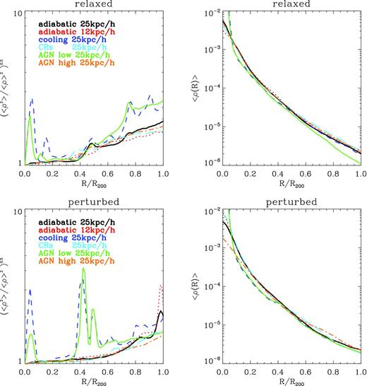
Left-hand panels: average profiles of clumping factor for a relaxed and a perturbed (i.e. with an ongoing merger) cluster in the mass range ∼2–3 × 10¹⁴ M⊙ resimulated with various physical recipes (plus one resimulation at higher resolution). Right-hand panels: gas density profiles for the corresponding runs on the left-hand panels.
Finally, we tested the effect of increasing spatial resolution on the gas clumping factor in our runs. On average, a larger resolution in the non-radiative runs is found not to change the overall gas clumping factor within the cluster, although assessing its effect on the high-density peaks of the clumps distribution is non-trivial. Indeed, the increase in resolution may change the ram-pressure stripping history of accreted clumps, causing a slightly different orbit of substructures towards the end of runs (e.g. Roediger & Brüggen 2007). This may lead to time-dependent features in the gas clumping factor profile, i.e. the higher resolution run of the perturbed cluster shows a ‘spike’ of enhanced clumping factor at ∼R200 at z = 0, while no such feature is detected in the resimulation of the relaxed system. The large-scale average trend of the gas clumping factor in both systems, instead, presents no systematic trend with resolution, suggesting that overall the effect of resolution in non-radiative runs is not significant for the spatial range explored here. However, we caution that some of the parameters of bright gas clumps derived in this work should be subject to some evolution with spatial resolution. The small number of clumps found in these two cluster runs is so small that we cannot perform meaningful clump statistics as in the previous section. However, we can already notice that the higher resolution increases the brightness of the clumps by a factor of ∼2–3. In addition, also the typical innermost radius of bright clumps can be only poorly constrained by our runs, and based on Section 3.2 our estimate of a typical ≤50 kpc h−1 must be considered as an upper limits of their real size, because the FWHM of most of our clumps is close to our maximum resolution, and this parameter has likely not yet converged with resolution.
In conclusion, the effect of radiative cooling has a dramatic impact on the properties of clumps in our simulations (as suggested by Nagai & Lau 2011). However, AGN feedback makes the X-ray flux from clumps very similar to the non-radiative case and the most important results of our analysis (Sections 3.1– 3.2) should hold. However, the trend with resolution is more difficult to estimate, given the large numerical cost of simulations at a much higher resolution. We therefore must defer the study of gas clumping statistics at much higher resolution to the future. This will also help to understand the number of unresolved gas clumps that might contribute to the X-ray emission of nearby clusters.
4 DISCUSSION AND CONCLUSIONS
In this paper we used a set of high-resolution cosmological simulations of massive galaxy clusters to explore the statistics and effects of overdense gas substructures in the intra-cluster medium. While the densest part of such gas substructures may be directly detected in X-ray against the smooth emission of the ICM, the moderate overdensity associated with substructure increases the gas clumping factor of the ICM, and may produce a (not resolved) contribution to the X-ray emission profiles of galaxy clusters.
We analysed the outputs of a sample of 20 massive systems (∼1015 M⊙) simulated at high resolution with the ENZO code (Norman et al. 2007; Collins et al. 2010). For each object we extracted the profile of the gas clumping factor within the full cluster volume, and within smaller volumes defined by projected sectors from the cluster centre. The gas clumping factor is found to increase with radius in all clusters, in agreement with Nagai & Lau (2011): it is consistent with 1 in the innermost cluster regions, and increases to |$C_(\rho ) \sim 3\hbox{--}5$| approaching the virial radius. Strongly perturbed systems (e.g. systems with an ongoing merger or post-merger systems) are on average characterized by a larger amount of gas clumping factor at all radii. This enhancement is associated with massive accretion of gas/DM along filaments, which also produces large-scale asymmetries in the radial profiles of clusters. Obtaining an accurate estimate of the enclosed baryon fraction for systems with large-scale accretions can be difficult because of the significant bias of gas clumping factor in the derivation of gas mass, and in the departure of real profiles from the NFW profile, which can bias the estimate of the underlying DM mass. In a realistic observation of a narrow sector from the centre of a cluster, the estimate of the enclosed baryon fraction can be biased by ±10 per cent in relaxed systems and by ±20 per cent in systems with large-scale asymmetries (not necessarily associated with major mergers).
In order to investigate the detectability of the high-density peaks of the distribution of gas clumping factor, we produced maps of X-ray emission in the [0.5-2] keV energy band for our clusters at different epochs. We extracted the gas clumps present in the images with a filtering technique, selecting all pixels brighter than twice the smoothed X-ray emission of the cluster. By compiling the luminosity functions and the distribution functions of the most important parameters of the clumps (such has their projected size, temperature and temperature contrast with the surrounding ICM) we studied the evolution of these distributions as a function of the mass and of the dynamical state of the host cluster, and of the epoch of observation. Summarizing our results on clumps statistics, we find that (a) there is a significant dependence on the number of bright clumps and the dynamical state of the host cluster, with the most perturbed systems hosting on average a factor of ∼2–10 more clumps at all radii and luminosities, compared to the most relaxed systems; (b) the host cluster mass, on the other hand, does not affect the number of bright clumps (although the investigated mass range is not large; ∼0.3 dex); (c) about a half of detectable bright clumps are located in the radial range 0.6 ≤ R/R200 ≤ 1.2 from the projected cluster centre, while a very small amount of clumps per cluster (order 1) are located inside <0.6R/R200 ; (d) the typical size of most of gas clumps (extrapolated by our data) is ≤50 kpc h−1. In a preliminary analysis based on a few re-simulations of two simulated clusters with different recipes of CR physics or AGN feedback, we tested the stability of our results with respect to complex physical models. Radiative cooling dramatically increases the observable amount of gas clumping (Nagai & Lau 2011). However, the required energy release from AGN seems to be able to limit at the same time the cooling flow catastrophe, and the observed clumping factor down to the statistics of simpler non-radiative estimates. The increase of resolution does not significantly change the observed number of detectable clumps or the gas clumping factor of the ICM. However, resimulations at higher resolution produce a ∼2–3 larger maximum X-ray flux in the clumps, and therefore in order to assess the numerical convergence on this parameter further investigations are likely to be necessary. Also the typical size of bright clumps cannot yet be robustly constrained by our data, which only allow us to place an upper limit of the order of ≤50 kpc h−1.
We conclude by noting that based on our results of the statistics of bright clumps (Section 3.2) it seems likely that a given number of them could already be present in existing X-ray observations by XMM and by ROSAT (and, to a much lesser extent given the expected lower statistics, by Suzaku). However, it is very difficult to distinguish bright gas clumps from more point-like sources (like galaxies or AGN), given that their expected size is very small (<50 kpc h−1), typically close to the effective PSF of instruments. In a real observation, a catalogue of point-like sources is generated during the data reduction, and excised from the image.
In order to perform a first check of the our quantitative results, we examined the catalogue of point-sources generated in a real ROSAT observations of Eckert et al. (2012). In Fig. 11 we show the luminosity and the radial distribution of point-like sources from the ROSAT observation of A2142, and the corresponding simulated statistics obtained by analysing the whole simulated data set at the same resolution and flux threshold of the real observation. The luminosity distributions are taken for two radial bins: 0.1 ≤ R/R200 < 0.6 and 0.6 ≤ R/R200 < 1.2.
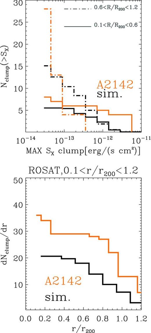
Top panel: cumulative distribution of luminosity of simulated clumps (in black; the average over the whole data set is considered) and of point-like sources in the ROSAT observation of A2142 (in orange, taken from Eckert et al. 2012). The solid lines show the distributions inside 0.1 ≤ R/R200 < 0.6; the dot–dashed lines show the distribution inside 0.6 ≤ R/R200 < 1.2. Bottom panel: cumulative radial distribution of simulated clumps and point-like sources for the same data sets.
The number of point-like sources in the real observation is ∼1.5–2 times larger than the simulated distribution of clumps at all radii. The observed luminosity distribution inside the innermost radial bin also shows an excess with respect to the simulated clumps at all luminosities. In the outer bin, however, the observed luminosity distribution has a totally different shape with respect to the simulated one. It should be noticed that in the outer regions the sensitivity to point-like sources in the real observation is much degraded. Therefore, it appears likely that the change in the observed luminosity distribution function of point-like sources is mainly driven by instrumental effects. We found very similar results in the catalogue of point-sources of the ROSAT observation of PK 0754−191 of Eckert et al. (2012). Based on such small statistics, and given the degrading sensitivity of ROSAT to point-like sources at large radii, it is still premature to derive stronger conclusions. The number of expected point-like sources brighter than ∼3 × 10⁻¹⁴ erg (s cm−2) in the field is ∼20 deg−2, based on the collection of wide field and deep pencil surveys performed with ROSAT, Chandra and XMM by Moretti et al. (2003). Given the projected area of the A2142 observation of Eckert et al. (2012), the expected number of point-like field sources is ∼6–8 inside R200, significantly smaller than both the point-like sources detected in the field of A2142 and the total number of simulated clumps (that are of the order of ∼40 within R200). However, one should note that the density of galaxies in a cluster field is much higher than in a typical field, and so is the number of AGNs (see e.g. Martini, Mulchaey & Kelson 2007; Haines et al. 2012). Thus, the larger number of detected point sources compared to the expectation from background AGN cannot be directly used as evidence for gas clumping.
It is possible that a significant fraction of such point-like sources are compact and bright self-gravitating gas clumps in clusters. However, it is unlikely that they can be identified based on their X-ray morphology, given their small size. In the case of high-resolution Chandra images of nearby clusters, it is possible that some existing data can actually contain indications of gas clumps. Their detection, however, is made complex by the strong luminosity contrast required for them to be detected against the bright innermost cluster atmosphere. Very recently, the application of sophisticated analysis techniques has indeed suggested that some gas clumps (with size ≤100–200 kpc) may actually be present in nearby Chandra observations (Andrade-Santos, Lima Neto & Laganá 2012).
In the near future, cross-correlating with the additional information of temperature in case of available X-ray spectra may unveil the presence of gas clumps in the X-ray images (Fig. 7).
We thank our referee for useful comments that greatly improved the quality of our manuscript. FV and MB acknowledge support through grant FOR1254 from the Deutsche Forschungsgemeinschaft (DFG). FV acknowledges computational resources under the CINECA-INAF 2008-2010 agreement. SE and FV acknowledge the financial contribution from contracts ASI-INAF I/023/05/0 and I/088/06/0. We acknowledge G. Brunetti and C. Gheller for fruitful collaboration in the production of the simulation runs. Support for this work was provided to AS by NASA through Einstein Postdoctoral Fellowship grant number PF9-00070 awarded by the Chandra X-ray Center, which is operated by the Smithsonian Astrophysical Observatory for NASA under contract NAS8-03060. We thank Marc Audard for kindly providing us his code for the X-ray cooling function.
While this article was under review, Zhuravleva et al. (2012) published a work in which they also characterize the level of inhomogeneities in the simulated ICM, based on the radial median value of gas density and pressure. They study the impact of cluster triaxiality and gas clumping in the derivation of global cluster properties such like the gas mass and the gas mass fraction, reporting conclusions in qualitative agreement with our work.
We checked that the use of the DM overdensity statistics, in this case, yields very similar results to those obtained using the gas overdensity. However, we focus on the latter in this work, since this quantity can be more easily related to observations.
More exactly, we adopted z = 0.023, corresponding to the luminosity distance of the COMA cluster, ≈100 Mpc.
We note that the maximum observable flux here is not completely an intrinsic property of the clumps, but it also slightly depends on the post-processing extraction of clumps in the projected maps at different resolution, as in Section 2.2.1. For large PSF, indeed, the blending of close clumps can produce a boost in the detectable X-ray flux within the PSF.
The projected clump radius is measured here with an extrapolation by assuming that the observed flux from clumps originates from a Gaussian distribution, for which we compute the FWHM. This choice is motivated by the fact that in most cases our detected clumps are very close to the resolution limit of our mock observations, and only with some extrapolation we can avoid too coarse a binning of these data. For this reason, our measure of the clump radius must be considered only a first order estimate, for which higher resolution is required in order to achieve a better accuracy.
