


Abstract
Since 2011 February 27 a new differential image motion monitor (DIMM) has been operating at Roque de los Muchachos Observatory close to the Telescopio Nazionale Galileo (TNG). The purpose of this instrument is to provide useful information about the optical turbulence for astronomical observations in the neighbourhood of the TNG. We present the first statistical results from it as well as, for the first time, the relationship between the principal components analysis of local-ground atmospheric parameters and seeing. We focus on the possibility of reliable predictions concerning the future behaviour of the seeing.
1 INTRODUCTION
The seeing is one of the most important parameters in determining the site quality of astronomical observatories. Most professional observatories have measured this parameter during long-term campaigns, and some of them also have permanent measurement programs. This is the case for the Roque de los Muchachos Observatory (La Palma) through the Sky Quality Group of the Instituto de Astrofísica de Canarias (IAC; Muñoz-Tuñón, Vernin & Varela 1997) and the Isaac Newton Group (ING).1
Various techniques have been used to measure the atmospheric turbulence: during 1989–1990 the Differential Image Motion Monitor (DIMM; Sarazin & Roddier 1990) was introduced, which became the standard instrument for measuring the seeing. DIMM has been established as the most widely used instrument for conducting intensive, extensive, multi-site site-testing campaigns to select the best location to host the next generation of telescopes such as the Thirty Meters Telescope (TMT) and the Extremely Large Telescope (ELT).
The basis of the DIMM technique is explained in many articles (Martin 1987; Sarazin & Roddier 1990; Vernin & Muñoz-Tuñón 1995; Tokovinin 2002), and it is now used regularly in observatories around the world. Throughout 2009 and 2010, a semi-automatic and remote-use DIMM (hereafter DIMM@TNG) was built at the Telescopio Nazionale Galileo (TNG). In this paper we present the instrument, the first statistical results and a preliminary analysis based on the principal component analysis (PCA) of various atmospheric parameters. The main advantage of the PCA is the capability to manage each variable as independent.
2 INSTRUMENTATION AND DATA
2.1 An overview of DIMM@TNG
It is difficult to separate the variance induced by the turbulence from that induced by the telescope, as the telescope is not rigid: images are, in fact, affected by bad tracking, guide defects, mechanical stress, wind gusts, effects due to the dome, and so on. So, extra terms should be added to the variance of the position of images. Consequently, the DIMM method makes use of a differential procedure instead of the absolute motion of the image (Martin 1987; Sarazin & Roddier 1990; Vernin & Muñoz-Tuñón 1995; Tokovinin 2002). DIMM consists of two pupils of the same size on a common mount; a prism on one of the pupils allows a well-separated double image to form on the focal plane. The image motion induced by the telescope is removed by taking account of the difference of the positions of the images produced by each pupil. This does not remove the changes induced by turbulence, as it is slightly different for each pupil: the wavefront is wrinkled by atmospheric turbulence and the angle of arrival (or tilt) of the wavefront is not uniform.
Variance is calculated after 300 frames with an exposure time of 10 ms, with two notable exceptions according to the magnitude of the star observed (Alpheratz m = 2.2 with an exposure time of 15 ms and Arcturus m = −0.04 with 5 ms), and corrected for the cosine of the zenith distance. A seeing value is returned approximately every 51 s. DIMM is sensitive to atmospheric fluctuations only on scales comparable to the distance between the two pupils. These high-frequency fluctuations are missed if the turbulent layer moves appreciably during the single frames, and the variance of the positions is underestimated. Because DIMM@TNG does not correct this effect, called the exposure-time bias, it delivers a seeing that is smaller than the real value when the wind speed at some turbulent layer is greater than ∼15 m s−1.
Because the FWHM varies as the 6/5 power of the standard deviation of the motion, an error in the determination of the pixel scale produces a 6/5 times larger error in the final FWHM. For this reason, the pixel scale is regularly checked by imaging with optical double stars of known separation. In fact, the pixel size is determined with an accuracy of ∼1 per cent.
The DIMM@TNG also measures the scintillation index σ2I, strongly related to the isoplanatic angle, as the flux variance normalized by the square of the mean flux measured with an 80-mm aperture.
2.2 Defocus tolerance
In our DIMM, we have 0.5 rad of Zernike defocus for rc ≈ 6300 m. The deviation of DIMM spots from their optimal difference (45 pixels) owing to the defocus is equal to the derivative of l over r; that is, to d/rc. In our case we obtain 6.5 arcsec, which is equivalent to 15 pixels. For these reasons we have the assurance that when the distance between the spots is within 45 ± 15 pixels, then the defocus is not greater than 0.5 rad.
2.3 Sources of error
2.3.1 Dark-frame noise
In our case the CCD detector is a Sony ICX098AL/BL with an ADC resolution/output of 8 bit, showing counts between 0 and 255. Under standard imaging conditions (luminance: 706 cd m−2, colour temperature of 3200K, halogen source) various characteristics of the detector have been measured, giving the following results: peak quantum efficiency = 55 per cent at λ = 460 nm, saturation signal = 550 mV, charge capacity = 20 000 e−, output sensitivity = 27.5 μV/e−, readout noise = 20 e−, dark signal (measured as the average value of the signal output and the device in the light-obstructed state) = 4 mV, and dark signal shading (measured as the interval between the maximum and minimum values of the dark signal output) = 1 mV.
Moreover, we examined the typical dark frame of our CCD at a temperature of 25°C with an exposure time of 10 ms. As shown in Table 2, over 95 per cent of the pixels have zero counts and only 0.17 per cent have two or more counts. For this reason we consider the noise contribution of the dark frame as negligible.
2.3.2 Noise variance
In our case, we have adjusted the window size to the first Airy disc of the pupil entrance or slightly larger (10 pixels), and the typical noise is σ2ins = 0.008 ± 0.002 arcsec. This is a very low value that we left uncorrected.
We also analysed the optical quality of images obtained with Strehl ratios between 0.3 and 0.45.
2.3.3 Statistical errors
Thus it is the main source of uncertainty in the final result of seeing.
2.4 Location
The instrument is on a tower 5 m in height in order to avoid any contribution from the ground layer. The tower is along the external north face of the Caldera de Taburiente, 125 m southwest of TNG and 400 m south-southeast of the Gran Telescopio de Canarias (GTC), as shown in Fig. 1. This location was thoroughly studied by the IAC two decades ago (Muñoz-Tuñón et al. 1997) and was named Site A.
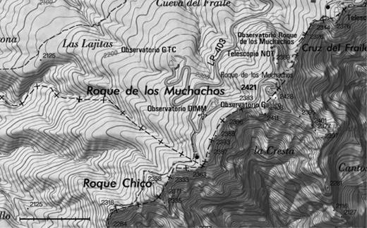
Location of the DIMM@TNG. The instrument is located at the centre of the image (white cross) and is labelled ‘Observatorio DIMM’. The double-black lines are the asphalted access roads to the telescopes, and the light-grey ones are the altitude contour lines. The bar in the lower-left corner represents 500 m and is divided into five fractions of 100 m each.
2.5 Seeing measurements
In this analysis we chose a period of time of 10 months (from 2011 May to 2012 February), during which DIMM@TNG carried out 106 858 seeing measurements over 209 nights of observations. First, from the raw data base, we rejected 6040 records. Some of them did not contain measurements (probably as a result of communication error between telescope and data base). Others did not have the right seeing values owing to a measurement failure: the variance is calculated using 300 consecutive frames, but in some of the series, especially when the sky is covered with cirrus and clouds, there are a few frames in which the flux of the star images is insufficient to enable correct measurement of their barycentre, distorting the final seeing result. This problem was recently solved by implementing a filter to discard images.
We then excluded another 15 870 measurements that are outside the defocus tolerance or for which the difference between parallel and perpendicular seeing is greater than 20 per cent. Fig. 2 shows the two constraints as dashed lines: the points with valid values of seeing are in the dashed rectangle. After these checks, the valid data sample that we used had 84 436 seeing measurements.
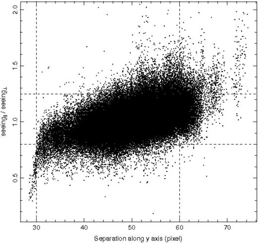
y separation of star images versus parallel to perpendicular seeing. The dashed lines show the constraints for the valid data (see text).
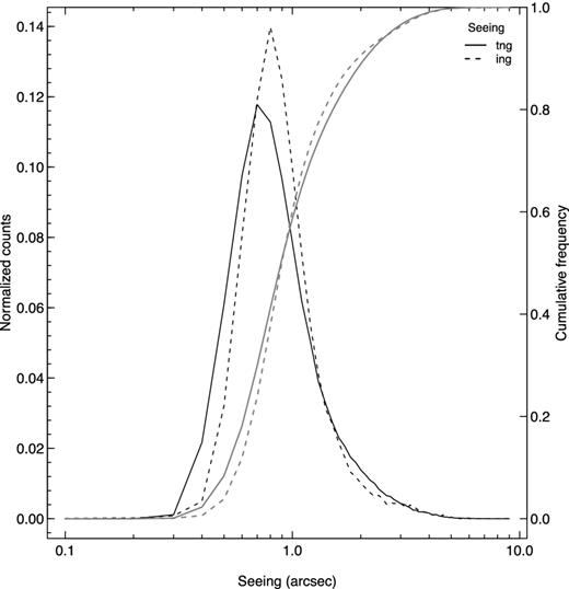
Distributions of the whole valid data sample of DIMM@TNG (dark-solid line) and original data of RoboDIMM (dark-dashed line) from 2011 May to 2012 February. The grey lines represent the cumulative distributions (right y-axis) with the same significance of the symbols.
Table 3 shows a statistical summary of the observations during the considered period. Each row shows the number of observing nights, number of seeing measurements, 25th percentile, mean, and 75th percentile of seeing calculated every month.
The mean and median seeing values of the whole period are 0.96 and 0.89 arcsec, respectively (see also the plot in Fig. 3, dark-solid line). The minimum monthly median seeing is 0.70 arcsec, obtained in 2011 August (the month of September has too few measurements); the worst month is 2011 December, with a median seeing of 1.26 arcsec. Figs 4 and 5 show the weekly distributions of seeing and scintillation index, respectively.
3 COMPARATIVE MEASUREMENTS
3.1 DIMM@TNG versus LRS@TNG
In order to verify the correct operation of the DIMM@TNG, we performed a comparison between its measurements and the values obtained using images taken with DOLORES (Device Optimized for LOw RESolution, hereafter LRS@TNG). For this purpose, on the night of 2010 August 5 the DIMM telescope was installed inside the TNG dome to measure the seeing in environmental conditions most similar to those in TNG.
A procedure similar to this was also used in Sarazin & Roddier (1990) to compare the ESO-DIMM with the images taken by a 2.2-m telescope in La Silla in order to verify the proper operation of the DIMM. The good results obtained on that occasion were the main incentive to carry out the same experimental validation of our DIMM, in spite of the objections that can be made because the DIMM is an instrument insensitive to the outer scale while a 3.5-m telescope diameter is sensitive to this parameter. It should be noted here that what we are really comparing is the seeing measured by the DIMM with the image quality obtained through a telescope (see Section 2.1). Only in the case where the outer scale (10–100 m) (Ziad 2000) is clearly greater than the diameter of the telescope is the point spread function of the telescope images not severely affected by the factor L0.
Because TNG is installed on an alt–az mount and the DIMM@TNG on an equatorial mount, we were necessarily limited to pointing the telescope at a field in the sky where the azimuth movement was minimal, as close to the pole as possible. We chose an arbitrary field where LRS@TNG with the filter V Johnson detects enough stars to obtain usable seeing measurements with an exposure time of 40 s and where the autoguide of the telescope behaves stably (α = 12h00m00s and δ = 89°20′00′′). In this position the only star compatible with the constraints of a standard DIMM (stars of less than 2 mag) is αUMi (V = 1.97).
To avoid as far as possible any deterioration of the image quality in LRS@TNG, we used the active optics system of TNG. Then, we proceeded to conduct a Shack–Hartmann analysis to remove static aberrations in the optics of the telescope when we point at such a low elevation, namely ∼28°. We chose a star near to the pole, HIP3128 (α = 00h39m42|$.\!\!^{ {\mathrm{s}}}$|6 and δ = 89°26′39| ${.\!\!\!\!\!\!^{\prime\prime}}$|5, V = 8.10), to do an analysis of the aberrations, and after the active optics correction we obtained a concentration of 80 per cent of the energy in 0.12 arcsec.
Once the active optics correction was made, we pointed to the chosen field and focused. We then proceeded to point the DIMM@TNG to αUMi in order to take measurements that were uninterrupted and quasi-simultaneous with images taken with LRS@TNG in band V. During the night, 548 measurements of seeing were taken with the DIMM@TNG at a rate of one measurement every 51 s, and 404 images were taken with LRS@TNG at a rate of one per minute (40 s of exposure and 20 s of reading).
In the images taken with LRS@TNG, we applied a bias correction with iraf2 and used a program written in idl to proceed to measure the FWHM of five stars distributed over the entire CCD field. FWHM measurements were made along the x- and y-axes for each star, and with a scale plate in CCD LRS@TNG (0.252 arcsec pixel−1) it was possible to obtain values of seeing split into two components. The seeing values considered for this analysis are the mean averages of the components x and y.
The high value of the correlation coefficient and the peak of the distribution of the difference between the measurements near to zero (Fig. 6d) indicate that the two instruments are in good accordance.
3.2 DIMM@TNG versus RoboDIMM
RoboDIMM of the ING is the only DIMM that operated on the Observatorio del Roque de los Muchachos (ORM) during the period of our analysis. The data are public and available on the ING web pages.3 RoboDIMM is 1100 m north-east of DIMM@TNG, and nearly 50 m lower. The telescope aperture has a mask with four pupils and takes four seeing measurements (two parallel and two perpendicular) every 3 min.
The seeing values used for the comparison are the averages of the perpendicular and parallel measurements made by the respective telescope; we used original data for RoboDIMM, and our valid data sample (see Section 2.5) for DIMM@TNG.
Despite the differences between the two instruments (i.e. geographic location, work procedure and amount of data sampled), values in Table 4 show that the two seeing distributions are comparable: mean and median differences are only 0.1 and 0.08 arcsec, respectively, with RoboDIMM values slightly higher.
DIMM@TNG technical parameters.
| DIMM@TNG | |
|---|---|
| Telescope | Celestron CGE1100 (XLT) |
| Focal | 2800 mm |
| f-ratio | f/10 |
| Pupil diameter | 80 mm |
| Pupil separation | 198 mm |
| Prism angle wedge | 40 arcsec |
| CCD detector | Sony ICX098AL/BL |
| CCD format | 640 × 480 pixel |
| Pixel size | 5.62 × 5.62 μm |
| FOV | 4.62 × 3.52 arcmin |
| Plate scale | 0.432 ± 0.004 arcsec pixel−1 |
Typical CCD dark frame at T = 25°C and an exposure time of 10 ms.
| Count | Number of pixels | Per cent | Cumulative per cent |
|---|---|---|---|
| 0 | 292285 | 95.14 | 95.14 |
| 1 | 14387 | 4.68 | 99.83 |
| 2 | 309 | 0.10 | 99.93 |
| 3 | 117 | 0.04 | 99.97 |
| 4 | 59 | 0.02 | 99.99 |
| 5 | 43 | 0.01 | 100.00 |
| Count | Number of pixels | Per cent | Cumulative per cent |
|---|---|---|---|
| 0 | 292285 | 95.14 | 95.14 |
| 1 | 14387 | 4.68 | 99.83 |
| 2 | 309 | 0.10 | 99.93 |
| 3 | 117 | 0.04 | 99.97 |
| 4 | 59 | 0.02 | 99.99 |
| 5 | 43 | 0.01 | 100.00 |
Monthly statistics of seeing measured by DIMM@TNG during the period from 2011 May to 2012 February.
| Month | Night | Data | 1st quartile | Median | 3rd quartile |
|---|---|---|---|---|---|
| (arcsec) | (arcsec) | (arcsec) | |||
| 05-11 | 14 | 6061 | 0.62 | 0.75 | 1.00 |
| 06-11 | 17 | 5513 | 0.64 | 0.89 | 1.35 |
| 07-11 | 25 | 8895 | 0.71 | 1.01 | 1.62 |
| 08-11 | 31 | 10977 | 0.52 | 0.70 | 0.96 |
| 09-11 | 4 | 2151 | 0.56 | 0.70 | 0.89 |
| 10-11 | 16 | 6191 | 0.70 | 0.88 | 1.16 |
| 11-11 | 22 | 8965 | 0.66 | 0.83 | 1.08 |
| 12-11 | 29 | 11947 | 0.86 | 1.26 | 1.76 |
| 01-12 | 30 | 16039 | 0.61 | 0.84 | 1.25 |
| 02-12 | 21 | 7697 | 0.83 | 1.15 | 2.03 |
| Total | 209 | 84436 | 0.65 | 0.89 | 1.31 |
Comparison between seeing distributions of DIMM@TNG and RoboDIMM when the two telescopes worked at the same time. As for Table 3, the mean and interval limits were calculated using logarithmic seeing values.
| Telescope | Mean | Median |
|---|---|---|
| (arcsec) | (arcsec) | |
| DIMM@TNG | 0.93+ 1.52− 0.57 | 0.86 |
| RoboDIMM | 1.03+ 1.68− 0.63 | 0.94 |
| Telescope | Mean | Median |
|---|---|---|
| (arcsec) | (arcsec) | |
| DIMM@TNG | 0.93+ 1.52− 0.57 | 0.86 |
| RoboDIMM | 1.03+ 1.68− 0.63 | 0.94 |
4 THE PRINCIPAL COMPONENT ANALYSIS
In this section we investigate the environmental conditions that produce a given value of seeing using the collection of meteorological data recorded by the TNG weather station. These conditions are the main determinant of image quality.
The station was installed in 1998 on a 15-m-high tower, 30 m from the position of DIMM@TNG (Porceddu et al. 2002). Every 30 s the station measures several atmospheric variables: air temperature at various levels above the ground, namely 2 m (T2), 5 m (T5) and 10 m (T10), relative humidity (RH), and atmospheric pressure (P). A full description of the station, the type of sensors, and their accuracy is given in Porceddu et al. (2002).
Thanks to the presence of temperature sensors at different levels, we could add three further variables to check the stratification and stability of the local atmospheric layers. We defined ΔTa, b, with a, b ∈ {2, 5, 10} and a > b, as the temperature gradient calculated between the air-temperature sensors at levels a and b.
To compare these eight atmospheric variables with seeing measurements of the DIMM@TNG, we extracted a night subsample and calculated the mean value of each minute for a period of one year starting on 2011 March 1. To have a homogeneous sample of data, we rejected each minute data set if one of the sensor data points was not available. After this operation, the final sample comprised m = 251 389 measurements for each variable. Some statistics are presented in Table 5.
On account of the high number of data involved, both seeing and atmospheric-variable measurements, we decided to use a statistical tool to extract the most interesting information from the atmospheric variables and successively to compare them with the seeing. We decided on principal component analysis (PCA), which is a multivariate statistic that uses orthogonal transformations to convert a data sample (in our case atmospheric variables) into a set of linearly uncorrelated variables (the principal components).
The new orthogonal basis is calculated to maximize the variance of the projection between the two coordinate systems, so that the first coordinate (i.e. the first principal component) has the greatest variance of the projections, the second has the next greatest variance, and so on. In this manner the first principal component contains most of the information of the true variables and highlights their variation.
The calculation of eigenvalues and eigenvectors is subject to a sampling error (see equation 24 of North et al. 1982 and equation 9 of Quadrelli, Bretherton, Wallace 2005), but, owing to the large number of data considered here (thousands), this source of error can be considered negligible.
The principal components were calculated using one-year nightly data of P, RH, one air temperature (T10) and one temperature gradient (ΔT10, 5); prior to this, the data had been scaled by means and normalized by standard deviations of their own distribution using the values listed in rows three and four of Table 5. Correlated variables (highlighted in bold in Table 6) were rejected to avoid unuseful (or marginally useful) data. The sampling errors of eigenvalues and eigenvectores are all of the order of magnitude of 103.
We focused our analysis on the first principal component (PC1), which explains 55 per cent of the variation of the variables (see Table 7). As shown in Table 7, PC1 takes account especially of temperature and pressure (the two coefficients have almost similar values). In this analysis we expected to find a clear dependence of the seeing with respect to at least one of the principal components, but with the set of data currently available we did not see any kind of signal in this direction. We hope, with longer time series, to obtain better results. The analysis of the distribution of PC1, discussed in Section 5, seems to be more promising.
5 DISCUSSION
The first 10-month collection of data from the new DIMM@TNG allowed us to make some preliminary analysis of the reliability of the data itself and a comparison with various atmospheric variables.
The monthly distribution of the seeing (see solid circles and lines in Fig. 7, and Table 3) shows a weak seasonal trend, which is clearer in the longer data sample of RoboDIMM (white diamonds and dashed lines of Fig. 7), for which we used three years of data (2009, 2010, 2011). In general, seeing measurements are better during warm months (i.e. from May to September) than in the remaining period. At this stage the result is encouraging: we expect that with more measurements our data will show a similar distribution.
Main statistics of atmospheric variables recorded by the TNG weather station during the period between 2011 March 1 and 2012 March 2.
| T2 | T5 | T10 | RH | P | ΔT10, 2 | ΔT5, 2 | ΔT10, 5 | |
|---|---|---|---|---|---|---|---|---|
| (°C) | (°C) | (°C) | (per cent) | (hPa) | (°C) | (°C) | (°C) | |
| Min | −6.8 | −6.6 | −6.7 | 3 | 754.6 | −4.0 | −1.0 | −4.2 |
| Max | 22.1 | 22.4 | 22.5 | 100 | 779.2 | 3.4 | 3.2 | 2.7 |
| Mean | 8.0 | 8.3 | 8.4 | 35 | 771.5 | 0.4 | 0.3 | 0.1 |
| Std dev. | 5.5 | 5.5 | 5.5 | 30 | 4.1 | 0.5 | 0.3 | 0.3 |
Correlation matrix of the atmospheric variables. Bold denotes strong and weak correlations cited in the text.
| T2 | T5 | T10 | RH | P | ΔT10, 2 | ΔT5, 2 | ΔT10, 5 | |
|---|---|---|---|---|---|---|---|---|
| T2 | 1.000 | |||||||
| T5 | 0.999 | 1.000 | ||||||
| T10 | 0.997 | 0.999 | 1.000 | |||||
| RH | −0.495 | −0.510 | −0.516 | 1.000 | ||||
| P | 0.645 | 0.646 | 0.651 | −0.520 | 1.000 | |||
| ΔT10, 2 | 0.155 | 0.198 | 0.235 | −0.344 | 0.191 | 1.000 | ||
| ΔT5, 2 | 0.146 | 0.199 | 0.209 | −0.346 | 0.119 | 0.796 | 1.000 | |
| ΔT10, 5 | 0.092 | 0.103 | 0.153 | −0.181 | 0.178 | 0.752 | 0.213 | 1.000 |
Results of the principal component analysis: the first three lines are the importance of the components; the others are the coefficients of the linear transformation between the two sets of variables. Bold values highlight the most important coefficients of the PCs.
| PC1 | PC2 | PC3 | PC4 | |
|---|---|---|---|---|
| Standard deviation | 1.483 ± 0.006 | 0.964 ± 0.003 | 0.723 ± 0.001 | 0.591 ± 0.001 |
| Proportion of variance | 0.550 | 0.232 | 0.131 | 0.087 |
| Cumulative proportion | 0.550 | 0.782 | 0.913 | 1.000 |
| T10 | 0.572 ± 0.002 | −0.184 ± 0.001 | 0.383 ± 0.002 | − 0.701 ± 0.003 |
| ΔT10, 5 | 0.239 ± 0.002 | 0.969 ± 0.001 | 0.058 ± 0.003 | −0.028 ± 0.002 |
| RH | −0.532 ± 0.001 | 0.081 ± 0.002 | 0.843 ± 0.001 | 0.005 ± 0.005 |
| P | 0.577 ± 0.001 | −0.143 ± 0.001 | 0.373 ± 0.002 | 0.712 ± 0.003 |
For instance , the difference between the values of June and July is probably caused by short-time fluctuations of atmospheric variables that occurred in some period of 2011. We note that, excluding the nights of 2011 June 13 and 24 from the statistical computation, the monthly mean and median of 2011 June were similar to the values obtained with the 3-yr data of RoboDIMM: 0.88 and 0.83, respectively. We are not surprised that, comparing the monthly mean of wind speed of June and July from 2009 to 2011, the values obtained in 2011 are the highest: 6.0 (2009), 5.8 (2010) and 7.0 m s−1 (2011) for June, and 5.4 (2009), 5.5 (2010) and 6.9 m s−1 (2011) for July.
A short-period analysis made using weekly means (shown in Fig. 4) does not reveal any particular trend, with a succession of good (e.g. the weeks from 2011 August 21 to 2011 September 4) and bad (e.g. the weeks from 2011 December 24 to 2012 January 21) seeing periods, with some exceptions.
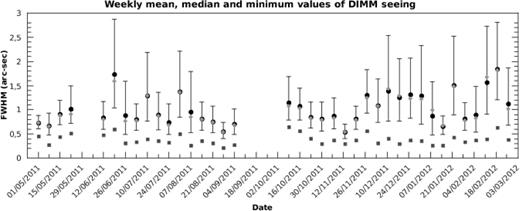
Weekly summaries of DIMM@TNG seeing data. The dark-grey squares are the minimum seeing values of the week; the light-grey diamonds are the medians; the black circles are the mean values deduced from logarithmic means. The error bars correspond to ±1σ of the lognormal weekly distribution.
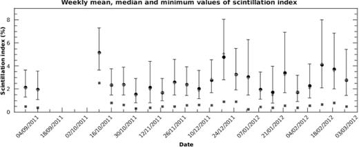
Weekly summaries of scintillation index data taken with the DIMM@TNG. The dark-grey squares are the minimum scintillation index values of the week; the light-grey diamonds are the medians; the black dots are the mean values deduced from logarithmic means. The error bars correspond to ±1σ of the lognormal weekly distribution.
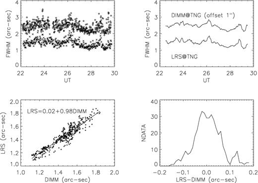
(a) The seeing data measured by LRS@TNG (crosses) and DIMM@TNG with an offset of 1 arcsec (diamonds). (b) The same data smoothed. (c) The best-fitting and the linear regression. (d) The distribution of the difference between the data.
The PCA is more promising – a previous study using PCA with atmospheric variables and seeing was made by de Gurtubai et al. (2002). In that work, data from 90 nights of observations were used, and PCA was calculated using atmospheric variables and seeing. In this work we tried a different approach, calculating principal components using only atmospheric variables to compare them with seeing.
As in the work of de Gurtubai et al. (2002), a direct comparison of principal components with the seeing is not significant, but PC1 shows a bimodal-normal distribution (see the white histogram in Fig. 8), with the main peak about five time higher than the secondary.
PC1, in fact, is influenced by seasonal atmospheric conditions, especially temperature and pressure (see Section 4): the main peak, at PC1 = 0.2, is an expression of more stable weather conditions than at the secondary one (PC1 = −3.6), where temperature and pressure are lower. This kind of distribution suggests that the variation between the two conditions is not linear, but temperature and pressure seem to change quickly from one configuration to another. The analysis of the monthly distribution of PC1 compared with seeing (solid lines in Fig. 9) revealed that the months with a bimodal distribution are February, March and April; these months provide almost the whole contribution to the secondary peak. The distribution in November also shows two peaks, but the secondary one is at PC1 = −2.4, between the other two peaks located in PC1=0.2 and PC1=−3.6.
The measurements of atmospheric variables taken at the same time as seeing measurements of DIMM@TNG are 28 per cent of the total (see the grey histogram in Fig. 8 for comparison). Usually this difference would arise mainly as a result of adverse weather conditions (cloud, wind speed >15 m s−1, RH > 85 per cent), but, in this first period of operation of DIMM@TNG, it could also be caused by technical issues. However, it can be noted that seeing measurements are possible in most cases when PC1 is near the main peak of the whole distribution: only a few seeing values (less than 1 per cent, most of them taken in 2012 February) are observed with PC1 <−2.
6 CONCLUSION
In this work we have presented the first statistical data analysis of the new DIMM working at Roque de los Muchachos Observatory, close to TNG.
The first 10 months of measurements (from 2011 May to 2012 February) were analysed to exclude bias and systematic errors and to reject values that did not respect the constraints of the system (i.e. parallel and perpendicular seeing ratio and defocus tolerance). The valid data sample contains more than 80 000 measurements.
The mean and median seeing values of this first 10 months of working are 0.96 and 0.89 arcsec, respectively. The monthly statistic (shown in Table 3) indicates a weak seasonal trend of the seeing.
The seeing values of DIMM@TNG were compared with the FWHM measured by LRS@TNG during the night of 2010 August 5. The measurements were made under environmental conditions as similar as possible to those in TNG, moving the telescope of the DIMM inside the dome of TNG. The results obtained confirm the reliability of the DIMM@TNG measurements: in fact, the correlation coefficient between the values of the two instruments is 92 per cent.
We also compared DIMM@TNG with the only other DIMM that was operating on the ORM during the period of our analysis: the RoboDIMM of the ING. In spite of the differences between these instrumentations, the two seeing distributions are comparable, with a difference of only 0.1 and 0.08 arcsec for the mean and the median, respectively (see Table 4).
Using a longer data sample of RoboDIMM (three years of data, from 2009 to 2011), the seasonal trend is highlighted (Fig. 7), showing that during warm months (from May to September) seeing is better than during the remaining period, confirming the weak trend that our first data sample shows.
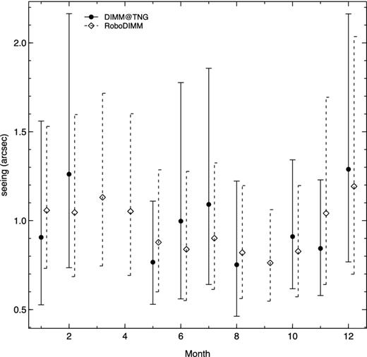
Comparison of the monthly means of the seeing measured by DIMM@TNG (solid lines and solid circles) and RoboDIMM (dashed lines and open diamonds). RoboDIMM data were offset on the x-axis for clarity. The mean values calculated from the logarithmic mean and the error bars correspond to ±1σ of the lognormal monthly distribution.
We also performed a PCA of one year of data of atmospheric variables to compare them with seeing values. We used the data recorded by the TNG weather station, 30 m from the position of DIMM@TNG.
PCA was made using nightly data of air temperature at 10-m above the ground, relative humidity, pressure and the temperature gradient between the 10- and 5-m levels. PC1, which takes account especially of temperature and pressure, explains more than 50 per cent of the variation of the original variables.
The distribution of PC1 shows a bimodal-normal distribution (Fig. 8), with the secondary peak due principally to the months of February, March and April. In Fig. 9 it is possible to note a monthly seasonal trend of PC1, which, with a long-period collection of data, can be used to characterize the seeing distribution according to month or for forecasting.
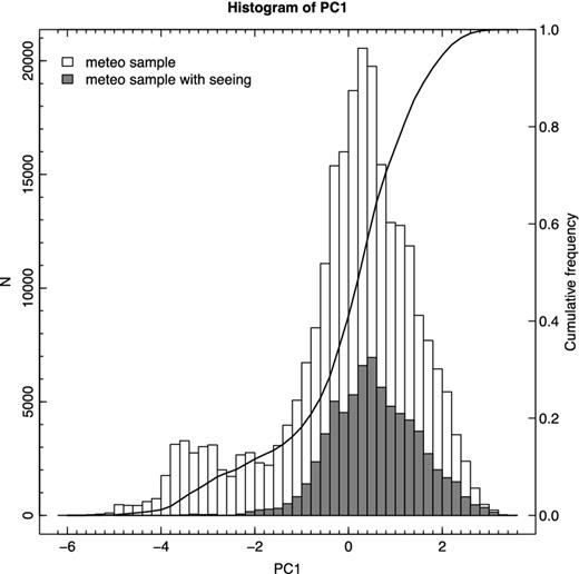
Histograms (left y-axis) and cumulative frequency (right y-axis) of the distribution of PC1 from 2011 March 1 to 2012 March 2. The grey histogram is the subsample of data with seeing measurements.
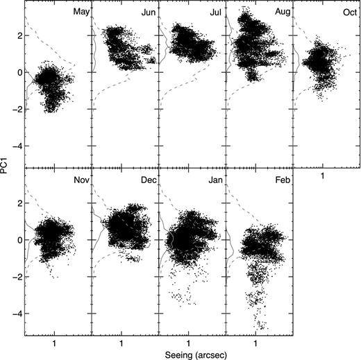
Seeing versus PC1 for each month (2011 September excluded). Dashed lines show the distribution of all PC1 values of the meteorological sample; solid lines show the same distribution for the specific month.
This work was supported by the Italian Istituto Nazionale di Astrofisica (INAF; TECNO2009) and by the Fundación Galileo Galilei of the INAF.
iraf is distributed by the National Optical Astronomy Observatories, which are operated by the Association of Universities for Research in Astronomy, Inc., under cooperative agreement with the National Science Foundation.
