


Abstract
When transiting their host stars, hot Jupiters absorb about 10 per cent of the light in the wings of the stellar Lyman α emission line. The absorption occurs at wavelengths Doppler-shifted from line centre by ±100 km s−1 – larger than the thermal speeds with which partially neutral, ∼104 K hydrogen escapes from hot Jupiter atmospheres. It has been proposed that the absorption arises from ∼106 K hydrogen from the host stellar wind, made momentarily neutral by charge exchange with planetary H i. The ±100 km s−1 velocities would then be attributed to the typical velocity dispersions of protons in the stellar wind – as inferred from spacecraft measurements of the solar wind. To test this proposal, we perform 2D hydrodynamic simulations of colliding hot Jupiter and stellar winds, augmented by a chemistry module to compute the amount of hot neutral hydrogen produced by charge exchange. We observe the contact discontinuity where the two winds meet to be Kelvin–Helmholtz unstable. The Kelvin–Helmholtz instability mixes the two winds; in the mixing layer, charge exchange reactions establish, within tens of seconds, a chemical equilibrium in which the neutral fraction of hot stellar hydrogen equals the neutral fraction of cold planetary hydrogen (about 20 per cent). In our simulations, enough hot neutral hydrogen is generated to reproduce the transit observations, and the amount of absorption converges with both spatial resolution and time. Our calculations support the idea that charge transfer between colliding winds correctly explains the Lyman α transit observations – modulo the effects of magnetic fields, which we do not model but which may suppress mixing. Other neglected effects include, in order of decreasing importance, rotational forces related to orbital motion, gravity and stellar radiation pressure; we discuss quantitatively the errors introduced by our approximations. How hot stellar hydrogen cools when it collides with cold planetary hydrogen is also considered; a more careful treatment of how the mixing layer thermally equilibrates might explain the recent detection of Balmer Hα absorption in transiting hot Jupiters.
1 INTRODUCTION
Gas-laden planets lose mass to space when their upper atmospheres are heated by stellar ultraviolet (UV) radiation. Ubiquitous in the Solar system, thermally driven outflows modify the compositions of their underlying atmospheres over geologic time (e.g. Weissman, McFadden & Johnson 1999). Thanks to the Hubble Space Telescope (HST), escaping winds are now observed from extrasolar hot Jupiters: Jovian-sized planets orbiting at distances ≲0.05 au from their host stars and bathed in intense ionizing fields. Spectroscopy with HST reveals absorption depths of ∼2–10 per cent in various resonance transitions (H i, O i, C ii, Si iii and Mg ii) when the planet transits the star, implying gas outflows that extend for at least several planetary radii (e.g. Vidal-Madjar et al. 2003, 2004, 2008, VM03; Ben-Jaffel 2007, 2008; Fossati et al. 2010; Lecavelier Des Etangs et al. 2010; Linsky et al. 2010). Recent observations of HD 189733b also indicate temporal variations in H i Lyman α absorption, possibly correlated with stellar X-ray activity (Lecavelier des Etangs et al. 2012). These data promise to constrain the compositions of hot Jupiter atmospheres and the degrees to which they are vertically mixed (Liang et al. 2003; Moses et al. 2011).
The HST observations of hot Jupiter winds are accompanied by theoretical studies that model planetary outflows starting from first principles (e.g. Yelle 2004, 2006; Tian et al. 2005; García Muñoz 2007; Murray-Clay, Chiang & Murray 2009, M09). These 1D hydrodynamic models generally agree that hot Jupiters like HD 209458b and HD 189733b are emitting |$\dot{M} \sim 10^{10}$|–1011 g s−1 in mostly hydrogen gas. Three-dimensional (3D) models include Lecavelier des Etangs et al. (2004) and Jaritz et al. (2005), who emphasize the importance of tidal forces.
Do the models agree with the observations? Linsky et al. (2010) find that their observations of C ii absorption in HD 209458b can be made consistent with modelled mass-loss rates, assuming the carbon abundance of the wind is not too different from solar. More comparisons between observation and theory would be welcome – particularly for hydrogen, the dominant component of the wind. But the observations of H i absorption have proven surprisingly difficult to interpret. On the one hand, the original measurements by VM03 indicate substantial (∼10 per cent) absorption at Doppler shifts of ±100 km s−1 from the centre of the H i Lyman α line. On the other hand, theory (e.g. M09) indicates that planetary outflows, heated by photoionization to temperatures T ≲ 104 K, blow only at ∼10 km s−1. How can such slow planetary winds produce significant absorption at ±100 km s−1? Measurements of blueshifted velocities as large as −230 km s−1 in the case of HD 189733b only accentuate this problem (Lecavelier des Etangs et al. 2012).
Holmström et al. (2008, hereafter H08) propose that the observed energetic neutral H atoms arise from charge exchange between planetary H i and protons from the incident stellar wind. In this interpretation, the ±100 km s−1 velocities correspond to the thermal velocities of 106 K hydrogen from the star – hydrogen which is made neutral by electron exchange with planetary H i. The situation is analogous to that of the colliding winds of O star binaries (Stevens, Blondin & Pollock 1992; Lamberts, Fromang & Dubus 2011, and references therein). The H i Lyman α absorption arises from the contact discontinuity where the two winds meet, mix and charge exchange to produce hot neutral hydrogen.
The calculations of H08, and those of the follow-up study by Ekenbäck et al. (2010, hereafter E10), are based on a Monte Carlo algorithm that tracks individual ‘meta-particles’ of neutral hydrogen launched from the planet. The meta-particles collide and charge exchange with stellar wind protons outside a presumed planetary magnetosphere, which is modelled as an ‘obstacle’ in the shape of a bow shock. Good agreement with the Lyα observations is obtained for a range of stellar and planetary wind parameters, and for a range of assumed obstacle sizes.
In this work we further test the hypothesis of charge exchange first explored by H08 and E10. Our methods are complementary: instead of adopting their kinetic approach, we solve the hydrodynamic equations. We do not prescribe any obstacle to deflect the stellar wind, but instead allow the planetary and stellar winds to meet and shape each other self-consistently via their ram and thermal pressures. Some aspects of our solution are not realistic – we ignore the Coriolis force, the centrifugal force, stellar tidal gravity and magnetic fields.1 Our goal is to develop a first-cut hydrodynamic-chemical model of the contact discontinuity between the two winds where material mixes and charge exchanges. Simple and physically motivated scaling relations will be developed between the amount of H i absorption and the properties of the stellar and planetary winds.
The plan of this paper is as follows. In Section 2 we describe our numerical methods, which involve augmenting our grid-based hydrodynamics code to solve the chemical reactions of charge exchange, and specifying special boundary conditions to launch the two winds. In Section 3 we present our results, including a direct comparison with the H i Lyα transit spectra of VM03, and a parameter study to elucidate how the absorption depth varies with stellar and planetary wind properties. A summary is given in Section 4, together with an assessment of the shortcomings of our study and pointers towards future work.
2 NUMERICAL METHODS
In Section 2.1, we describe the hydrodynamics code used to simulate the colliding planetary and stellar winds. In Section 2.2 we detail the charge exchange reactions that were added to the code. In Section 2.3, we outline our post-processing procedure for computing the Lyman α transmission spectrum. As a convenience to readers, in Section 2.4 we re-cap the differences between our treatment of colliding winds and that of E10/H08.
2.1 Hydrodynamics: code and initial conditions
All our simulations are 2D Cartesian in the dimensions x (stellocentric radius) and y (height above the planet's orbital plane). Equivalently the simulations may be regarded as 3D, but with no rotation and with a star and a planet that are infinite cylinders oriented parallel to the z-axis. At fixed computational cost, 2D simulations enjoy better spatial resolution than 3D simulations and thus better resolve the fluid instabilities at the interface of the two winds. The standard box size is (Lx, Ly) = (40Rp, 60Rp), where Rp = 1010 cm is the planet radius. The number of grid points ranges up to (Nx, Ny) = (6400, 9600) (see Table 1).
The star and its wind are modelled after the Sun and the solar wind. The stellar wind is injected through the left edge of the simulation box; the densities, velocities and temperatures in the vertical column of cells at the box's left edge are fixed in time. Stellar wind properties as listed in Table 1 are given for a stellocentric distance r = rlaunch, * = 5 R⊙, near the box's left edge. Here the stellar wind density, temperature, sound speed and flow speed are set to n* = 2.9 × 104 cm−3, T* = 106 K, c* = 129 km s−1 (computed for a mean molecular weight equal to half the proton mass, appropriate for an f+* = 100 per cent ionized hydrogen plasma) and v* = 130 km s−1 (Sheeley et al. 1997; Quémerais et al. 2007; see also Lemaire 2011), respectively. Our stellar wind parameters are such that the implied spherically symmetric (3D) mass-loss rate is 1 × 10¹² g s−1 or 2 × 10⁻¹⁴ M⊙ yr−1.
Parameters of the winds at launch, and of the simulation box.
| Stellar wind | Planetary wind |
|---|---|
| rlaunch, * = 5R⊙ | dlaunch, p = 4Rp |
| n* = 2.9E4 cm−3 | np = 3.9E6/cm3 |
| T* = 1E6 K | Tp = 7000 K |
| v* = 130 km s−1 | vp = 12 km s−1 |
| f+* = 1 | f+p = 0.8 |
| c* = 129 km s−1 | cp = 10 km s−1 |
| M* = 1.01 | Mp = 1.2 |
| Radial (x) direction | Vertical (y) direction |
| Lx/Rp = 40 | Ly/Rp = 60 |
| Nx = 50, 100, 200,400, | Ny = 75, 150, 300, 600, |
| 800, 1600, 3200, 6400 | 1200, 2400, 4800, 9600 |
Our stellar wind parameters are similar to those of the ‘slow’ solar wind in the Sun's equatorial plane. Compare our choices with those of Ekenbäck et al. (2010), who adopt a stellar wind speed of 450 km s−1. Their speed is closer to that of the ‘fast’ solar wind which emerges from coronal holes. At solar minimum, the fast wind tends to be confined to large heliographic latitudes (polar regions), but at solar maximum, the coronal holes migrate to lower latitudes and the fast wind can more readily penetrate to the ecliptic (Kohl et al. 1998; McComas et al. 2003; S. Bale, private communication). Evaporating hot Jupiters like HD 209458b and HD 189733b have orbit normals that are nearly aligned with the spin axes of their host stars (Winn et al. 2005, 2006). Because such planets reside near their stellar equatorial planes, the slow equatorial solar wind seems a better guide than the fast, more polar wind; nevertheless, as noted above, the fast wind is known to extend to low latitudes, and the speeds and densities of both winds vary by factors of order-unity or more with time.
The stellar wind velocity at the left boundary is not plane-parallel but points radially away from the central star (located outside the box). The density, velocity and temperature in each cell at the boundary are computed by assuming that the central star emits a spherical isothermal wind whose velocity grows linearly with stellocentric distance r and whose density decreases as 1/r3. These scalings, which are modelled after empirical solar wind measurements (e.g. Sheeley et al. 1997) and which maintain a constant mass-loss rate with r, are used only to define the left-edge boundary conditions and are not used in the simulation domain. Outflow boundary conditions are applied at the top, bottom and right edges of the box.
As a final comment about our choice of stellar wind parameters, we note that they are valid for the left-edge boundary at r = rlaunch, * = 5 R⊙ – not for the planet's orbital radius of r = 10 R⊙. The left-edge boundary must be far enough away from the planet that the stellar wind properties at the boundary are well-approximated by their ‘free-stream’ values in the absence of any planetary obstacle. We will see in Section 3 that the stellar wind slows considerably between r = 5 R⊙ and r = 10 R⊙ as a consequence of the oncoming planetary wind. This region of deceleration is absent from the models of H08 and E10.
A circle of radius dlaunch, p = 4Rp, centred at position (lx, ly) = (30Rp, 30Rp) (where the origin is located at the bottom left corner of the domain), defines the boundary where the assumed isotropic and radial planetary wind is launched. The properties of our simulated planetary wind, which are similar to those of the standard supersonic models of HD 209458b by García-Muñoz (2007) and Murray-Clay et al. (2009), are listed in Table 1, and are constant in time along the circular boundary. The density and velocity of the planetary wind at this boundary are such that if the wind were spherically symmetric, the mass-loss rate would be 1.6 × 10¹¹ g s−1. This value lies within the range estimated from observations by Linsky et al. (2010) and from energetic considerations (e.g. Lecavelier des Etangs 2007; Ehrenreich & Désert 2011). Note that 1 − f+p = 20 per cent of the planetary wind at launch is neutral (Murray-Clay et al. 2009) and available for charge exchange. This neutral fraction represents a balance between photoionizations by extreme UV radiation and gas advection of neutrals at a planetary altitude of 4–5 Rp (Murray-Clay et al. 2009). The planetary and stellar winds are barely supersonic at launch (Mach numbers Mp = 1.2 and M* = 1.01).
Gravity is neglected, as are all rotational forces. The pressure p is related to the internal energy density e = E − ρV2/2 via p = (γ − 1)e, where γ = 1.01. That is, gas is assumed to behave nearly isothermally. This isothermal assumption should not be taken to mean that the temperature is the same across the simulation domain; the temperature of the stellar wind at injection is T* = 106 K, while that of the planetary wind is Tp = 7000 K.3 Rather, the two winds, as long as they remain unmixed, tend to maintain their respective temperatures as they rarefy and compress. In reality, the stellar wind can keep, in and of itself, a near-isothermal profile on length scales of interest to us because thermal conduction times (estimated, e.g. using the Spitzer conductivity) are short compared to dynamical times. Treating the planetary wind as an isothermal flow is less well justified, as cooling by adiabatic expansion can be a significant portion of the energy budget (García-Muñoz 2007; M09). Nevertheless, the error incurred by assuming the planetary wind is isothermal is small for our standard model because the planetary wind hardly travels beyond its launch radius of 4Rp before it encounters a shock; thus rarefaction factors are small. Furthermore, as noted above, shock compression factors are modest because the speed of the planetary wind is only marginally supersonic. Where the stellar and planetary winds meet and mix, the code ascribes an intermediate temperature 104 K < T < 106 K. This temperature, as computed by heracles, is used only for the hydrodynamic evolution; it is not used for computing either the charge exchange reactions (Section 2.2) or the transmission spectrum (Section 2.3).
Each simulation is performed in two steps. First only the planetary wind is launched from its boundary and allowed to fill the entire domain for 2 × 10⁵ s. Secondly, the stellar wind is injected through the left side of the box, by suitable assignment of ghost cells. This two-step procedure was found to minimize transients. The simulations typically run for 2 × 10⁶ s, which corresponds to ∼60 box-crossing times for the stellar wind in the horizontal direction.
2.2 Charge exchange
Note that in contrast to H08 and E10, our calculations account for the reverse reaction H0h + Hc+ → H+h + Hc0. Accounting for the reverse reaction helps us to avoid overestimating the amount of hot neutral hydrogen. Our calculations of n0h are still overestimated, however, because we neglect thermal equilibration, i.e. cooling of hot hydrogen by collisions with cold hydrogen. In Section 4.1 we estimate the error incurred to be of the order of unity.
Our calculations of the neutral fraction in the mixing layer do not explicitly account for photoionizations by Lyman continuum photons, radiative recombinations or advection of neutral hydrogen from the planetary wind – but these effects are already included by Murray-Clay et al. (2009) whose planetary wind parameters we use (see Section 2.1).
2.3 Lyman α absorption
The transmission spectrum in the Lyman α line is post-processed, i.e. calculated after heracles has finished running. Both hot and cold neutral hydrogen (n0h and n0c) contribute to the Lyman α optical depth. It is assumed that the hot and cold neutral hydrogen do not thermally equilibrate (see Section 4.1 where we question this assumption). Thus, in computing the opacity due to hot hydrogen, we adopt a kinetic temperature of T* = 106 K, and in computing the opacity due to cold hydrogen we take Tp = 7000 K. In each grid cell, the wavelength at line centre is Doppler shifted according to the horizontal component of the bulk velocity (the observer is to the far right of the simulation box). Voigt line profiles are used with a damping constant (Einstein A coefficient) equal to Γ = 6.365 × 10⁸ s−1 (e.g. Verhamme, Schaerer & Maselli 2006).

Snapshots of total density and velocity (left-hand panel), density of hot neutral hydrogen (n0h, middle panel) and temperature (right-hand panel) of the 50×75 simulation, with parameters listed in Table 1. Snapshots are taken at t = 2 × 10⁶ s. The temperature map shown in the right-hand panel is computed by heracles and used only to compute the hydrodynamic evolution; it is not used to compute the charge exchange reactions or the Lyman α spectrum (see Sections 2.2–2.3). The two dashed white lines represent sightlines to the stellar limbs.

2.4 Differences between this work and E10/H08
The main difference between our methods and those of E10/H08 is that we numerically solve the equations of hydrodynamics in a 2D geometry, whereas E10/H08 simulate collisions of hydrogen ‘meta-particles’ in a more kinetic, 3D treatment. Neither we nor they compute magnetic forces explicitly.
E10 include forces arising from the orbit of the planet about the star, including the Coriolis force, the centrifugal force and stellar tidal gravity. We do not. Our focus is on resolving mixing and charge exchange in the interface between the two winds. To that end, we solve for both the forward and reverse reactions of charge exchange (equations 2–3), whereas E10/H08 solve only for the forward reaction. Our equations permit a chemical equilibrium to be established in the mixing layer (see Section 3.2.3). Furthermore, the structure and geometry of the interaction region between the two winds are direct outcomes of our simulations, whereas the shape of the interface layer is imposed as a fixed ‘obstacle’ in the simulations of E10.
Other differences include our treatments of the planetary and stellar winds. We account for both the neutral and ionized components of the planetary wind; E10 assume the planetary outflow is purely neutral. We draw our parameters of the stellar wind from those of the slow equatorial solar wind, which blows at ∼130 km s−1 at a stellocentric distance of r = 5 R⊙ (Sheeley et al. 1997; Quémerais et al. 2007). E10 take the stellar wind to blow at 450 km s−1, while H08 take the stellar wind to blow at 50 km s−1. Neither work accounts for how the stellar wind decelerates due to its interaction with the planetary wind, whereas in our simulations the deceleration zones are well-resolved.
We will review again our simulation methods, and assess the severity of our approximations, in Section 4.1.
3 RESULTS
Results for Lyman α absorption by the mixing layer, including numerical convergence tests and a direct comparison with observations, are given in Section 3.1. A parameter study is described in Section 3.2.
3.1 Absorption versus spatial resolution and time
In Figs 1 and 2, we present results at our lowest (50 × 75) and near-highest (3200 × 4800) spatial resolutions, respectively. The simulations agree on the basic properties of the flow. The planetary wind is launched from the red circle and encounters a bow shock, visible in the left panels as a curved boundary separating orange (unshocked planetary wind) from red (shocked planetary wind). The radius of curvature of the planetary wind shock is roughly ∼6Rp. Outside, the red region of thickness ∼5Rp contains shocked planetary wind.
The stellar wind encounters a weak shock – visible as a near-vertical line separating dark blue from lighter blue in the left-hand panels of Figs 1 and 2 – at a distance of ∼5Rp from the left edge of the box. The shocked stellar wind is diverted around the planet by the pressure at the stagnation point where the two winds collide head on.
We observe that both winds accelerate somewhat before they encounter shocks. For our standard model, the Mach numbers are M* ≲ 1.3 and Mp ≲ 1.5 (for the parameter study simulations of Section 3.2, Mp can grow up to 2–3). Density enhancements are thus modest – less than a factor of 2.
The contact discontinuity between the stellar and planetary winds separates light blue from dark red in the left panels. It is laminar at low resolution but breaks up into turbulent Kelvin–Helmholtz rolls at high resolution (cf. Stone & Proga 2009 whose spatial resolution was probably too low to detect the Kelvin–Helmholtz instability). The middle panels plot the density of hot neutral hydrogen produced by charge exchange in the mixing layer. The ‘head’ of the mixing layer, located near the stagnation point, spans only one or two grid cells in the low-resolution simulation. The high-resolution simulation resolves much better the head of the mixing layer. Zoomed-in snapshots of the head will be presented in Section 3.2.
In Fig. 3, the star-averaged absorption A at an equivalent Doppler velocity of +100 km s−1 (redshifted away from the observer) is plotted against time for a range of spatial resolutions. From t = 0 to 2 × 10⁵ s, the planetary wind fills the simulation domain; the absorption quickly settles down to a value of ∼2 per cent. At these early times, only cold (Tp = 7000 K) neutral hydrogen from the planet is available to absorb in Lyα, and it is clearly insufficient to explain the absorption observed with HST.
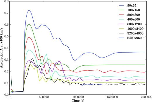
Lyman α absorption A (equation 6), evaluated at a Doppler-shift velocity of +100 km s−1 from line centre, versus time and spatial resolution. The absorption converges in time for all simulations, but only for grid resolutions of 3200 × 4800 or greater does a unique value for the absorption emerge. The 3200 × 4800 simulation is also the lowest resolution run to resolve Kelvin–Helmholtz billows (see Fig. 2).
Starting at t = 2 × 10⁵ s, the stellar wind is injected into the box. The absorption attains a first peak when the planetary and stellar winds reach a rough momentum balance and a mixing layer containing hot (T* = 106 K) neutral hydrogen is established. The height of the first peak decreases with each factor of 2 improvement in grid resolution until a resolution of 3200 × 4800 is reached. Encouragingly, all of the absorption values calculated in the various simulations converge at late times.
The 3200 × 4800 run is the best behaved, with the absorption holding steady at A ≈ 9 per cent for 106 s. Compared to all other simulations at lower resolution, the 3200 × 4800 run is the only one in which Kelvin–Helmholtz rolls appear (more on the Kelvin–Helmholtz instability in Section 3.2.2).
We further tested the convergence of the 3200 × 4800 run by performing an even higher resolution simulation with 6400 × 9600 grid cells. Because of the expense of such a simulation, the initial conditions of the 6400 × 9600 run were taken from the 3200 × 4800 run at t = 106 s, and integrated forward for only 3 × 10⁵ s (approximately nine box crossing times for the stellar wind in the horizontal direction). The absorption values versus time for the 6400 × 9600 run are overlaid in Fig. 3 and are practically indistinguishable from those of the 3200 × 4800 run. Having thus satisfied ourselves that the 3200 × 4800 run yields numerically convergent results, we will utilize this grid resolution (0.0125Rp per grid cell length) for further experiments to understand the dependence of the absorption on input parameters, as described in Section 3.2.
Fig. 4 plots the absorption spectrum for our standard 3200 × 4800 simulation at t = 2 × 10⁶ s. The absorption A is evaluated at wavelengths offset from the central rest-frame wavelength of the Lyman α transition by nine Doppler-shift velocities Δv. Absorption at −50 km s−1 is stronger than at +50 km s−1, a consequence of neutral, charge-exchanged hydrogen from the star accelerating from the stagnation point towards the observer. At larger velocities |Δv| > 100 km s−1, the spectrum is more nearly reflection-symmetric about Δv = 0, because the broadening is purely thermal at T* = 106 K.

Lyman α absorption A versus Doppler-shift velocity Δv from line centre, evaluated for our standard 3200 × 4800 simulation at t = 2 × 10⁶ s. Absorption at −50 km s−1 is stronger than at +50 km s−1 because of the bulk motion of charge-exchanged neutral hydrogen streaming from the star towards the observer. The line wings at larger Doppler shifts are primarily thermally broadened at T* = 106 K. The absorption A ≈ 9 per cent at Δv = ±100 km s−1, in accordance with HST observations (see Fig. 5).
Fig. 5 displays the same information as in Fig. 4 but in the full context of the HST observations. The agreement between the modelled and observed in-transit spectra is encouraging.
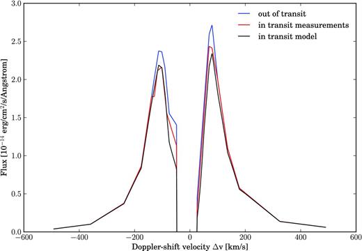
Observed out-of-transit (highest blue curve) and observed in-transit (green curve) Lyman α spectra, reproduced from fig. 2 of Vidal-Madjar et al. (2003). In the line ‘core’ from −42 to +32 km s−1, where interstellar absorption is too strong to extract a planetary transit signal, the flux is set to zero. Our theoretical in-transit spectrum (red curve) is computed by multiplying the observed out-of-transit spectrum by 1 − A, where A is plotted in Fig. 4. The agreement between the theoretical and observed in-transit spectra is good, supporting the idea that charge exchange between the stellar and planetary winds correctly explains the observed absorption at Doppler-shift velocities around ±100 km s−1.
3.2 Scaling relations for absorption in the mixing layer
To understand how absorption in the mixing layer depends on input parameters, we performed three additional simulations varying the launch properties np, n*, vp and Tp. The altered parameters are listed in Table 2. For all three simulations, the box size was maintained at (Lx, Ly) = (40Rp, 60Rp) and the grid resolution was (Nx, Ny) = (3200, 4800).
Launch parameters for the three additional 40Rp × 60Rp simulations at 3200 × 4800 resolution. The stellar parameters v* and T* are kept at their nominal values from Table 1. Note that none of the Mach numbers changes.
| Nominal | np↑ | n*↓ | vp,Tp↑ | |
|---|---|---|---|---|
| n* | 2.9E4 cm−3 | 2.9E4 cm−3 | 9.7E3 cm−3 | 2.9E4 cm−3 |
| np | 3.9E6 cm−3 | 1.2E7 cm−3 | 3.9E7 cm−3 | 3.9E6 cm−3 |
| vp | 12 km s−1 | 12 km s−1 | 12 km s−1 | |$\sqrt{3}\times$|12 km s−1 |
| Tp | 7000 K | 7000 K | 7000 K | 21000 K |
| |$\mathcal {R}$| | |$\mathcal {R}_0$| = 0.11 | |$3\times \mathcal {R}_0$| | |$3 \times \mathcal {R}_0$| | |$3 \times \mathcal {R}_0$| |
Note that our parameter study is not exhaustive. For example, none of the simulations listed in Table 2 varies the Mach number at launch of either the planetary or stellar wind. Actually we have performed simulations varying the Mach number of the stellar wind. These behave as we would expect – in particular, increasing M* increases the amount of absorption because of the increased compression in the stellar shock. Nevertheless, we elect not to include these extra simulations in our parameter study below. Magnetic fields, neglected by our simulations but certainly present in the stellar wind if not also the planetary wind, would stiffen the gas and prevent the kind of compression that we see when we raise M*.
In the following subsections, we explain our numerical results on the properties of the mixing layer with order-of-magnitude scaling relations. The mixing layer's location is analysed in Section 3.2.1; its thickness in Section 3.2.2; the densities of its constituent species in Section 3.2.3; and the column density and absorptivity of hot neutral hydrogen in Section 3.2.4.
3.2.1 Location of the mixing layer
The parameters in Table 2 were chosen to increase |$\mathcal {R}$| by a factor of 3 compared to its value in our fiducial model. By equation (8), when |$\mathcal {R} = 3 \mathcal {R}_0$|, the mixing layer should be displaced three times farther away from the planet compared to its location in our standard model, assuming the star is far enough away that d* is essentially fixed at the star–planet separation. Fig. 6 displays zoomed-in snapshots of the mixing layers for all simulations in Table 2. Looking at the lx-positions of the mixing layers, and recalling that the planet sits at lx = 30Rp, we find that the layer is displaced (30 − 8)/(30 − 21) ≈ 2.4 times farther away in the three new simulations as compared to the standard model. We consider this close enough to our expected factor of 3, given our neglect of the rather thick layers of shocked gas surrounding the mixing layer.

Zoomed-in snapshots of hot neutral hydrogen in the four simulations used to study how the properties of the mixing layer depend on input parameters (see Table 2). Snapshots are taken near t = 2 × 10⁶ for the standard model, and near t = 1 × 10⁶ s for the others. The bottom white dashed line is the line of sight to the lower stellar limb. The upper two red dashed lines bracket the ‘sampling interval’ over which the hot neutral hydrogen density is vertically averaged to produce the density profiles shown in Fig. 7 (the uppermost red dashed line is also the sightline to the upper stellar limb). In cases (b), (c) and (d), the mixing layer is located farther from the planet (centred at lx = 30Rp) than is the case in (a). In cases (b) and (c), the horizontal thickness of the mixing layer is greater than in cases (a) and (d). In case (c), the density of hot neutral hydrogen is lowest. See Section 3.2 for explanations.
Fig. 7 shows density profiles for hot neutral hydrogen in the mixing layer for the three simulations plus our standard model. Densities are averaged over ly and plotted against lx. The fact that the mixing layers in the simulations having |$\mathcal {R} = 3 \mathcal {R}_0$| align in position confirms that |$\mathcal {R}$| is the dimensionless parameter controlling the location of the mixing layer.

Density profiles of charge-exchanged hot neutral hydrogen in the mixing layer, averaged vertically (between the dashed red lines in Fig. 6) and plotted against horizontal position. The planet is located to the right at lx = 30Rp. The mixing layers of the three non-standard simulations are all displaced farther from the planet than in the standard model, a consequence of increasing the ratio |$\mathcal {R}$| of the momentum carried by the planetary wind to that of the stellar wind (Section 3.2.1). The thicknesses of the mixing layers as shown by the red and green curves are larger than those shown by the blue and cyan curves, a consequence of changing the growth rate for the Kelvin–Helmholtz instability (Section 3.2.2). The two dashed lines are predictions of equation (16) based on considerations of chemical equilibrium; the blue, green and cyan curves correctly intersect the upper dashed line, while the red curve correctly intersects the lower dashed line (Section 3.2.3).
3.2.2 Thickness of the mixing layer
3.2.3 Density of hot neutral hydrogen in the mixing layer
3.2.4 Column density and absorptivity of hot neutral hydrogen
As a further check, we show in Fig. 8 the absorption values A to which the four simulations converge. They compare well with the values predicted by (19) using only the launch properties.

Lyman α absorption A versus time, evaluated at a Doppler-shift velocity of +100 km s−1 from line centre, for our standard model plus three additional models with different input parameters as indicated in the legend (see also Table 2). The coloured jagged lines are the results from our numerical simulations. The dashed black lines are the predictions from our physically motivated scaling relation (19); the simulations converge fairly well to the predicted values.
Had we kept the dependence of the mixing layer properties on the stellar wind Mach number M*, equation (16) would be modified such that n0h∝M*2n* – where n* is the pre-shock (launch) density – in accordance with the usual Rankine–Hugoniot jump condition that states that the density increases by the square of the Mach number across a plane-parallel isothermal shock. Equations (17)–(19) would be modified such that A∝N0h∝M*. Indeed, our numerical simulations (not shown) confirm this linear dependence of A on M*. We mention this result only in passing because it is not likely to remain true once we account for the real-life magnetization of the stellar wind. Magnetic fields stiffen gas and reduce the dependence of A on M*.
4 SUMMARY AND DISCUSSION
Using a 2D numerical hydrodynamics code, we simulated the collisional interaction between two winds, one emanating from a hot Jupiter and the other from its host star. The winds were assumed for simplicity to be unmagnetized. Properties of the stellar wind were drawn directly from observations of the equatorial slow solar wind (Sheeley et al. 1997; Quémerais et al. 2007; Lemaire 2011), while those of the planetary wind were taken from hydrodynamic models of outflows powered by photoionization heating (García-Muñoz 2007; Murray-Clay et al. 2009). For our standard parameters, the mass-loss rate of the star is |$\dot{M}_\ast = 2 \times 10^{-14} \,\mathrm{M}_{{\odot }}$| yr−1 = 1012 g s−1 and the mass-loss rate of the planet is |$\dot{M}_{\rm p} = 1.6 \times 10^{11}$| g s−1 = 2.7 × 10⁻³MJ Gyr−1. At the relevant distances, each wind is marginally supersonic – the stellar wind blows at ∼130–170 km s−1 (sonic Mach number M* ≲ 1.3) and the planetary wind blows at ∼12–15 km s−1 (Mach number Mp ≲ 1.5). Thus, shock compression is modest, even without additional stiffening of the gas by magnetic fields.
A strong shear flow exists at the contact discontinuity between the two winds. At sufficiently high spatial resolution, we observed the interfacial flow to be disrupted by the Kelvin–Helmholtz instability. The Kelvin–Helmholtz rolls mix cold, partially neutral planetary gas with hot, completely ionized stellar gas. Charge exchange in the mixing layer produces observable amounts of hot (106 K) neutral hydrogen. Upon impacting the planetary wind, the hot stellar wind acquires, within tens of seconds, a neutral component whose fractional density equals the neutral fraction of the planetary wind (about 1 − f+p = 20 per cent). Seen transiting against the star, hot neutral hydrogen in the mixing layer absorbs ∼10 per cent of the light in the thermally broadened wings of the stellar Lyman α emission line, at Doppler shifts of ∼100 km s−1 from line centre. Just such a transit signal has been observed with the HST (Vidal-Madjar et al. 2003). The ±100 km s−1 velocities reflect the characteristic velocity dispersions of protons in the stellar wind – as inferred from in situ spacecraft observations of the solar wind (e.g. fig. 3 of Marsch 2006).
Our work supports the proposal by Holmström et al. (2008) and Ekenbäck et al. (2010) that charge exchange between the stellar and planetary winds is responsible for the Lyα absorption observed by HST. This same conclusion is reached by Lecavelier des Etangs et al. (2012) in the specific case of HD 189733b. Our ability to reproduce the observations corroborates the first-principles calculations of hot Jupiter mass loss on which we have relied (e.g. Yelle 2004; García-Muñoz 2007; Murray-Clay et al. 2009, M09). Time variations in Lyα absorption are expected both from the variable stellar wind – the solar wind is notoriously gusty – and from the variable planetary wind, whose mass-loss rate tracks the time-variable UV and X-ray stellar luminosity.
4.1 Neglected effects and directions for future research
Although the general idea of photoionization-powered planetary outflows exchanging charge with their host stellar winds seems correct, details remain uncertain. We list below some unresolved issues, and review the effects that our simulations have neglected, in order of decreasing concern.
- Thermal equilibration in the mixing layer. Our calculations overestimate the amount of hot neutral hydrogen produced by charge exchange because they neglect thermal equilibration. A hot neutral hydrogen atom cools by colliding with cold gas, both ionized and neutral, from the planetary wind. The concern is that hot neutral gas cools before it transits off the face of the star. Starting from where the mixing layer is well-developed (say the lower red dashed line in Fig. 6), hot neutral gas is advected off the projected stellar limb in a timeBy comparison, the cooling time is of the order of(20)\begin{equation} t_{\rm adv} \sim 2 R_{\rm p} / v_\ast \sim 2 \times 10^3 \, {\rm s} \,. \end{equation}where n+c is the density of cold ionized hydrogen in the mixing layer, vrel is the relative speed between hot and cold hydrogen, and σ is the H–H+ cross-section for slowing down fast hydrogen, here taken to be the ‘viscosity’ cross-section calculated by Schultz et al. (2008).4 Our estimate of tcool in (21) neglects cooling by neutral–neutral collisions, but we estimate the correction to be small, as n0c is lower than n+c by a factor of 1/(1 − f+p) ∼ 5, and the cross-section for H–H collisions is generally not greater than for H–H+ collisions (A. Glassgold, private communication; see also Swenson, Tupa & Anderson 1985; note that E10 take the relevant H–H cross-section to be 10−17 cm2 but do not provide a reference).(21)\begin{eqnarray} && \!\!\! t_{\rm cool} \sim \displaystyle\frac{1}{n_{\rm c}^+ \sigma v_{\rm rel}} \nonumber\\ && \quad \sim 500 \left( \frac{2 \times 10^6 \, {\rm cm}^{-3}}{n_{\rm c}^+} \right) \left( \frac{ 10^{-16} \, {\rm cm}^2}{\sigma } \right) \left( \frac{100 \,{\rm km\,s^{-1}}}{v_{\rm rel}} \right) \, {\rm s}, \nonumber\\ \end{eqnarray}
That tcool ∼ tadv indicates our simulated column densities of hot neutral hydrogen may be too large, but hopefully not by factors of more than a few. Keeping more careful track of the velocity distributions – and excitation states – of neutral hydrogen in the mixing layer would not only improve upon our calculations of Lyman α absorption, but would also bear upon the recent detection of Balmer Hα absorption in the hot Jupiters HD 209458b and HD 189733b (Jensen et al. 2012).
Magnetic fields. Insofar as our results depend on Kelvin–Helmholtz mixing, our neglect of magnetic fields is worrisome because magnetic tension can suppress the Kelvin–Helmholtz instability (Frank et al. 1996). For numerical simulations of magnetized planetary winds interacting with magnetized stellar winds, see Cohen et al. (2011a,b). These magnetohydrodynamic simulations can track how planetary plasma is shaped by Lorentz forces, but as yet do not resolve how the planetary wind mixes and exchanges charge with the stellar wind.
Dependence of Lyα absorption A on the planetary wind density np. In the same vein as item (ii), we found empirically that A∝n1/2p, and argued that this result arose from the Kelvin–Helmholtz growth time-scale. Ekenbäck et al. (2010) found a much weaker dependence: increasing np by a factor of 100 only increases A in their models by a factor of ∼2 at −100 km s−1 and even less at positive velocities – see their figs 8 and 9. The true dependence of A on np remains unclear.
Rotational effects and gravity. There are a few order-unity geometrical corrections that our study is missing. Our standard stellar wind velocity of v* = 130 km s−1 is comparable to the planet's orbital velocity of vorb = 150 km s−1, so that in reality the stellar wind strikes the planet at an angle of roughly 45°. The Coriolis force will also deflect the planetary wind by an order-unity angle after a dynamical time of r/vorb ∼ 5 × 10⁴ s, by which time the wind will have travelled ∼5Rp from the planet. These geometrical effects are potentially observable [see e.g. Schneiter et al. (2007) and Ehrenreich et al. (2008) for modelling of HD 209458b, and Rappaport et al. (2012) for a real-life example of a transit light curve that reflects the trailing comet-tail-like shape of the occulting cloud]. However, these geometrical effects seem unlikely to change the basic order of magnitude of the absorption A ∼ 10 per cent that we have calculated.
We have also neglected planetary gravity, stellar tidal gravity and the centrifugal force, all of which can change the planetary wind velocity. But this omission seems minor, since we have drawn our input planetary wind velocities from calculations that do account for such forces (M09), at least along the substellar ray. According to fig. 9 of M09, the planetary wind accelerates from vp ≈ 10 km s−1 at a planetocentric distance d = 4Rp, to vp ≈ 30 km s−1 at d = 10Rp. This range of velocities and corresponding distances overlap reasonably well with the range of velocities and distances characterizing our simulations.
Hydrodynamic approximations for the stellar and planetary winds. We have not formally justified our use of the hydrodynamic equations to describe the wind–wind interaction. The problem is that the collisional mean-free path in the stellar wind is much longer than the length scales of the flow: λCoulomb, * = 1/(n*σCoulomb) ∼ 1013(104 cm−3/n*)(10−17 cm2/σCoulomb) cm, where σCoulomb ∼ 10−17(T*/106 K)−2 cm2 is the cross-section for protons scattering off protons. The fact that the solar wind is collisionless and does not necessarily admit a one-fluid treatment is well-known.
Nevertheless, it is perhaps just as well-known that Parker's (1958, 1963) use of the fluid equations to describe the collisionless solar wind is surprisingly accurate, capturing the leading-order features of the actual solar wind. The role of Coulomb collisions in relaxing the velocity distribution functions of protons and electrons is fulfilled instead by plasma instabilities and wave–particle interactions – see e.g. reviews of solar wind physics by Marsch, Axford & McKenzie (2003) and Marsch (2006). The gross properties of collisionless shocks can still be modelled with the hydrodynamic equations insofar as those properties depend only on the macroscopic physics of mass, momentum and energy conservation, and not on microphysics (e.g. Shu 1992).
Note that the planetary wind is fully collisional because of its higher density and lower temperature, and modelling it as a single fluid appears justified: λCoulomb, p ∼ 107(106 cm− 3/np)(Tp/104 K)2 cm, which is smaller than any other length scale in the problem.
Non-Maxwellian behaviour of the stellar proton velocity distribution. Lyman α absorption at the redshifted velocity of +100 km s−1 arises from charge-exchanged neutral hydrogen at the assumed stellar wind temperature of 106 K. We have assumed a Maxwellian distribution function for hydrogen in the stellar wind, and have ignored non-Maxwellian features that have been observed in the actual solar wind, including high-energy tails and temperature anisotropies. Accounting for non-Maxwellian behaviour may introduce order-unity corrections to our results for the absorption. For the more polar fast solar wind, proton temperatures parallel to and perpendicular to the solar wind magnetic field differ by factors of a few at heliocentric distances of 5–10 solar radii (McKenzie, Axford & Banaszkiewicz 1997). For the more equatorial slow solar wind – which our simulations are modelled after – temperature anisotropies are more muted (Marsch et al. 2003, p. 391).
Stellar radiation pressure. Stellar Lyman α photons can radiatively accelerate neutral hydrogen away from the star (e.g. Vidal-Madjar et al. 2003; M09). Both the planetary wind and the charge-exchanged stellar wind in the mixing layer are subject to a radiation pressure force that exceeds the force of stellar gravity by a factor β on the order of unity.
Radiative repulsion of the charge-exchanged stellar wind in the mixing layer may not be observable, because once hot neutral hydrogen is created in the mixing layer, it is advected off the projected limb of the star before radiation pressure can produce a significant velocity: δvrad ∼ GM*/r2 × β × tadv ∼ 6β km s−1, which does not exceed the hot neutral hydrogen's thermal velocity of ∼100 km s−1.
What about radiative acceleration of the planetary wind? The travel time of the planetary wind from the planet to the mixing layer is ∼10Rp/vp ∼ 105 s, long enough for neutral hydrogen to attain radiative blow-out velocities in excess of 100 km s−1. However, the amount of hydrogen that suffers radiative blow-out is limited to the column that presents optical depth unity to Lyman α photons. This column is 1/σline-ctr ∼ 2 × 10¹³(Tp/104 K)1/2 cm−2, and is much smaller than the typical column in the planetary wind, which is (1 − f+p)npRp ∼ 1016 cm−2. Thus the bulk of the planetary wind is shielded from radiative blow-out, and our neglect of radiation pressure appears safe.
Note that Lecavelier des Etangs et al. (2012) find that radiation pressure cannot explain the largest blueshifted velocities observed for HD 189733b; like us, they favour charge exchange.
This project was initiated during the 2011 International Summer Institute for Modelling in Astrophysics (ISIMA) program hosted by the Kavli Institute for Astronomy and Astrophysics (KIAA) at Beijing University. We thank Pascale Garaud and Doug Lin for organizing this stimulating workshop, and Edouard Audit, Stuart Bale, Andrew Cumming, Sebastien Fromang, Pascale Garaud, Astrid Lamberts, Eliot Quataert and Jim Stone for helpful exchanges. We are indebted to Al Glassgold for his guidance in helping us understand H–H and H–H+ collisions, and an anonymous referee for a report that improved the presentation of this paper. ISIMA is funded by the American and Chinese National Science Foundations, the Center for the Origin, Dynamics and Evolution of Planets and the Center for Theoretical Astrophysics at the University of California at Santa Cruz, the Silk Road Project and the Excellence Cluster Universe at TU Munich. Support for EC was provided by NASA through a Hubble Space Telescope Theory grant. This work was given access to the HPC resources of [CCRT/CINES/IDRIS] under the allocations c2011042204 and c2012042204 made by GENCI (Grand Equipement National de Calcul Intensif).
