A ballistic model for a precessing and orbiting jet with a time-dependent ejection velocity

Velázquez, Pablo F.; Raga, Alejandro C.; Cantó, Jorge; Schneiter, E. Matias; Riera, Angels

doi:10.1093/mnras/sts139

Abstract

We have found that the ballistic trajectory of a precessing, orbiting and time-dependent velocity jet has a semi-analytical solution. Bipolar, multipolar and S-like morphologies, which are observed in young protoplanetary and planetary nebula (PPN and PN, respectively), can be reproduced by setting different values for the ratio between dynamical time and precession periods, the ratio between the precession and orbital periods, and the jet velocity variability period. We have also computed numerical simulations and find a good agreement with the semi-analytical solution for a jet 10³ times denser than the surrounding environment.

hydrodynamics, methods: analytical, methods: numerical, ISM: jets and outflows, planetary nebulae: general

1 INTRODUCTION

Collimated outflows or jets ejected by young stars or by the central sources of protoplanetary and planetary nebulae (PPNe and PNe, respectively) can be considered as ballistic if the jet material is much denser than the gas of the circumstellar medium in which the jet propagates. A ballistic model is a good tool for providing restrictions for the parameters employed for describing the morphologies observed in these astrophysical objects.

Masciadri & Raga (2002) carried out an analytical and numerical study of jets launched from a source which follows a circular orbit. They found that this model produces global mirror-like morphologies. The case of a jet launched from a source in an elliptical orbit was explored by González & Raga (2004).

A combination of a precessing and orbiting jet (from a source tracing a circular orbit) was analysed by Raga et al. (2009). They found that the ballistic trajectory of the jet material has an analytical solution, and show that the effects of the orbital motion on the final ballistic trajectory are observed at a distance D_o = v_jτ_o from the jet source. If the orbital period τ_o is lower than the precession period τ_p, a point-symmetric morphology is observed farther away from the central source (due to the precession).

A possible mechanism invoked for explaining the bipolar and multipolar morphologies exhibited by PPNe and young PNe is the presence of a binary system (Bond, Liller & Mannery 1978; Livio, Salzman & Shaviv 1979; Soker & Livio 1994). One of the components of the binary system forms an accretion disc (with material from the companion star) and launches a jet (perpendicular to this disc). The companion star produces a torque on the accretion disc which generates a retrograde precession of the disc/jet system (Terquem et al. 1999). Additionally, a variability of the ejection velocity can be produced if the binary system follows an elliptical orbit, as reported by Witt et al. (2009). Velázquez et al. (2012) considered these elements (binary system and a jet with a time-dependent ejection velocity) and modelled multipolar PPN by means of 3D hydrodynamical simulations.

In this work, we follow the ideas of Masciadri & Raga (2002), González & Raga (2004) and Raga et al. (2009) and find that the case of a precessing, orbiting and time-dependent ejection velocity jet has a semi-analytical solution for its ballistic trajectory (the solution is analytical for the case of a circular orbit). We then compare this ballistic model with results obtained from 3D numerical simulations, which were carried out with the Yguazú-a code. This work is organized as follows: in Section 2 we present the ballistic model, and in Section 3 we give the initial setup of both the ballistic solution and the numerical simulations. The results are shown in Section 4, and finally we present our conclusions in Section 5.

2 BALLISTIC MODEL

As was previously mentioned, the jet material approximately has a ballistic motion if its density is much larger than the density of the surrounding medium. We assume that the jet has a time-dependent ejection velocity v_j(τ). The jet source moves in an elliptical orbit (we also consider the particular case of a circular orbit), and the ejection direction precesses, describing a cone around the orbital (z) axis, with a half-opening angle α. The orbital motion lies on the xy plane, and the precession of the disc+jet system is retrograde with respect to the orbital motion (see Terquem et al. 1999).

The (x, y, z) components of the ejection velocity at time τ, considering both orbital and precession effects, are

\begin{eqnarray} v_{x}(\tau )&=&v_j(\tau ) \sin \alpha \cos (-\omega _{\rm p} \tau +\phi _0) + v_{ox}(\tau ) \end{eqnarray}

(1)

\begin{eqnarray} v_{y}(\tau )&=&v_j(\tau )\sin \alpha \sin (-\omega _{\rm p} \tau +\phi _0) + v_{oy}(\tau ) \end{eqnarray}

(2)

\begin{eqnarray} v_{z}(\tau )&=&v_j(\tau )\cos \alpha , \end{eqnarray}

(3)

where ω_p is the precession angular frequency, ϕ₀ is an initial phase and v_j(τ) is the time-dependent ejection velocity for which we consider a periodic variability of the form

\begin{equation} v_j(\tau )=v_{j0} [1+\Delta v \cos (\omega _o \tau +\delta _0)], \end{equation}

(4)

where ω_o is the orbital frequency (based on Witt et al 2009, we assume the same frequency for the orbital motion and jet velocity variability), v_j0 the mean jet velocity, Δv the half-amplitude (in units of v_j0) and δ₀ the initial phase of the ejection velocity variability. In equations (1) and (2), v_ox and v_oy are the x- and y components of the orbital speed. For a circular orbit, these velocity components are

\begin{equation} v_{ox}= -v_o \sin (\omega _{\rm o} \tau +\gamma _0);\quad v_{oy}= v_{\rm o} \cos (\omega _{\rm o} \tau +\gamma _0), \end{equation}

(5)

where γ₀ is a phase.

We now determine the locus of the ejected material at time t. This material has been ejected at times t > τ, with the velocity components given by equations (1)–(3). At time t, the position of the gas ejected at a time τ is given by

\begin{equation} (x,y,z)=(t-\tau ) (v_x, v_y, v_z). \end{equation}

(6)

Let us call D the distance to the ejected material farthest away from the source, along the symmetry axis of the object. Then, if we set ‘now’ as t = 0, the gas located at a distance D was launched at a time τ = −τ_d, with τ_d = D/(v_max cos α) being the dynamical time of the material at a distance D from the source, and v_max = v_j0(1 + Δv). For τ = −τ_d the precession, orbital and jet velocity variability phases are

\begin{eqnarray} \omega _{\rm p}\tau _{\rm d}+\phi _0=f_0 \end{eqnarray}

(7)

\begin{eqnarray} -\omega _{\rm o}\tau _{\rm d}+\gamma _0=g_0 \end{eqnarray}

(8)

\begin{eqnarray} -\omega _{\rm o}\tau _{\rm d}+\delta _0=d_0, \end{eqnarray}

(9)

respectively. Assuming g₀ = 0, i.e. at τ = −τ_d the binary system is passing through its periastron, and combining equations (7)–(9) with equations (6), we obtain

\begin{eqnarray} x&=& -\tau v_j(\tau ) \sin \alpha \cos [-\omega _{\rm p}(\tau +\tau _{\rm d})+f_0]\nonumber \\ &&+\ \tau v_0 \sin [\omega _{\rm o}(\tau +\tau _{\rm d})] \end{eqnarray}

(10)

\begin{eqnarray} y&=&-\tau v_j(\tau ) \sin \alpha \sin [-\omega _{\rm p}(\tau +\tau _{\rm d})+f_0]\nonumber \\ &&-\tau v_0 \cos [\omega _{\rm o}(\tau +\tau _{\rm d})] \end{eqnarray}

(11)

\begin{eqnarray} z=&-&\tau v_j(\tau )\ {\rm cos}\ \alpha \,, \end{eqnarray}

(12)

where v_j(τ) = v_j0{1 + Δvcos [ω_o(τ + τ_d) + d₀]}.

The following step is to write equations (10)–(12) in a dimensionless form, which can be done by dividing both sides of equations (10)–(12) by D and writing τ as − τ′τ_d (where τ^′ is a dimensionless time). Also we set τ_d = p τ_p and τ_p = q τ_o, where p and q are two dimensionless parameters (following Velázquez et al. 2012).

The q parameter allows us to estimate the mass ratio m₂/m₁ between the two components of the binary system, considering the work of Terquem et al. (1999). Choosing a value for m₁ or m₂, the orbital radius and velocity can be calculated (by using Kepler's third law). Then, the dimensionless form of equations (10)–(12) is

\begin{eqnarray} x^{\prime }&=&\pm \tau ^{\prime } v^{\prime }_{\mathrm j}(\tau ^{\prime }) \tan \alpha \ \cos [\omega ^{\prime }_{\mathrm p}(\tau ^{\prime }-1)+f_0]\nonumber \\ &&+ \tau ^{\prime } v^{\prime }_{\mathrm{o}} \sin [\omega ^{\prime }_{\mathrm{o}}(\tau ^{\prime }-1)] \end{eqnarray}

(13)

\begin{eqnarray} y^{\prime }&=&\pm \tau ^{\prime } v^{\prime }_{\mathrm j}(\tau ^{\prime }) \tan \alpha \ \sin [\omega ^{\prime }_{\mathrm p}(\tau ^{\prime }-1)+f_0]\nonumber \\ &&+\tau ^{\prime } v^{\prime }_{\mathrm o} \cos [\omega ^{\prime }_{\mathrm o} (\tau ^{\prime }-1)] \end{eqnarray}

(14)

\begin{eqnarray} z^{\prime }= \pm \tau ^{\prime } v^{\prime }_{\mathrm j}(\tau ^{\prime })\,, \end{eqnarray}

(15)

with v′_j(τ′) = 1 + Δvcos [ω′_o(τ′ − 1) − d₀]/(1 + Δv) and v′_o = v_o/(v_maxcos α). ω′_p = ω_p τ_d = 2πp and ω′_o = ω_o τ_d = 2πpq are the dimensionless precession and orbital frequencies, respectively. The + (−) sign corresponds to the trajectory of the gas emitted by the jet (counterjet). The solution given by equations (13)–(15) is analytical.

For the case of an elliptical orbit with an eccentricity e and semi-major axis a, v_ox and v_oy have to be evaluated as follows. These velocities can be written as a function of the polar coordinates r and θ (and their derivatives), in the following way:

\begin{eqnarray} v_{\mathrm{ox}}=\dot{r}\, \cos \theta -r \dot{\theta } \sin \theta , \end{eqnarray}

(16)

\begin{eqnarray} v_{\mathrm{oy}}=\dot{r}\, \sin \theta +r \dot{\theta } \cos \theta . \end{eqnarray}

(17)

In order to obtain r and θ as a function of τ, it is necessary to take into account the orbital equation in polar coordinates:

\begin{equation} r=\frac{a(1-e^2)}{1+e\,\cos \theta }. \end{equation}

(18)

Introducing the eccentric anomaly E, this equation can be written as

\begin{equation} r=a (1-e\, \cos E), \end{equation}

(19)

with E being related to the polar angle θ by

\begin{equation} \tan \frac{\theta }{2}=\bigg (\frac{1+e}{1-e}\bigg )^{1/2}\tan \frac{E}{2}. \end{equation}

(20)

The velocities |$\dot{r}$| and |$\dot{\theta }$| can be obtained from equations (18)–(20), resulting in

\begin{eqnarray} \dot{\theta }&=&\bigg (\frac{1+e}{1-e}\bigg )^{1/2}\bigg [\frac{\cos (\theta /2)}{\cos (E/2)}\bigg ]^2 \frac{\omega _{\mathrm o}}{1-e\, \cos E} \end{eqnarray}

(21)

\begin{eqnarray} \dot{r}&=&\frac{a\, e\, \sin \theta \, (1-e^2)}{(1+e\, \cos \theta )^2}\, \dot{\theta }. \end{eqnarray}

(22)

The next step is to obtain E(τ) from Kepler's equation:

\begin{equation} E-e\ {\rm sin}E = \omega _{\mathrm o} \tau +\gamma _0\,. \end{equation}

(23)

As in equation (8), for τ = −τ_d, γ₀ is chosen such that − ω_oτ_d + γ₀ = 0. Writing the right-hand side of equation (23) in a dimensionless form, we have

\begin{equation} E-e\ {\rm sin}E = \omega ^{\prime }_{\mathrm o}(1-\tau ^{\prime })\,. \end{equation}

(24)

In order to calculate v_ox and v_oy we then follow the following procedure:

we solve numerically equation (24) (i.e. by means of a Newton–Raphson method) in order to obtain E(τ), choosing as initial value E(τ) = ω′_o,
we introduce the resulting E(τ) into equation (19) and (20) to obtain r(τ) and θ(τ),
we finally introduce equations (21) and (22) into equations (16) and (17).

We then obtain a dimensionless form for the trajectory, given by equations (10)–(12), for the elliptical orbit case:

\begin{eqnarray} x^{\prime }&=&\pm \tau ^{\prime } v^{\prime }_j(\tau ^{\prime }) \tan \alpha \ \cos [\omega ^{\prime }_{\rm p}(\tau ^{\prime }-1)+f_0]\nonumber \\ &&-\tau ^{\prime } v^{\prime }_{ox}(\tau ^{\prime }) \end{eqnarray}

(25)

\begin{eqnarray} y^{\prime }&=&\pm \tau ^{\prime } v^{\prime }_j(\tau ^{\prime }) \tan \alpha \ \sin [\omega ^{\prime }_{\rm p}(\tau ^{\prime }-1)+f_0]\nonumber \\ &&+\tau ^{\prime } v^{\prime }_{oy}(\tau ^{\prime }) \end{eqnarray}

(26)

\begin{eqnarray} z^{\prime }=\pm \tau ^{\prime } v^{\prime }_{\mathrm j}(\tau ^{\prime })\,. \end{eqnarray}

(27)

3 INITIAL SETUP

3.1 Semi-analytical ballistic model

Employing equations (25)–(27), we have traced several trajectories for the parameters of the models listed in Table 1. As mentioned above, the q parameter allows us to estimate the mass ratio m₂/m₁ between the components of the binary system. Employing equation (1) of Terquem et al. (1999), and choosing the values for e and α, we have calculated τ_p/τ_o versus m₂/m₁ plots, which are displayed in Fig. 1. Using this figure, for each q value listed in Table 1, we can estimate its corresponding m₂/m₁. We have set m₁ = 0.5M_⊙ for all models.

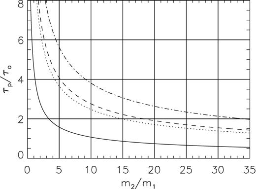
Plot of τp/τo versus m2/m1 for different values of α and e listed in Table 1. The case for α = 5° and e = 0.75 is displayed as a continuous line. The case for α = 15° and e = 0.5 is shown as a dotted line. The curve for the case α = 30° and e = 0.5 is traced as a dashed line, while the case for α = 15° and e = 0 (circular orbit) is plotted as a dot–dashed line.

Figure 1.

Plot of τ_p/τ_o versus m₂/m₁ for different values of α and e listed in Table 1. The case for α = 5° and e = 0.75 is displayed as a continuous line. The case for α = 15° and e = 0.5 is shown as a dotted line. The curve for the case α = 30° and e = 0.5 is traced as a dashed line, while the case for α = 15° and e = 0 (circular orbit) is plotted as a dot–dashed line.

Open in new tab Download slide

Table 1.

Open in new tab

Models.

Models	Δv	p	q	ϵ	m₂/m₁	α(°)	f₀	d₀
M1a	0.5	2	2	0.5	14.8	15.0	0.0	0.0
M1b	0.5	2	2	0.5	14.8	15.0	0.0	− π/2
M1c^a	0.5	2	2	–	14.8	15.0	0.0	− π/2
M1d	0.5	2	2	0.0	33.9	15.0	0.0	− π/2
M2	0.5	2	3	0.5	8.6	30.0	0.0	0.0
M3	0.5	2	4	0.5	5.2	30.0	π/4	0.0
M4	0.5	2	1.5	0.75	5.5	5.0	π/4	0.0
M5	0.25	0.5	6.0	0.5	2.2	15.0	π/4	− π/2

Models	Δv	p	q	ϵ	m₂/m₁	α(°)	f₀	d₀
M1a	0.5	2	2	0.5	14.8	15.0	0.0	0.0
M1b	0.5	2	2	0.5	14.8	15.0	0.0	− π/2
M1c^a	0.5	2	2	–	14.8	15.0	0.0	− π/2
M1d	0.5	2	2	0.0	33.9	15.0	0.0	− π/2
M2	0.5	2	3	0.5	8.6	30.0	0.0	0.0
M3	0.5	2	4	0.5	5.2	30.0	π/4	0.0
M4	0.5	2	1.5	0.75	5.5	5.0	π/4	0.0
M5	0.25	0.5	6.0	0.5	2.2	15.0	π/4	− π/2

^aModels M1c and M1b differ in that the former only considers precession motion.

Table 1.

Open in new tab

Models.

Models	Δv	p	q	ϵ	m₂/m₁	α(°)	f₀	d₀
M1a	0.5	2	2	0.5	14.8	15.0	0.0	0.0
M1b	0.5	2	2	0.5	14.8	15.0	0.0	− π/2
M1c^a	0.5	2	2	–	14.8	15.0	0.0	− π/2
M1d	0.5	2	2	0.0	33.9	15.0	0.0	− π/2
M2	0.5	2	3	0.5	8.6	30.0	0.0	0.0
M3	0.5	2	4	0.5	5.2	30.0	π/4	0.0
M4	0.5	2	1.5	0.75	5.5	5.0	π/4	0.0
M5	0.25	0.5	6.0	0.5	2.2	15.0	π/4	− π/2

Models	Δv	p	q	ϵ	m₂/m₁	α(°)	f₀	d₀
M1a	0.5	2	2	0.5	14.8	15.0	0.0	0.0
M1b	0.5	2	2	0.5	14.8	15.0	0.0	− π/2
M1c^a	0.5	2	2	–	14.8	15.0	0.0	− π/2
M1d	0.5	2	2	0.0	33.9	15.0	0.0	− π/2
M2	0.5	2	3	0.5	8.6	30.0	0.0	0.0
M3	0.5	2	4	0.5	5.2	30.0	π/4	0.0
M4	0.5	2	1.5	0.75	5.5	5.0	π/4	0.0
M5	0.25	0.5	6.0	0.5	2.2	15.0	π/4	− π/2

^aModels M1c and M1b differ in that the former only considers precession motion.

In these models, we have explored the effects of the orbital motion (circular and elliptical: models M1d and M1b, respectively) on the final locus traced by a jet with a time-dependent ejection velocity. Models M1b and M1c allow us to directly compare the cases with precession+orbital motion and with only precession. Also, we have calculated the jet loci obtained by setting the p and q parameters to non-integer values.

3.2 Numerical simulations

In order to compare the results obtained from the semi-analytical method described in the previous section, we also carried out 3D hydrodynamic simulations for some of the models of Table 1.

The 3D numerical simulations were performed with the yguazú-a hydrodynamical code (Raga et al. 2000), which integrates the gas dynamical equations with a second-order accurate scheme (in time and space) using the ‘flux-vector splitting’ method of van Leer (1982) on a binary adaptive grid. A rate equation for neutral hydrogen is integrated together with the gas dynamic equations, and the radiative losses are included with a parametrized cooling function that depends on the density, temperature and hydrogen ionization fraction (Raga & Reipurth 2004). The resulting time-dependent cooling function is plotted in fig. 1 of Velázquez et al. (2011) for a gas parcel that cools at a constant (atom+ion) number density n = 1 cm⁻³.

A computational domain of (1.25, 1.25, 2.5) × 10¹⁷ cm along the x-, y- and z axes (respectively) was employed. An adaptive Cartesian grid with five refinement levels was used, achieving a resolution of ∼4.9 × 10¹⁴ cm at the finest level, corresponding to (256 × 256 × 512) pixels in a uniform grid.

At the centre of the computational domain, we impose a precessing, orbiting and time-dependent ejection velocity jet with a radius of 3.5 × 10¹⁵ cm and a length of 3 × 10¹⁵ cm. Models M1a, M1b, M2, M3, M4 and M5 have been computed employing the parameters listed in Table 1. The initial number density of the jet was set to 10³ cm⁻³, and its mean velocity to 200 km s⁻¹. The jet material propagates into a circumstellar medium with a constant density of 1 cm⁻³ or 10 cm⁻³, in order to compare the results with the predicted trajectories.

4 RESULTS

We obtained the ballistic trajectories for models with the parameters listed in Table 1.

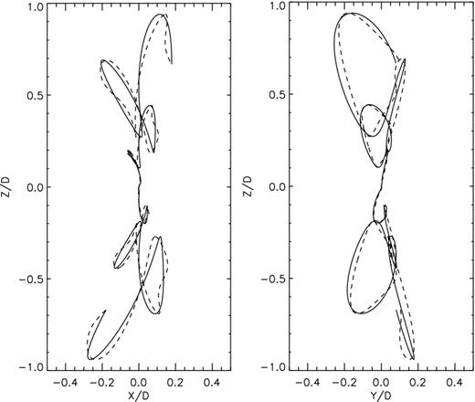
Fig. 2 shows the 3D trajectories traced by models M1a (left) and M1b (right) with solid lines. The projections of the trajectories on the coordinate planes are shown in dashed lines. These models differ from each other in the initial phase of the jet velocity variability. In both models, the projected trajectory on the xz plane traces a point-symmetric quadrupolar shape, and this quadrupolar morphology becomes a bipolar structure for the yz projection of model M1a. In contrast, the yz projection of model M1b shows a wide and well-developed upper lobe and a pair of bottom lobes.

Figure 2.

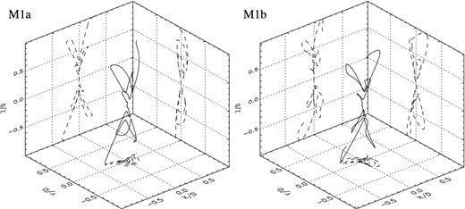
3D ballistic trajectories corresponding to models M1a (left-hand panel) and M1b (right-hand panel). The projections of these trajectory on each three planes are plotted as dashed lines. The axes are given in dimensionless units.

Open in new tab Download slide

The 3D ballistic trajectories obtained from models M2 and M3 are shown in Fig. 3. For model M2, the xz projected trajectory shows a clear point-symmetric quadrupolar morphology, while the yz projection reveals a structure with six lobes. Both projections for model M3 display a quadrupolar morphology, which can be changed by varying the initial phase of the precession motion f₀ (e.g. a six-lobe morphology will be obtained by setting f₀ = 0).

Figure 3.

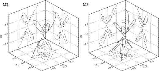
Same as Fig. 2 but for models M2 (left-hand panel) and M3 (right-hand panel).

Open in new tab Download slide

In Fig. 4, we compare the projected trajectories on the xz- and yz-planes for model M1c (solid line) and model M1b (dotted line). Both models share the same parameters with the difference that model M1c only has a precession (and no orbital motion). The trajectories obtained from model M1c show a clear global point-symmetric structure. When we include an elliptical orbital motion, a break on this point-symmetric structure is produced, which is clearly observed on the yz-projected trajectories. In these projections, model M1b exhibits a quadrupolar morphology, while the two upper lobes obtained in model M1b become a single upper lobe in model M1c.

Figure 4.

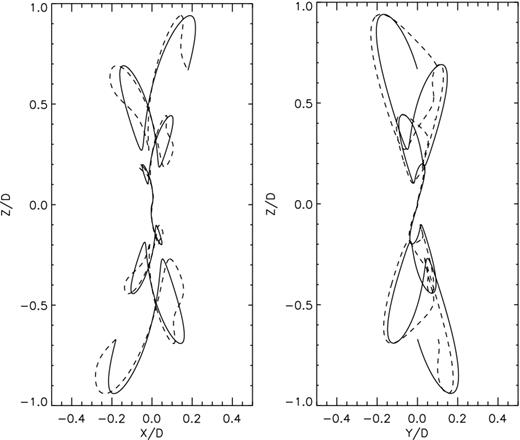
The left-hand panel shows a comparison between trajectories of model M1c (only precession, continuous line) and M1b (precession+orbital motion, dashed line) projected on the xz plane. The right-hand panel shows the yz projection of these trajectories. The axes are given in dimensionless units.

Open in new tab Download slide

The ballistic trajectories obtained for elliptical and circular orbits are compared in Fig. 5 (the projected trajectories for models M1b and M1d are shown with a dashed and a solid line, respectively). Both models show very similar global morphologies.

Figure 5.

The left-hand panel (right-hand panel) shows a comparison between trajectories of models M1d (circular orbit, continuous line) and M1b (elliptical orbit, dashed line) projected on the xz plane (yz plane). Both axes are given in dimensionless units.

Open in new tab Download slide

In order to check the predictions obtained with the semi-analytical calculation, we have also carried out numerical hydrodynamical simulations for all models. After several tests, we found that a good agreement between the numerical simulations and the semi-analytical model is obtained if we consider a ratio between the jet and the environment density greater than 10³, as is shown in Figs 6, 7 and 8. These figures display column-density maps (in grey-scale) obtained from numerical simulations of models M1a and M1b (Fig. 6), M2 and M3 (Fig. 7), and M4 and M5 (Fig. 8). The corresponding ballistic trajectories are also shown in black lines, and they trace very well the locus of the jet material obtained from the numerical simulations. Some departures between the numerical simulations and ballistic trajectories are observed in the case of model M4, mainly in the top-right lobe, where the ballistic trajectory appears ahead of the jet locus obtained from the numerical simulation (see Fig. 7). This departure is produced because the jet gas does not follow a ballistic trajectory when the jet material launched at later times passes through the cocoon generated by the gas emitted at earlier times.

Figure 6.

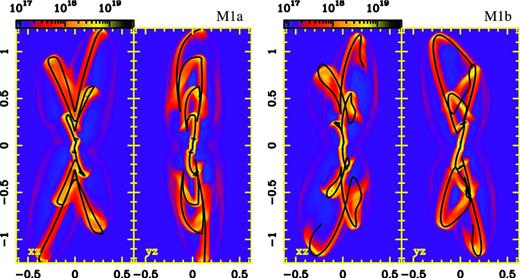
Left-hand panels: xz and yz projections of the column-density maps obtained for model M1a. Right-hand panels: the same but for model M1b. Vertical and horizontal axes are given in units of 10¹⁷ cm, while the logarithmic colour scale is given in cm⁻². The ballistic trajectories obtained for each model are overlayed in white continuous lines.

Open in new tab Download slide

Figure 7.

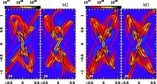
Same as Fig. 6 but left-hand panels showing the column-density maps for model M2, while right-hand panels corresponding to model M3.

Open in new tab Download slide

Figure 8.

Same as Figs 6 and 7 but left-hand panels showing the column-density maps for model M4, while right-hand panels corresponding to model M5.

Open in new tab Download slide

In the previous models, we have considered integer values for the p and q ratios. In models M4 and M5, we explore cases with non-integer p and q values. Fig. 8 shows the column-density maps, in colour scale, obtained from the numerical simulation corresponding to models 4 and 5. The predicted ballistic trajectories of these models are also shown in continuous lines. The xz projection of model M4 resembles the characteristics of the PPN CRL 618 (Riera et al. 2011), while an S-shape is obtained for model M5. This kind of S-shaped morphology is observed in several PPNe and PNe, such as Hen 3-1475 and IC 4634 (Riera, Velázquez & Raga 2004; Guerrero et al. 2008).

5 SUMMARY

We have found that the trajectory of material launched as a precessing and orbiting jet with a time-dependent ejection velocity has a semi-analytical ballistic solution. We find a good fit between this solution and the jet loci obtained through 3D numerical simulations if the initial jet to environment density ratio has a value ≥10³. The ballistic solution is a good tool for exploring the different parameters which are necessary for modelling specific PPNe, young PNe and HH objects with bipolar or multipolar morphologies.

The obtained results confirm that a morphology with well-defined lobes is obtained if a velocity variability of the precessing and orbiting jet (with a half-amplitude of the order of 50 per cent of the mean jet velocity) is considered (see Figs 2–7). The S-like shapes are generated for slowly precessing jets (i.e. with p < 1) as is observed for model M5 in Fig. 8.

This study shows that the effect of the orbital motion is to introduce some departures from the point symmetry due to precession, as is observed in Fig. 4. In addition, the ballistic solution shows that the differences between trajectories obtained considering circular or elliptical orbital motions are not major (Fig. 5).

We conclude by noting that the semi-analytical ballistic solution (for the trajectory of a precessing and orbiting jet, with a time-dependent ejection velocity) is able to reproduce bipolar, multipolar and ‘S-type’ shapes, all of which are observed in some PPNe and HH objects. These morphologies can be obtained considering different values for the ratio between dynamical time and precession period (our p parameter) and for the ratio between the precession and jet velocity variability periods (our q parameter).

†

Member of the Carrera del Investigador Científico, CONICET, Argentina.

The authors thank Enrique Palacios for maintaining the linux servers where the simulations were performed. PFV, ACR and JC acknowledge support from the CONACyT grants 61547, 101356, 101975, 167611, and UNAM DGAPA grant IN105312. The work of ARi was supported by the MICINN grants AYA2008-06189-C03 and AYA 2011-30228-C03.

REFERENCES

Bond

H. E.

Liller

W.

Mannery

E. J.

,

ApJ

,

1978

, vol.

223

pg.

252

Crossref

Search ADS

González

R. F.

Raga

A. C.

,

Rev. Mex. Astron. Astrofis.

,

2004

, vol.

40

pg.

61

Guerrero

M. A.

et al. ,

ApJ

,

2008

, vol.

683

pg.

272

Crossref

Search ADS

Livio

M.

Salzman

J.

Shaviv

G.

,

MNRAS

,

1979

, vol.

188

pg.

1

Crossref

Search ADS

Masciadri

E.

Raga

A. C.

,

ApJ

,

2002

, vol.

568

pg.

733

Crossref

Search ADS

Raga

A. C.

Reipurth

B.

,

Rev. Mex. Astron. Astrofis.

,

2004

, vol.

40

pg.

15

Raga

A. C.

Navarro-González

R.

Villagrán-Muniz

M.

,

Rev. Mex. Astron. Astrofis.

,

2000

, vol.

36

pg.

67

Raga

A. C.

Esquivel

A.

Velázquez

P. F.

Cantó

J.

Haro-Corzo

S.

Riera

A.

Rodríguez-González

A.

,

ApJ

,

2009

, vol.

707

pg.

L6

Crossref

Search ADS

Riera

A.

Velázquez

P. F.

Raga

A. C.

Meixner

M.

Kastner

J. H.

Balick

B.

Soker

N.

,

ASP Conf. Ser. Vol. 313, Asymmetrical Planetary Nebulae III: Winds, Structure and the Thunderbird

,

2004

San Francisco

Astron. Soc. Pac.

pg.

487

Riera

A.

Raga

A. C.

Velázquez

P. F.

Haro-Corzo

S. A. R.

Kajdic

P.

,

A&A

,

2011

, vol.

533

pg.

A118

Crossref

Search ADS

Soker

N.

Livio

M.

,

ApJ

,

1994

, vol.

421

pg.

219

Crossref

Search ADS

Terquem

C.

Eislöffel

J.

Papaloizou

J. C. B.

Nelson

R. P.

,

ApJ

,

1999

, vol.

512

pg.

L131

Crossref

Search ADS

van Leer

B.

Krause

E.

,

Lecture Notes in Physics, Vol. 170, Numerical Methods in Fluid Dynamics

,

1982

Berlin

Springer

pg.

507

Velázquez

P. F.

Steffen

W.

Raga

A. C.

Haro-Corzo

S.

Esquivel

A.

Cantó

J.

Riera

A.

,

ApJ

,

2011

, vol.

734

pg.

57

Crossref

Search ADS

Velázquez

P. F.

Raga

A. C.

Riera

A.

Steffen

W.

Esquivel

A.

Cantó

J.

Haro-Corzo

S.

,

MNRAS

,

2012

, vol.

419

pg.

3529

Crossref

Search ADS

Witt

A. N.

Vijh

U. P.

Hobbs

L. M.

Aufdenberg

J. P.

Thorburn

J. A.

York

D. G.

,

ApJ

,

2009

, vol.

693

pg.

1946

Crossref

Search ADS

Download all slides

Month:	Total Views:
January 2017	1
February 2017	3
March 2017	1
May 2017	1
June 2017	3
August 2017	2
September 2017	3
October 2017	2
November 2017	1
December 2017	9
January 2018	1
February 2018	10
March 2018	8
April 2018	9
May 2018	6
June 2018	5
July 2018	9
August 2018	6
September 2018	5
October 2018	12
November 2018	10
December 2018	6
January 2019	7
February 2019	6
March 2019	11
April 2019	16
May 2019	7
June 2019	6
July 2019	7
August 2019	7
September 2019	3
October 2019	4
November 2019	7
December 2019	5
January 2020	6
February 2020	4
March 2020	8
April 2020	2
May 2020	5
June 2020	6
July 2020	9
August 2020	3
September 2020	7
October 2020	4
November 2020	11
December 2020	3
January 2021	5
February 2021	8
March 2021	10
April 2021	11
May 2021	4
June 2021	7
July 2021	6
August 2021	15
September 2021	5
October 2021	12
November 2021	3
December 2021	1
January 2022	11
February 2022	16
March 2022	13
April 2022	12
May 2022	2
June 2022	4
July 2022	12
August 2022	8
September 2022	9
October 2022	10
November 2022	7
December 2022	6
January 2023	4
February 2023	5
March 2023	1
April 2023	5
May 2023	1
June 2023	1
July 2023	2
August 2023	3
September 2023	1
October 2023	4
November 2023	3
December 2023	7
January 2024	2
February 2024	1
March 2024	3
April 2024	3
May 2024	7
June 2024	8
July 2024	9
August 2024	3
September 2024	3
October 2024	14
November 2024	14
December 2024	8
January 2025	3
February 2025	2
March 2025	8

Article Contents

A ballistic model for a precessing and orbiting jet with a time-dependent ejection velocity

Abstract

1 INTRODUCTION

2 BALLISTIC MODEL

3 INITIAL SETUP

3.1 Semi-analytical ballistic model

3.2 Numerical simulations

4 RESULTS

5 SUMMARY

REFERENCES

Citations

Views

Altmetric

Email alerts

Astrophysics Data System

Citing articles via

Latest

Most Read

Most Cited

Article Contents

A ballistic model for a precessing and orbiting jet with a time-dependent ejection velocity

Abstract

1 INTRODUCTION

2 BALLISTIC MODEL

3 INITIAL SETUP

3.1 Semi-analytical ballistic model

3.2 Numerical simulations

4 RESULTS

5 SUMMARY

REFERENCES

Citations

Views

Altmetric

Email alerts

Astrophysics Data System

Citing articles via

Latest

Most Read

Most Cited

This Feature Is Available To Subscribers Only