


Abstract
Present-day massive galaxies are composed mostly of early-type objects. It is unknown whether this was also the case at higher redshifts. In a hierarchical assembling scenario the morphological content of the massive population is expected to change with time from disc-like objects in the early Universe to spheroid-like galaxies at present. In this paper we have probed this theoretical expectation by compiling a large sample of massive (Mstellar ≥ 1011 h− 270 M⊙) galaxies in the redshift interval 0 < z < 3. Our sample of 1082 objects comprises 207 local galaxies selected from Sloan Digital Sky Survey plus 875 objects observed with the Hubble Space Telescope belonging to the Palomar Observatory Wide-field InfraRed/DEEP2 and GOODS NICMOS Survey surveys. 639 of our objects have spectroscopic redshifts. Our morphological classification is performed as close as possible to the optical rest frame according to the photometric bands available in our observations both quantitatively (using the Sérsic index as a morphological proxy) and qualitatively (by visual inspection). Using both techniques we find an enormous change on the dominant morphological class with cosmic time. The fraction of early-type galaxies among the massive galaxy population has changed from ∼20–30 per cent at z ∼ 3 to ∼70 per cent at z = 0. Early-type galaxies have been the predominant morphological class for massive galaxies since only z ∼ 1.
1 INTRODUCTION
The present-day massive galaxy population is dominated by objects with early-type morphologies (e.g. Baldry et al. 2004; Conselice 2006). However, it is still unknown whether this was also the case at earlier cosmic epochs. Addressing this question is key in our understanding of the physical processes that drive galaxy evolution, as galaxy morphology is directly linked to the evolutionary paths followed by these objects. In fact, a profound morphological transformation of the massive galaxy population is expected within the currently most favoured galaxy formation scenario, the hierarchical model. For massive galaxies this model predicts a rapid formation phase at 2 < z < 6 dominated by a dissipational in situ star formation fed by cold flows (Kereš et al. 2005; Dekel et al. 2009; Oser et al. 2010) and/or gas-rich mergers (Ricciardelli et al. 2010; Wuyts et al. 2010; Bournaud et al. 2011). At the end of this phase, massive galaxies are expected to be more flattened and disc-like than their lower redshift massive counterparts (Naab, Johansson & Ostriker 2009). After this monolithic-like formation phase, massive galaxies are predicted to suffer a period of intense bombardment by minor satellites (Khochfar & Silk 2006; Hopkins et al. 2009; Oser et al. 2010; Feldmann, Carollo & Mayer 2011; Quilis & Trujillo 2012) that may eventually transform the original disc-like population into the predominant present-day spheroid-like population.
Although the above scenario is very suggestive of a deep morphological transformation of the massive galaxy population, there is no compelling observational evidence supporting this idea. However, some recent works suggest that this could be the case (e.g. Oesch et al. 2010; Cameron et al. 2011; van der Wel et al. 2011; Weinzirl et al. 2011; Law et al. 2012). Probing this transformation is difficult from the observational point of view due to the scarce number of massive galaxies at high z. However, the advent of wide area and deep near-infrared surveys (e.g. Dickinson et al. 2003; Scoville et al. 2007; Conselice et al. 2011) have opened up the possibility of exploring a large number of these galaxies up to high redshifts. In this paper we address, to the best of our knowledge for the first time, the issue of the morphological transformation of massive galaxies using a statistical representative sample of nearly ∼1000 galaxies with Mstellar ≥ 1011 h− 270 M⊙ obtained from the Sloan Digital Sky Survey (SDSS) Data Release 7 (DR7) (z ∼ 0; Abazajian et al. 2009), Palomar Observatory Wide-field InfraRed (POWIR)/DEEP2 (0.2 < z < 2; Bundy et al. 2006; Conselice et al. 2007) and GOODS NICMOS Survey (GNS; 1.7 < z < 3; Conselice et al. 2011) surveys. We have already conducted a morphological quantitative analysis of the above galaxies in previous papers (Trujillo et al. 2007; Buitrago et al. 2008) where we have provided clear evidence for a significant size evolution for these objects since z ∼ 3. However, a visual classification of these galaxies and an analysis of their overall profile shape have been missing. In this paper we take advantage of the combined power of the visual and quantitative morphological analysis to explore how the morphologies of the massive galaxy population have changed with redshift.
The structure of the paper is as follows. Section 2 is devoted to the data description and its analysis, Section 3 presents our main results, Section 4 details the evolution with redshift of the various morphological classes and in Section 5 we discuss the implications of our findings. At the end of this work we include an appendix containing the simulations we have performed to test the accuracy of our structural parameter determination in the GNS. Hereafter, we adopt a cosmology with Ωm = 0.3, |$\Omega _\Lambda$| = 0.7 and H0 = 70 km s−1 Mpc−1. We use a Chabrier (2003) initial mass function (IMF) and magnitudes are provided in AB system, unless otherwise stated.
2 DATA
To accomplish our objectives and to be statistically meaningful we need a large number of massive galaxies at all redshifts within our study. Ideally we would also like to study all of our galaxies at a similar rest-frame wavelength range. This is the reason behind our choice of working with several different surveys. The imaging for the local Universe galaxy reference sample was obtained using the SDSS DR7 (Abazajian et al. 2009) although our sample was selected from the NYU Value-Added Galaxy Catalogue (DR6). This catalogue includes single Sérsic (1968) profile fits for 2.65 × 10⁶ galaxies (Blanton et al. 2005), from which 1.1 × 10⁶ galaxies have spectroscopic information. Stellar masses come from Blanton & Roweis (2007), which uses Bruzual & Charlot (2003) models (hereafter BC03) and a Chabrier (2003) IMF. We limited our work to all the massive (M* ≥ 1011 h− 270 M⊙) galaxies with spectroscopic redshifts up to z = 0.03. We have selected this redshift as an upper limit as it contains a local sample with a number of objects (∼200) similar to the number of galaxies we have in our higher redshift bins. On doing this we assure that they are all affected statistically in a similar way. By selecting z = 0.03 we also guarantee that these galaxies are retrieved from a sample that is complete in stellar mass. One object in this local sample was rejected as we discovered it was a stellar spike. Our final local sample contains 207 galaxies. We have used the g-band imaging of SDSS to classify visually our local sample.
In the redshift range 0.2 < z < 2 we utilized the POWIR/DEEP2 survey (Bundy et al. 2006; Conselice et al. 2007, 2008). For this part of the analysis, we restricted ourselves to the Hubble Space Telescope (HST) Advanced Camera for Surveys (ACS) I-band coverage in the Extended Groth Strip (EGS) (see Lotz et al. 2008). It covers 10.1 × 70.5 arcmin, for a total area of 0.2 deg2. The EGS field (63 HST tiles) was imaged with the ACS in the V (F606W, 2660 s) and I band (F814W, 2100 s). Each tile was observed in four exposures that were combined to produce a pixel scale of 0.03 arcsec with a point spread function (PSF) of 0.12 arcsec full width at half-maximum (FWHM). Complementary photometry in the B, R and I bands was taken with the CFH12K camera at the Canada–France–Hawaii Telescope (CFHT) 3.6-m telescope and in the Ks and J bands in a large programme (65 nights) with the WIRC camera at the Palomar 5-m telescope. The depth reached is IAB = 27.52 (5σ) for point sources, and about 2 mag brighter for extended objects. For the purpose of this paper, we have analysed the I-band imaging, although we stress that our sample is K band selected. All the massive galaxies in our sample have KVega < 20, being virtually complete for these objects at z < 2 (Conselice et al. 2007, see section 4.1 and fig. 3). Simulations in Trujillo et al. (2007) agree on the detection of these objects in our ACS imaging.
For the highest redshift bins we used the GOODS NICMOS Survey1 (GNS; Conselice et al. 2011). The GNS is a large HST NICMOS-3 camera program of 60 pointings centred around massive galaxies at z = 1.7-3 at three orbits depth, for a total of 180 orbits in the F160W (H) band. Its total area is 43.7 arcmin2. Each tile (52 × 52 arcsec, 0.203 arcsec pixel−1) was observed in six exposures that were combined to produce images with a pixel scale of 0.1 arcsec, and a PSF of ∼0.3 arcsec FWHM. The limiting magnitude of our observations is HAB = 26.8 (5σ detection in a 0.7 arcsec aperture). The massive galaxies were first identified using a series of selection criteria: Distant Red Galaxies from Papovich et al. (2006), IRAC extremely red objects from Yan et al. (2004) and BzK galaxies from Daddi et al. (2007). There is no photometric method or combination of methods able to perfectly identify a mass-selected sample. Our primary identification, however, finds nearly all massive galaxies that would have been identified in a pure photometric redshift sample, with the exception of apparently rare blue massive galaxies (Conselice et al. 2011). Mortlock et al. (2011) show that the survey imaging is complete for M* ≳ 109.25 M⊙ (corrected to a Chabrier IMF) at z = 3 according to both mass function drops in the number of objects and theoretical predictions from maximally old stellar populations.
2.1 Redshifts and masses, and photometric uncertainties
2.1.1 POWIR/DEEP2
In the POWIR/DEEP2 survey, 795 massive galaxies were used, with 421 of them possessing spectroscopic redshifts (from Davis et al. 2003). There were 35 more massive galaxies in the parent sample, but they were excluded as they are identified as active galactic nucleus (AGN) and hence they may skew our results. When spectroscopic information was not available, photometric redshifts were calculated for the bright galaxies (RAB < 24.1) using the annz code (Collister & Lahav 2004) and bpz (Benítez 2000) for the rest. Accuracy is δz/(1 + z) = 0.025 for z < 1.4 massive galaxies, and δz/(1 + z) = 0.08 for the others (Conselice et al. 2007). Masses were calculated with the method described in Bundy, Ellis & Conselice (2005), Bundy et al. (2006) and Conselice et al. (2007): fitting a grid of model spectral energy distributions (SEDs) constructed from BC03, parametrizing star formation histories by SFR∝exp( − t/τ) (the so-called tau-model; with τ randomly selected from a range between 0.01 and 10 Gyr, and the age of the onset star formation ranging from 0 to 10 Gyr), with a range of metallicities (from 0.0001 to 0.05) and dust contents (parametrized by the effective V-band optical depth τV, where we used values τV = 0.0, 0.5 and 1.2). To analyse the impact of thermal pulsating-asymptotic giant branch (TP-AGB) emission, the same exercise was also performed with Charlot & Bruzual (2007; private communication) models, inferring slightly smaller masses (∼10 per cent). Combining the total uncertainties with those of the photometric redshifts, errors in the masses could be as high as ∼32 per cent for z > 1.4 galaxies (Trujillo et al. 2007). The sample of massive galaxies selected from this survey constitutes the largest sample of HST observed massive galaxies in this redshift range published to date.
2.1.2 GNS
The GNS total sample consist of 80 massive galaxies. We used spectroscopic redshifts (11) when available (Barger, Cowie & Wang 2008; Popesso et al. 2009). Photometric redshifts and masses take advantage of the extensive GOODS fields wavelength coverage (BVRIizJHK), and were obtained using standard multicolour stellar population fitting techniques (Buitrago et al. 2008; Bluck et al. 2009; Conselice et al. 2011), making similar assumptions as in the POWIR/DEEP2 survey about exponentially declining star formation histories, using BC03 and a Chabrier (2003) IMF. Stellar masses errors are typically 0.2–0.3 dex. Spectroscopic redshifts agree well (δz/(1 + z) ∼ 0.03) with photometric determinations (Buitrago et al. 2008). As our observations are probing the optical rest frame (or bluer than this), possible effects by TP-AGB stars are minimized. This sample is the largest massive galaxies compendium (80 objects) at 1.7 < z < 3 imaged with HST we are aware of.
2.1.3 Spectroscopic sample
One of the aims of the present work is selecting a sample with the largest number of spectroscopic redshifts as possible. This is extremely challenging at z > 1.5, even for objects as luminous as massive (M* > 1011 M⊙) galaxies, see e.g. Cimatti et al. (2008). Their spectral features become very difficult to detect, specially when reaching the redshift desert, i.e. when the [O ii] emission line surpasses the 1 μm wavelength limit of optical spectrographs. Consequently, at z < 1.3 two-thirds of our sample posses spectroscopic redshifts, while at higher redshift the number of detections drops to just 10 in POWIR/DEEP2 and 11 in GNS. This fact implies that the redshift bins above z = 1.5 are affected largely by these redshift uncertainties. However, given the quality of our HST photometry and the width of our redshift bins we argue that this has not a crucial impact in our final results.
2.2 Quantitative morphological classification based on the Sérsic index n
We first estimated the apparent magnitudes and sizes of our galaxies using sextractor (Bertin & Arnouts 1996), which were then fed as initial conditions to the galfit code (Peng et al. 2010). galfit convolves Sérsic r1/n 2D models with the PSF of the images and determines the best fit by comparing the convolved model with the observed galaxy surface brightness distribution using a Levenberg–Marquardt algorithm to minimize the χ2 of the fit.
Before we carried out our fitting we masked neighbouring galaxies, following the idea explained in Häußler et al. (2007) and Barden et al. (2012). In the case of very close galaxies with overlapping isophotes, objects were fitted simultaneously. Due to the point-to-point variation of the shape of the camera PSF in our images we chose several (non-saturated) bright stars to gauge the accuracy of our parameter estimations. The final values for the structural parameters of every galaxy are the mean of these independent runs (one per each star used as PSF). The catalogues are published as part of Trujillo et al. (2007; POWIR/DEEP2 sample) and Conselice et al. (2011; GNS sample).
In relation to the SDSS imaging, although the NYU catalogue already provides structural parameters obtained using 1D Sérsic fits to the galaxies, for the sake of consistency with our methodology, we ran again galfit on the SDSS images of these galaxies to obtain structural parameters. It is known that the NYU catalogue has a systematic underestimation of the Sérsic index, effective radius and total flux, as it is reported in the simulations performed in Blanton et al. (2005) and in the appendix of Guo et al. (2009). Our findings agree with this fact, as we find an offset of 26 ± 2 per cent for the circularized effective radius values of our galaxies and another 14 ± 3 per cent for the Sérsic indices. The list of structural parameters of our massive galaxy sample is given in online supporting information.
We performed simulations to assess the reliability of our quantitative results at high redshift. Our purpose was two-folded: correcting our structural parameters for a more accurate representation of their values and exploring in an unbiased way whether we are missing any region in the parameter space of the massive galaxy properties. In the case of the POWIR/DEEP2 sample the simulations are fully explained in Trujillo et al. (2007). They created 1000 artificial galaxies with random structural properties within the observed ranges of the sample. In that study no significant trend in either the sizes or the concentration of the galaxies was found (see their fig. 3), except for an underestimation of ∼20 per cent in the Sérsic index of the very faint IAB > 24 spheroid-like galaxies. We carried out a similar analysis in Appendix A for the galaxies in the GNS sample. For this paper, we went a step further in the complexity of our simulations, not only in the number of objects (×16) but specially in finely sampling the small sizes regime (0.15–0.3 arcsec) which is key to understanding the compact massive galaxy population.
Here we offer a brief description of our simulations. We created 16 000 mock galaxies employing the idl routines developed for Häußler et al. (2007), randomizing both the galaxy positions in our imaging and the galaxy structural parameters. Once the output of our simulations in the parameters space (Houtput, re, output, noutput) was recovered, we estimated the difference with the intrinsic (input) values. The most important outcome is that, on average, the Sérsic indices of our observed GNS massive galaxies grow by ∼10 per cent when corrections based on the simulations are applied. However, the individual values per galaxy depend on its exact position in the 3D space defined by the apparent magnitude, Sérsic index and effective radius.
In general, we found that for objects with disc-like surface brightness profiles (i.e. ninput < 2.5), both sizes and Sérsic indices are recovered with basically no bias down to our limiting explored H-band magnitude. However, by increasing the input Sérsic index we found biases in the determination of the sizes and n. For example, a galaxy with ninput ∼ 4 and H = 22.5 mag (our median magnitude within the GNS catalogue), the output effective radii are ∼10 per cent smaller and output Sérsic indices are ∼15–20 per cent smaller than the input values. The results of these simulations, however, show that the decrease in the Sérsic index we observe from z ∼ 2.5 to z = 0 for the spheroid-like population (which is around a factor of ∼2) cannot be fully explained as a result of the bias on recovering the Sérsic index.
2.3 Qualitative visual morphological classification
In addition to the quantitative morphological analysis explained above, visual morphological classifications were derived for all the galaxies in our sample. To assure a high reliability in our results, two authors of this paper (Fernando Buitrago and Ignacio Trujillo, with checks by Christopher J. Conselice) classified visually all the galaxies in an independent way. We divided our sample according to the Hubble classification scheme into spheroid-like objects (E+S0 or early type), disc-like objects (S or late type) and peculiar galaxies (either irregular galaxies or ongoing mergers). In Fig. 1 we show some examples of our classification scheme at different redshifts. Very conspicuous bulge systems were identified as early-type objects. Both E and S0 galaxies are hence included together in the same morphological class. We avoid segregating between E and S0 since, at high z, it is a difficult task to distinguish between these two types of galaxies, and we prefer to remove this potential source of error. Spiral or late-type morphologies are detected by a central brightness condensation located at the centre of a thin disc containing more or less visible spiral arms of enhanced luminosity. Finally, we joined irregular (unsymmetrical) galaxies and mergers in the same class, again to avoid any misclassification at high z where the differences between these types are more difficult to interpret.
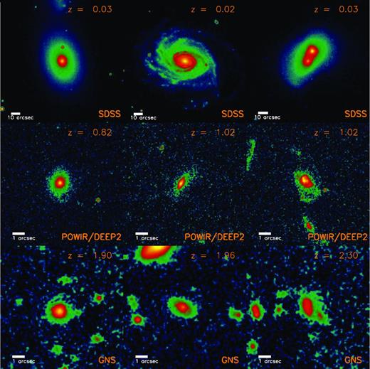
Some examples illustrating our morphological criteria (columns) for different galaxies in our sample. Each row shows galaxies from the different surveys. Please note the different scales of each image due to the different redshift coverage of each survey (lower left-hand corner); according to the cosmology used in this work, 10 arcsec in SDSS are ∼6 kpc at z ∼ 0.03, while 1 arcsec in the HST imaging at z ≥ 1 is ∼8 kpc. Despite the decrease in angular resolution and the cosmological surface brightness dimming with redshift, the exquisite HST depth and resolution (∼10 times better than ground-based SDSS imaging) allow us to explore the morphological nature of the high-z galaxies. Note that irregulars and mergers are in the same morphological class (peculiars).
It is not straightforward to asses the robustness of our visual classifications as this is a pattern recognition problem and as such cannot be addressed by standard algorithm procedures. Nevertheless, at z ∼ 0, we can compare our results with other alternatives coming from independent studies. First, we compare our results with the SDSS Bayesian automated morphological classification by Huertas-Company et al. (2011). There are 190 out of our 207 galaxies in common where we can make a direct comparison. They applied support vector machine techniques (Huertas-Company et al. 2008) to associate a probability to each galaxy being E, S0, Sab or Scd. For those galaxies where they have assigned a probability larger than 90 per cent of pertaining to a given class, their neural network agrees with our visual classification for 89 per cent of the early types and 68 per cent of the late types. Moreover, all our SDSS local galaxies have been visually classified within the Galaxy Zoo project (Lintott et al. 2011). We find that 112 out of the 121 galaxies that we classified as early type are classified as ellipticals by Galaxy Zoo (i.e. ∼93 per cent). For spiral galaxies we get 48 out of 62 (i.e. ∼77 per cent). The discrepancies in our late-type galaxies identifications arise from the difficulty to interpret S0 galaxies without the astronomer's ‘trained-eye’ intervention and, as stated previously, they are included as early-type objects throughout our study. Consequently, our local classification seems to be robust.
2.4 Potential observational biases
We acknowledge, however, that at higher redshifts visual morphological classification is more controversial for several reasons. First, the cosmological surface brightness dimming may affect the recognition of fainter galactic features and secondly, the angular resolution is poorer at higher redshift. Nonetheless, the first effect is compensated by the increase of the intrinsic surface brightness (e.g. Marchesini et al. 2007; Prescott, Baldry & James 2009; Cirasuolo et al. 2010) of the galaxies due to having a higher star formation rate (SFR) in the past, and the fact that their stellar populations are younger. In relation to the angular resolution, at z = 0.03, 1 arcsec is equivalent to ∼0.6 kpc, whereas at 1 < z < 3 it is ∼8.0 kpc. Fortunately, the higher resolution imaging used for exploring the morphologies of our high-z galaxies (FHWM ∼ 0.1–0.3 arcsec) compared to the local ones (FWHM ∼ 1.0–1.5 arcsec) alleviates this problem, although in general, a smoother surface brightness distribution due to the worse resolution is expected. All these effects combined imply that at higher redshifts there would be a larger number of featureless objects that visually would be confused with early-type galaxies. We will show in the next section that this is the opposite of what we find, ultimately giving stronger support to the results of this paper.
Another source of uncertainty comes from the objects catalogued as peculiar class. This classification could be seen as a miscellaneous box where we included galaxies which do not fulfil neither early-type nor late-type descriptions. Furthermore, their photometry may be compromised by means of their multiple components. For the sake of clarity, we include here the number of irregular massive galaxies in our redshift bins (see Table 1) which is 2/0/11/27/14/8, while for mergers are 5/8/31/31/16/13. The aim of this paper is not to constrain the nature of this peculiar class, and due to the multiple nature of some of their members their results are only tentative.
Finally, we must bear in mind that dust obscuration may alter galaxy observables depending on the geometry. Its main effect is usually an artificial size increment and Sérsic index lowering due to the fact that central concentrations of dust flatten the flux profile from the observed galaxy (Trujillo et al. 2006). In reality, the real contribution depends on the amount of dust and its distribution within the galaxies at study (see Möllenhoff, Popescu & Tuffs 2006, where the authors also present corrections for discs scalelenghts and central surface brightnesses). However, both Trujillo et al. (2007) (see their fig. 4 and section 4.2) and Buitrago et al. (2008) (see their section 4) reported only small changes in the structural parameters when comparing ACS and NICMOS observations. We shall come back to this issue in more detail in our next section.
2.5 Morphological K-corrections
The K-correction effect is another potential source of error both within the quantitative and visual morphological classification. We have selected our filters at each survey to minimize this effect, and to observe the galaxies as close as possible to the optical rest frame. Nonetheless, our classification at 1.3 ≲ z ≲ 2 could be compromised by using F814W as this filter is tracing the ultraviolet (UV) rest frame of our targets.
We explored how relevant this effect is by analysing the properties of 24 galaxies with z < 2 in our POWIR/DEEP2 sample which also have H-band NICMOS imaging. In Trujillo et al. (2007), we discussed the size difference between the optical and near-infrared for these galaxies (their fig. 4). We did not find a systematic bias, but a scatter of 32 per cent. With regards to the Sérsic index, we found an offset of 30 ± 9 per cent towards larger indices in the H band. The difference in the visual morphology between the I and the H bands shows that 19 galaxies (79 ± 8 per cent) have the same morphology in the two filters, while only five (21 ± 8 per cent) are catalogued differently. Our errors for visual classifications are represented by the standard deviations for a binomial distribution. We found in ACS 13 (54 ± 10 per cent) early-type galaxies (10 in NICMOS, 42 ± 10 per cent), six (25 ± 9 per cent) late-type galaxies (10 in NICMOS, 42 ± 10 per cent) and five (21 ± 8 per cent) peculiar galaxies (four in NICMOS, 17 ± 8 per cent).
In addition to this analysis of galaxies in the EGS, we compared the difference between the I- and H-band morphologies for those galaxies in the GNS with 1.7 < z < 2 (which is the redshift interval where our POWIR/DEEP2 and GNS sample overlap). We used the I-band ACS imaging of the GOODS fields (Giavalisco et al. 2004). Postage stamp images for 20 common galaxies were retrieved from the rainbow data base (Barro et al. 2011). Our galfit analysis showed that the effective radius and the Sérsic index are recovered without any significant offset, but with a large scatter as in the aforementioned Trujillo et al. (2007). Regarding their visual morphologies, we found that six galaxies (30 ± 10 per cent) were not possible to classify reliably due to the few pixels that compose their image, most probably due to dust obscuration (Buitrago et al. 2008; Bauer et al. 2011). For the remaining 14 galaxies, 11 (55 ± 11 per cent) have the same visual morphology, while for three galaxies (15 ± 8 per cent) there is a difference. For the detections in the ACS camera, foour (28 ± 12 per cent) are early types (six for their NICMOS counterparts, 43 ± 11), six (43 ± 11 per cent) are late types (five in NICMOS, 36 ± 13 per cent) and four (28 ± 12 per cent) are peculiars (three in NICMOS, 21 ± 11 per cent).
There are a number of studies which have explored the K-correction issue for massive galaxies. Toft et al. (2007) analysed a sample of 41 galaxies with masses greater than 1010 M⊙ at 1.9 < z < 3.5 having NICMOS and ACS imaging as well. They reported that half of their Distant Red Galaxies where marginally detected or even disappeared in rest-frame UV bands. In contrast, Cassata et al. (2011) reported a weak K-correction within their 563 similar-mass passive galaxies comparing ACS and Wide Field Camera 3 (WFC3) observations. Our sample is not as high redshift as Toft et al. (2007), it is more massive on average and in addition we deal a variety of massive galaxies instead of red and passive galaxies as in Cassata et al. (2011). Summarizing, K-correction undoubtedly plays a role, which is hard to delimit in our sample. Nevertheless, our tests help us understanding that visual morphologies appear to be robust against these changes.
2.6 Axis ratios
Finally, we can conduct a further test to quantify the robustness of our visual classification, namely to explore the axis ratio distribution of our objects. The axis ratio distribution of local disc galaxies has a mean value of ∼0.5 (Ryden 2004). On the other hand, the axis ratio distribution of the nearby E/S0 population is known to peak at around 0.7–0.8 (Ryden et al. 2001). Fig. 2 displays the distributions of axis ratios in our sample according to our visual morphological determinations. We also overplot the median values from our samples (dashed line) and the axis ratio distribution using only our local sample (dotted line). In Table 1 we also show the mean axis ratio for our different galaxy populations. We find that the objects that are visually classified as early-type galaxies have a typical axis ratio of ∼0.7 (independent of their redshift). Also, for galaxies visually classified as discs, the axis ratio is independent of the redshift with an average b/a ∼ 0.55. Both values are in good agreement with the expectation from the local Universe. This test reinforces the idea that our visual classifications are accurate.
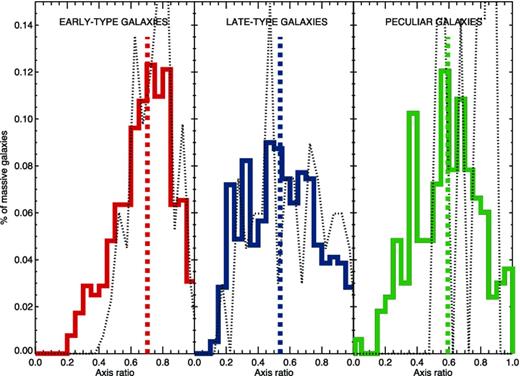
Axis ratio distributions for our whole sample of massive galaxies according to their visual morphology. Vertical dashed lines are the median values of each histogram (0.70, 0.54 and 0.59, respectively). In order to have a local reference, we also overplotted our SDSS sample axis ratio distribution using the thin dotted line. The axis ratio distribution for the discs is rather symmetrical, but this is not the case for early-type objects, which peak at higher axis ratio values. Van der Wel et al. (2011) argued that massive galaxies with axis ratios ≲0.5 are most probably related with late-type objects, as this histograms confirm. Interacting/peculiar galaxies should be taken out of these considerations. The histograms are also in agreement with the estimations of axis ratio distributions for local early-type and late-type objects (Ryden, Forbes & Terlevich 2001; Ryden 2004). This fact highlights the reliability of our visual morphological classification.
Observed mean structural parameters (± the standard deviations) for visually classified massive (M* > 1011 h− 270 M⊙) galaxies at 0 < z < 3.
| Redshift range | Number of galaxies | Survey | Effective radius (kpc) | Sérsic index | Axis ratio (b/a) | Mean stellar mass (× 1011 h− 270 M⊙) |
|---|---|---|---|---|---|---|
| Early-type galaxies | ||||||
| 0–0.03 | 133 | SDSS | 7.15 ± 1.56 | 4.83 ± 1.19 | 0.74 ± 0.13 | 1.26 ± 0.22 |
| 0.2–0.6 | 44 | POWIR | 4.77 ± 2.05 | 5.57 ± 1.46 | 0.71 ± 0.15 | 1.51 ± 0.45 |
| 0.6–1.0 | 184 | POWIR | 3.52 ± 1.79 | 5.13 ± 1.41 | 0.67 ± 0.19 | 1.78 ± 0.69 |
| 1.0–1.5 | 104 | POWIR | 2.06 ± 1.04 | 4.39 ± 1.32 | 0.63 ± 0.19 | 1.70 ± 0.51 |
| 1.5–2.0 | 30 | POWIR | 1.31 ± 0.73 | 3.97 ± 1.38 | 0.65 ± 0.17 | 1.56 ± 0.37 |
| 1.7–3.0 | 25 | GNS | 1.30 ± 0.55 | 2.73 ± 0.96 | 0.68 ± 0.11 | 1.58 ± 0.42 |
| Late-type galaxies | ||||||
| 0–0.03 | 67 | SDSS | 8.44 ± 3.28 | 2.71 ± 1.19 | 0.60 ± 0.22 | 1.21 ± 0.14 |
| 0.2–0.6 | 26 | POWIR | 5.39 ± 1.77 | 2.62 ± 1.28 | 0.50 ± 0.25 | 1.40 ± 0.30 |
| 0.6–1.0 | 124 | POWIR | 4.91 ± 2.04 | 1.86 ± 0.98 | 0.54 ± 0.21 | 1.53 ± 0.49 |
| 1.0–1.5 | 95 | POWIR | 4.81 ± 1.90 | 1.53 ± 0.87 | 0.57 ± 0.23 | 1.58 ± 0.41 |
| 1.5–2.0 | 42 | POWIR | 3.88 ± 1.51 | 1.20 ± 0.73 | 0.50 ± 0.20 | 1.61 ± 0.49 |
| 1.7–3.0 | 34 | GNS | 2.55 ± 1.18 | 1.38 ± 0.62 | 0.54 ± 0.18 | 1.55 ± 0.50 |
| Peculiar galaxies | ||||||
| 0–0.03 | 7 | SDSS | 8.39 ± 2.22 | 3.17 ± 0.61 | 0.72 ± 0.13 | 1.16 ± 0.13 |
| 0.2–0.6 | 8 | POWIR | 4.93 ± 2.26 | 4.95 ± 2.04 | 0.56 ± 0.23 | 1.16 ± 0.08 |
| 0.6–1.0 | 42 | POWIR | 4.16 ± 2.39 | 3.05 ± 2.40 | 0.56 ± 0.20 | 1.65 ± 0.49 |
| 1.0–1.5 | 58 | POWIR | 3.83 ± 1.64 | 1.96 ± 1.62 | 0.61 ± 0.18 | 1.65 ± 0.51 |
| 1.5–2.0 | 30 | POWIR | 2.53 ± 1.68 | 1.70 ± 1.36 | 0.53 ± 0.26 | 1.81 ± 0.68 |
| 1.7–3.0 | 21 | GNS | 2.45 ± 1.04 | 1.69 ± 1.31 | 0.61 ± 0.18 | 1.44 ± 0.34 |
3 RESULTS
The evolution of galaxy morphology with redshift can be addressed in two different ways: quantitative (exploring how their structural parameters have changed with time) and qualitative (probing how the visual appearance has evolved with redshift). In the local Universe, the structural properties of massive galaxies (mainly its light concentration) can be linked with their appearance. In particular, as a first approximation one can identify disc or late-type galaxies with those galaxies having lower values of the Sérsic index (n ∼ 1; Freeman 1970) and early-type galaxies with those having a profile resembling a de Vaucouleurs (1948) shape (n ∼ 4). This crude segregation based on the Sérsic index was shown to work reasonably well by Ravindranath et al. (2004). Whether this equivalence also holds at higher redshift is not clear, and in this paper we explore this issue.
Table 1 lists the mean values of the structural parameters from the galaxies in our sample, splitting them among a number of redshift ranges and their visual morphologies. Concerning effective radius measurements, we retrieve again the reported size decrease for massive galaxies with redshift. As explained in Section 2.6, axis ratio values per morphological class are independent of redshift, which agree with our morphological classifications. Finally, there is a tendency for the Sérsic indices (observed using both mean and median values, see Fig. 3) to become progressively smaller at increasingly higher redshifts. Moreover, there is a separation in the average Sérsic index for late- and early-type massive galaxies at all redshifts. Due to the number of photometric redshifts we used, it is interesting to know whether all these statistical tendencies are preserved if only taken into account the results for galaxies with spectroscopic redshifts. This is in fact the case and it is presented in Table 2.
Observed mean structural parameters (± the standard deviations) for visually classified massive (M* > 1011 h− 270 M⊙) galaxies with spectroscopic redshifts at 0.2 < z < 1.5.
| Redshift range | Number of galaxies | Survey | Effective radius (kpc) | Sérsic index | Axis ratio (b/a) | Mean stellar mass (× 1011 h− 270 M⊙) |
|---|---|---|---|---|---|---|
| Early-type galaxies | ||||||
| 0.2–0.6 | 36 | POWIR | 4.86 ± 2.07 | 5.73 ± 1.51 | 0.73 ± 0.14 | 1.51 ± 0.46 |
| 0.6–1.0 | 124 | POWIR | 3.54 ± 1.88 | 5.19 ± 1.37 | 0.68 ± 0.19 | 1.83 ± 0.74 |
| 1.0–1.5 | 41 | POWIR | 2.16 ± 1.24 | 4.61 ± 1.34 | 0.66 ± 0.17 | 1.91 ± 0.61 |
| Late-type galaxies | ||||||
| 0.2–0.6 | 12 | POWIR | 5.48 ± 1.48 | 2.90 ± 1.22 | 0.58 ± 0.27 | 1.49 ± 0.30 |
| 0.6–1.0 | 68 | POWIR | 5.09 ± 2.11 | 1.97 ± 1.12 | 0.60 ± 0.21 | 1.42 ± 0.37 |
| 1.0–1.5 | 40 | POWIR | 4.45 ± 1.92 | 1.46 ± 0.81 | 0.62 ± 0.23 | 1.56 ± 0.38 |
| Peculiar galaxies | ||||||
| 0.2–0.6 | 5 | POWIR | 5.25 ± 2.37 | 5.12 ± 2.40 | 0.43 ± 0.15 | 1.16 ± 0.09 |
| 0.6–1.0 | 22 | POWIR | 3.79 ± 2.11 | 2.99 ± 2.20 | 0.60 ± 0.21 | 1.64 ± 0.49 |
| 1.0–1.5 | 24 | POWIR | 4.37 ± 2.23 | 1.38 ± 1.13 | 0.65 ± 0.20 | 1.88 ± 0.70 |
We show in Fig. 4 the Sérsic index distribution for our different visually classified morphological types as a function of redshift. It is noteworthy that we had applied to this figure and to the next ones (unless otherwise stated) the corrections for the GNS (see Appendix A), and also for the POWIR/DEEP2 data using Trujillo et al. (2007) simulations. They only affect the two highest redshift bins. For the sake of clarity, we also display in Fig. 5 these histograms without any corrections. We do not appreciate that our corrections based on simulations affect the main results of our paper.
Coming back to Fig. 4, massive galaxies identified visually as late types show low Sérsic index values at all redshifts. This reinforces the idea that the stellar mass density distributions of rotationally supported systems are close to an exponential profile. However, the distribution of the Sérsic index for these late-type galaxies shows a tail towards larger values. This is normally interpreted as the result of the bulge component. In fact, the excess of light caused by the bulge at the centre of the disc will increase the value of this concentration parameter when the galaxies are fitted just using a single Sérsic model. Interestingly, we observe that at higher redshift the prominence of this tail of higher Sérsic indices decreases for the late-type galaxies.
One could be tempted to interpret this result as a consequence of the disappearance of prominent bulges at higher redshifts. However, a full exploration of this bulge development issue is beyond the scope of this paper. In the same Fig. 4, we show the distribution of the Sérsic index for massive galaxies visually classified as early types. We see that at low redshift, the distribution of Sérsic indices for these galaxies predominantly show large values of concentration as expected. Up to z ∼ 1.5 there is a peak around n ∼ 4–6 (see also Table 1). A general trend is also observed: there is a progressive shift towards lower and lower Sérsic index values as redshift increases.
We conducted a series of Kolmogorov–Smirnov (KS) tests in order to check the significance of the changes in the Sérsic index with redshift. In Fig. 6 we show the evolution of the KS significance levels for the different morphological types in our sample of massive galaxies. The KS test is a non-parametric method of comparing probability distributions. We used as a base comparison the lowest redshift bin Sérsic index distribution (left-hand panel), and the highest redshift one (right-hand panel). Despite the uncertainties, mainly due to the number statistics, it seems that the distributions of Sérsic indices gradually change from low to high redshift, and vice versa. When we conduct the analysis using the high-z bin as the reference instead of the local one, the evolution of the Sérsic index distribution is statistically more significant on average. The fact that several redshift bins repeat significance level values in the left-hand panel shows us that the Sérsic index distributions of early types are similar to the one at low z, while this is not true for late types. Possible explanations are the homology of early-type galaxies, and the double-peak, which only exists in our local late-type Sérsic indices, that is linked with the growth in the light profile wings.
Consequently, the checks we carried out attempting to characterize the change of Sérsic indices with redshift are positive (namely Table 1, Fig. 3 and these KS tests), even though the KS comparison with the local Sérsic index distribution is not as smooth as the others. The reason for this change or shift we observe could be either a real effect, produced by a decrease in the tail of the surface brightness distribution of the massive galaxies at higher redshift, or an artificial one, produced by a bias at recovering large Sérsic index values.
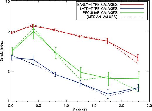
Evolution of the mean Sérsic index values over redshift according the visual classifications of the galaxies within our sample (see also Table 1). Data points for early types and peculiars are slightly offset for the sake of clarity. Dashed lines are similar but taking median values instead. Errors bars are the uncertainty of the mean (|$\sigma /\sqrt{(N-1)}$|, being σ the standard deviation and N the total number of galaxies for each bin). They are slightly larger at 0.2 < z < 0.6 because of the comparatively poor statistics at this redshift interval. From that epoch to higher redshifts there is a clear separation between early-type massive galaxies and the rest of visual types, being all the average Sérsic indices lower at increasing redshift.
Again, our simulations were conducted for exploring potential observational artefacts. By means of comparing Figs 4 and 5, one can check that the trend we observe towards lower Sérsic indices at higher redshifts is maintained with and without corrections. In fact, these corrections are minor. The only noticeable variation would be in the GNS early types mean Sérsic index value in Table 1, which would grow up from 2.73 ± 0.96 to 3.15 ± 1.26. However, cosmic variance may partly be responsible for changing these numbers, as the GNS area (even though it was optimized for increasing the observed number of massive galaxies) is significantly smaller than the EGS POWIR/DEEP2 observations. Finally, in relation to the distribution of the Sérsic indices in Fig. 4 for the galaxies we classified as interacting or irregulars, we see a larger spread. We discuss and interpret the Sérsic index evolution for all our sample in the next section.
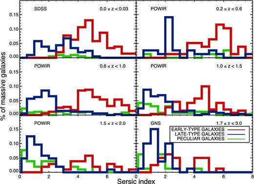
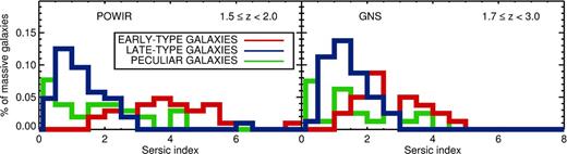
Sérsic index distribution of massive (M* ≥ 1011 h− 270 M⊙) galaxies at different redshift intervals. The Sérsic indices of the individual galaxies have been corrected following the simulations presented in Trujillo et al. (2007; POWIR) and the appendix of this paper (GNS). Colour coding is related with visual morphology: blue for late-type galaxies, red for early-type galaxies and green for peculiar (irregulars/mergers) galaxies. It is pertinent to note that the sharp peak for late-type objects at 0.2 < z < 0.6 is due to the small number statistics for this class of massive galaxies at this redshift interval (see Table 1). For our SDSS sample, the Sérsic indices of discy objects are mainly located in the range of 1 < n < 3 but for some galaxies extend up to n = 5. Conversely, the Sérsic index of spheroid galaxies starts at n ∼ 3 and then peaks at n ∼ 5. This situation differs from our high-z results, where the very high Sérsic indices have disappeared, and on average the values become smaller for all kinds of massive galaxies.
These are the highest redshift histograms of Fig. 4, showing the observed Sérsic index values, without any a posteriori correction based on Trujillo et al. (2007) or our current GNS simulations (Appendix A). The more noticeable change is seen for the GNS data, where it is very conspicuous the non-existence of any large (n > 4.62) Sérsic index. The difference between these histograms and the ones presented in Fig. 4 is small.
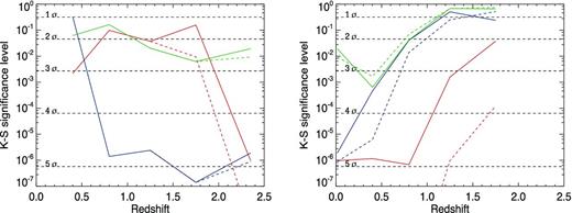
Kolmogorov–Smirnov significance levels comparing the SDSS local sample Sérsic index distribution with all the other redshift bins (left-hand panel) and the GNS highest redshift bin Sérsic index distribution against the rest of the distributions (right-hand panel). The colour coding is the same as in the previous figures: red is for early-type galaxies, blue is for late-type galaxies and green is for peculiar galaxies. Dashed lines represent the same results but without taking into account the corrections for Sérsic indices inferred from our simulations. The reason why dashed lines encompass the whole plot in the right-hand panel is that the last distribution (GNS) is available with and without corrections, but this does not occur for the local SDSS sample. The general trends show that, within our uncertainties, the distributions are diverging from the local relation (left-hand panel) or progressively converging up to the highest redshift bin (right-hand panel). The distributions with the Sérsic indices corrected according to our simulations show a lower departure with respect to the fiducial distribution, but still a significant one.
4 THE OVERALL CHANGE IN THE MASSIVE GALAXY POPULATION WITH REDSHIFT
Many studies (e.g. Shen et al. 2003; Barden et al. 2005; McIntosh et al. 2005; Trujillo et al. 2006) have used n = 2.5 as a quantitative way to segregate between early- and late-type galaxies. We explore, using this criteria, how the percentages of the different types of massive galaxies evolve with redshift. This is shown in Fig. 7(a). This figure clearly indicates that the fraction of massive galaxies with lower Sérsic index values has dramatically increased at higher redshift. If the association between the Sérsic index and the global morphological type that holds at low redshift also applies at high z, this would imply that massive galaxies at the high-z universe were mostly late-type (disc) galaxies. However, there is no guarantee that such an association holds at all redshifts. For this reason, we explore the evolution of the fraction of different galaxy types with redshift using the visual morphologies (see Fig. 7 b). We find that the population of visually classified massive disc galaxies remains almost constant with redshift with perhaps a slight (if any) increase. The most dramatic changes are associated with the early-type and irregular/mergers classes. The fraction of visually classified E/S0 galaxies increased by a factor of 3 since z ∼ 3 to now, whereas a reverse situation is seen for the irregular/merging galaxies. This latter fact agrees with merging becoming more important in massive galaxy evolution at increasing redshift (Bluck et al. 2009, 2012; Conselice, Yang & Bluck 2009; López-Sanjuan et al. 2012). At z ∼ 2.5, late-type and peculiar objects account for the majority of massive galaxies. One of the most important outcomes of Fig. 7 is that the E/S0 type has been the dominant morphological fraction of massive galaxies only since z ∼ 1.
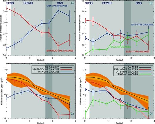
Panel (A): fraction of massive (M* ≥ 1011 h− 270 M⊙) galaxies showing disc-like surface brightness profiles (n < 2.5) and spheroid-like ones (n > 2.5) as a function of redshift. Different colour backgrounds indicate the redshift range expanded for each survey: SDSS, POWIR/DEEP2 and GNS. Error bars are estimated following a binomial distribution. Sérsic indices are corrected based on our simulations (Trujillo et al. 2007, and Appendix A in this paper). Panel (B): same as panel (A) but segregating the massive galaxies according to their visual morphological classification. Blue colour represents late-type (S) objects and red colour represents early-type (E+S0) galaxies, while peculiar (ongoing mergers and irregulars) galaxies are tagged in green. Panel (C): comoving number density evolution of massive galaxies splitted depending on the Sérsic index value. The solid black line corresponds to the total number densities (the sum of the different components), with yellow and orange contours indicating 1σ and 3σ uncertainties in their calculation. Panel (D): same as panel (C) but segregating the massive galaxies according to their visual morphological type.
The number density of massive galaxies has significantly changed since z ∼ 3 (e.g. Rudnick et al. 2003; Pérez-González et al. 2008a; Conselice et al. 2011; Mortlock et al. 2011) with a continuous increase in the number of these objects in the last ∼11 Gyr. In order to probe the emergence of the different galaxy types explored in this paper we have estimated the comoving number density evolution of each class. To do this, we have used the Schechter fits to the stellar mass functions spanning from low to high redshift provided in a series of works: Pérez-González et al. (2008a) (0 < z < 3), Cole et al. (2001) (z = 0), Ilbert et al. (2010) (0.2 < z < 2), Kajisawa et al. (2009) [using the galaxev library (from BC03) alone and in combination with the eazy code (Brammer, van Dokkum & Coppi 2008); 0.5 < z < 3] and Marchesini et al. (2009) (1.3 < z < 3.0). All the mass functions utilized have been derived using BC03 models and normalized to our Chabrier IMF when necessary to be consistent with our data. We have integrated these functions for all massive objects with Mstellar ≥ 1011 h− 270 M⊙. The total number density for massive galaxies appears in Figs 7(c) and (d) as the black line. The yellow and orange backgrounds correspond to its 1σ and 3σ uncertainties. We have later multiplied those numbers by the fractions we have estimated for the different classes of galaxies explored in this work. We show the comoving number density evolution in Figs 7(c) and (d), and the data are tabulated in Table 3. The number density of both disc-like and spheroid-like massive galaxies, according to their Sérsic index, has changed with time. This evolution is particularly significant for spheroid-like objects which are now a factor of ∼10 more numerous per unit volume than at z ∼ 2. About visual morphologies, the number of massive late-type galaxies has also increased as cosmic time progresses, but at a lower rate than early-type galaxies. Finally, the comoving number density of massive irregular/merging galaxies has grown only very mildly, ifat all, in the last ∼11 Gyr.
Comoving number densities for massive (M* ≥ 1011 h− 270 M⊙) galaxies (in 10− 5 h370 Mpc−3 units).
| Redshift | Φtotal | Φn < 2 | Φn > 2 | Φlate | Φearly | Φpeculiar |
|---|---|---|---|---|---|---|
| 0.03 | 50.07 ± 4.21 | 7.01 ± 1.21 | 43.06 ± 3.77 | 16.21 ± 1.84 | 32.17 ± 2.99 | 1.69 ± 0.63 |
| 0.35 | 48.67 ± 9.03 | 9.98 ± 3.18 | 38.69 ± 7.63 | 12.17 ± 3.55 | 30.42 ± 6.38 | 6.08 ± 2.57 |
| 0.65 | 42.89 ± 8.16 | 11.90 ± 2.51 | 30.99 ± 5.99 | 14.00 ± 2.90 | 23.93 ± 4.71 | 4.97 ± 1.31 |
| 0.95 | 34.45 ± 4.34 | 14.14 ± 1.92 | 20.31 ± 2.66 | 14.00 ± 1.93 | 16.31 ± 2.20 | 4.14 ± 0.80 |
| 1.25 | 20.30 ± 1.30 | 10.28 ± 0.87 | 10.02 ± 0.86 | 7.16 ± 0.78 | 7.43 ± 0.80 | 5.70 ± 0.72 |
| 1.55 | 14.62 ± 1.67 | 8.58 ± 1.12 | 6.04 ± 0.88 | 5.94 ± 0.90 | 5.30 ± 0.85 | 3.37 ± 0.67 |
| 1.85 | 11.52 ± 0.62 | 6.65 ± 0.67 | 4.87 ± 0.62 | 4.21 ± 0.66 | 3.32 ± 0.63 | 3.99 ± 0.65 |
| 2.25 | 8.16 ± 0.78 | 6.70 ± 0.77 | 1.46 ± 0.44 | 3.14 ± 0.59 | 2.93 ± 0.58 | 2.09 ± 0.52 |
| 2.75 | 5.30 ± 1.07 | 3.78 ± 0.86 | 1.51 ± 0.50 | 2.27 ± 0.64 | 1.01 ± 0.45 | 2.02 ± 0.60 |
5 DISCUSSION
The evidence collected in the previous section suggests that there is a strong evolution in the morphological properties (both quantitative and qualitative) of the massive galaxy population over time. At high redshift, in agreement with the theoretical expectation, the dominant morphological classes of galaxies are late types and peculiars. Consequently, the morphological and structural types of the majority of the massive galaxies at a given epoch have dramatically evolved as cosmic time increases.
Two effects could play a role towards explaining this significant change of the dominant morphological class. On one hand, the galaxies that are progressively been added into the family of massive objects (i.e. by the merging of less massive galaxies) are incorporated with already spheroidal morphologies. On the other hand, the already old massive galaxies can also evolve towards spheroidal morphologies due to frequent mergers. For instance, frequent minor mergers (Kaviraj 2010; López-Sanjuan et al. 2010; López-Sanjuan et al. 2011; Bluck et al. 2012) with the massive galaxy population may destroy existing stellar discs, and also would be responsible for the appearance of long tails in their luminosity profiles. This scenario could explain why the evolution towards spheroid-like morphologies is stronger when we use the Sérsic index n instead of the visual classification.
In fact, the surface brightness of nearby massive ellipticals is well described with large Sérsic indices due to their bright outer envelopes. These wings, however, seem to disappear at higher and higher redshifts (see Table 1 or Fig. 3) just leaving the inner (core) region of the massive galaxies (Bezanson et al. 2009; Hopkins et al. 2009; Carrasco, Conselice & Trujillo 2010; van Dokkum et al. 2010). The disappearance of these outer envelopes is also connected with the dramatic size evolution reported in previous works (see e.g. Trujillo et al. 2007; Buitrago et al. 2008; Van Dokkum et al. 2010; Trujillo, Ferreras & De la Rosa 2011; McLure et al. 2012). Consequently, it is not only that the typical morphology of the massive galaxy population is changing with redshift, but also that there is a progressive build-up of their outer envelopes, making the morphological evolution appears more dramatic when we use the Sérsic index instead of the visual classification as a morphological segregator.
An open question is whether we are also witnessing the progressive development of bulges with redshift. There are many indications which tell us that this evolution is taking place. For instance Azzollini, Beckman & Trujillo (2009) investigated the luminosity profiles of massive (M* > 1010 M⊙ in this case) discs at 0 < z < 1. Some of these galaxies clearly show an excess of light in their surface brightness profiles in the reddest band which was not present for the bluest. Complementary, Domínguez-Palmero & Balcells (2008) reported nuclear star formation must lead to bulge growth within discs for HST ACS observations in a similar redshift range. However, we noticed there is a lack of studies focusing on the bulge growth with redshift, and its impact in the observed galaxy Sérsic index.
If we were just using the information contained in the change of the fraction of morphological types with redshift, we would be tempted to explain the morphological evolution as being just a consequence of a transformation from one class to another; however, the evolution in the number density of all the classes suggests a more complex scenario. In fact, one of the results we can conclude from the evolution of the number densities of all the massive galaxy classes is that high-z massive disc-like galaxies cannot be the only progenitors of present-day massive spheroid-like galaxies. They are just simply not enough in number to explain the large increase of the number density of elliptical galaxies at low redshifts.
All the morphological classes, maybe with the exception of irregular/merging galaxies, have increased their number densities with cosmic time. These irregular/merging galaxies also have shorter structural lifespans than the other types, and therefore the galaxies in this class must be replenished through time. This emergence of massive galaxies is more efficient (by a factor of ∼2) at creating spheroid-like galaxies than disc-like objects from z ∼ 1 to now (see Fig. 7). The reason why the formation of elliptical galaxies is more efficient at recent times than it was in the past is possibly linked to the lower availability of gas during mergers creating new galaxies (Khochfar & Silk 2006, 2009; Eliche-Moral et al. 2010; Shankar et al. 2011), and thus more likely to contain denser and more concentrated light profiles (Bluck et al. 2012).
It has been reported lately that, apart from the increasing number density of massive galaxies with redshift, the number density of quiescent galaxies among them has risen by a factor of 5 or even more (Barro et al. 2012; Brammer et al. 2011; Cassata et al. 2011; Bell et al. 2012). There is evidence about this quiescence is correlated with the Sérsic index at all redshifts (Bell et al. 2012). This is in perfect agreement with our results, as we undoubtedly observe an increment of the Sérsic index amid our sample towards low z. Moreover, it is reasonable to expect that the level of star formation must have an impact not only in the Sérsic index but also in the galaxy morphology. Following the argument in favour of the appearance of massive and passive galaxies with cosmic time, it is nonetheless difficult to explain why the number densities of late-type massive galaxies slightly rise with redshift. However, we could reconcile the apparently contradictory facts by advocating the large number of passive discs found at high z (McGrath et al. 2008; Messias et al., in preparation). As stated in McLure et al. (2012), this reflects that different mechanisms may account for the quenching of star formation and the morphological transformation of massive galaxies.
If the increment of the Sérsic index with time/redshift (and thus the prominence of bulge and outer envelopes) is linked with the availability of minor companions that will eventually merge with the main galaxy, then spheroid-like massive galaxies must have on average more of them, as it has been observationally confirmed (Mármol-Queraltó et al. 2012). This satellite infalling would explain why these early-type/spheroid-like massive galaxies are not completely devoid of star formation (Pérez-González et al. 2008b; Cava et al. 2010; Bauer et al. 2011; Viero et al. 2012). The risen of massive early-type galaxies appears to be a natural consequence of galaxy mass assembly. The contribution of the various physical mechanisms on changing the galaxy morphology and the existence of a considerable fraction of massive late-type galaxies at low z still challenge our vision of the nature of massive galaxies.
6 SUMMARY
Using a large compilation of massive (M ≥ 1011 h− 270 M⊙) galaxies (∼1100 objects) since z ∼ 3 we have addressed the issue of the morphological change of this population with time. We have found that there is a profound transformation in the morphological content of massive galaxies during this cosmic interval. Massive galaxies were typically disc-like in shape at z ≳ 1 and early-type galaxies have been only the predominant massive class since that epoch. The fraction of early-type morphologies in massive galaxies has changed from ∼20–30 per cent at z ∼ 3 to ∼70 per cent at z = 0 (see Fig. 7).
We have addressed the morphological transformation of the massive galaxies using a quantitative approach, based on Sérsic fits to the surface brightness distribution of the galaxies, and a qualitative approach based on visual classifications. Both analyses agree on a clear morphological change in the dominant morphological class with time. In particular, the quantitative approach, which uses the Sérsic index as a morphological segregator, shows that the number of galaxies with low Sérsic index at high z was higher than in the present-day universe. We interpret this as a consequence of two phenomena: a decrease in the number of early-type galaxies at higher redshift plus an intrinsic decrease of the Sérsic index values of those massive galaxies at earlier cosmic times due to the loss of their extended envelopes.
This paper would have not been possible without hospitality of the IAC, in particular that of Ignacio Trujillo and Jesús Falcón-Barroso. We gratefully thank the contribution of the anonymous referee who helped our scientific discussion, and our editor Keith T. Smith who promptly answered all our requests. We acknowledge the help of Jesús Varela on finding the necessary information of the SDSS sample, Judit Bakos for assistance with SDSS imaging and sky subtraction and also Juan E. Betancort and Inés Flores-Cacho for their scientific feedback, apart from the contributions from the GNS team. We gratefully thank Steven Bamford, Nathan Bourne, Carlos López-Sanjuan and Pablo Pérez-González for useful discussions. This work has been supported by the STFC, NASA through NASA/STScI grant HST-GO11082, the Leverhulme Trust, and the Programa Nacional de Astronomía y Astrofísica of the Spanish Ministry of Science and Innovation under grant AYA2010-21322-C03-02.
Scottish Universities Physics Alliance
REFERENCES
APPENDIX A: GOODS NICMOS SURVEY MASSIVE GALAXIES SIMULATIONS
Images of every mock galaxy were created placing these objects randomly in the GNS pointings. We placed a mock galaxy on each GNS pointing for every simulation in order to avoid altering the typical density (i.e. the number of neighbour galaxies) of the GNS imaging. Each model galaxy (i.e. the 2D surface brightness distribution following the Sérsic function) was convolved with a representative PSF. Specifically we used one of the five natural stars which were utilized in Buitrago et al. (2008). To obtain errors in the same way as in that paper, we also ran galfit using these five different stars and then taking the mean values.
We have identified that the main source of uncertainty in the NICMOS data is the change of the PSF among the different pointings. To illustrate how this affects the recovery of the structural parameters we first present in Figs A1 and A2 how our parameters are recovered when we use the same PSF for creating and recovering the mock galaxies. In Figs A3 and A4, we show the effects on the parameters when we compare the input values with the average values obtained using the five different PSFs.
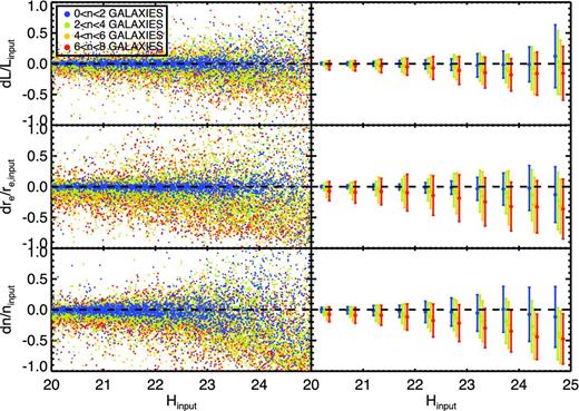
Relative errors – (output-input)/input – of the structural parameters (magnitude, effective radius and Sérsic index) of our simulated GNS galaxies. The right-hand column shows the means in bins of 0.5 mag (with a 5σ outlier-resistant determination), being the error bars the standard deviation of the sample. The information in this plot is tabulated in Table A1.
Relative errors (per cent) and standard deviations on the structural parameters depending on the apparent magnitude (see Fig. A1).
| 0 < n < 2 | 2 < n < 4 | 4 < n < 6 | 6 < n < 8 | |
|---|---|---|---|---|
| 20.0 < HAB, input (mag) < 20.5 | ||||
| δL/L | 0.39 ± 1.75 | −0.53 ± 3.21 | −1.85 ± 6.24 | −2.62 ± 7.36 |
| δre/re | 0.09 ± 2.03 | −1.16 ± 5.27 | −4.63 ± 12.35 | −7.19 ± 15.54 |
| δn/n | −0.34 ± 4.08 | −3.22 ± 6.20 | −6.25 ± 10.59 | −7.62 ± 12.07 |
| 20.5 < HAB, input (mag) < 21.0 | ||||
| δL/L | 0.21 ± 2.61 | −0.99 ± 5.46 | −2.95 ± 7.61 | −3.43 ± 8.20 |
| δre/re | 0.01 ± 2.98 | −2.33 ± 8.31 | −6.78 ± 14.35 | −9.16 ± 17.30 |
| δn/n | −0.97 ± 5.63 | −3.51 ± 8.48 | −7.69 ± 11.25 | −9.13 ± 12.68 |
| 21.0 < HAB, input (mag) < 21.5 | ||||
| δL/L | −0.12 ± 3.85 | −1.34 ± 6.93 | −2.60 ± 10.14 | −3.62 ± 10.74 |
| δre/re | −0.40 ± 4.58 | −2.81 ± 11.39 | −5.08 ± 20.67 | −7.85 ± 21.32 |
| δn/n | −1.42 ± 8.21 | −5.65 ± 12.94 | −7.72 ± 15.04 | −9.08 ± 16.12 |
| 21.5 < HAB, input (mag) < 22.0 | ||||
| δL/L | −0.05 ± 5.17 | −2.56 ± 10.93 | −3.76 ± 13.39 | −4.95 ± 13.55 |
| δre/re | −0.50 ± 4.79 | −4.98 ± 17.21 | −8.46 ± 25.80 | −9.54 ± 29.76 |
| δn/n | −2.47 ± 9.68 | −6.85 ± 14.97 | −10.83 ± 20.77 | −11.80 ± 21.14 |
| 22.0 < HAB, input (mag) < 22.5 | ||||
| δL/L | −1.03 ± 7.28 | −2.87 ± 12.06 | −5.83 ± 15.87 | −6.79 ± 18.50 |
| δre/re | −1.70 ± 8.48 | −5.33 ± 17.56 | −8.22 ± 27.02 | −14.28 ± 32.00 |
| δn/n | −3.55 ± 17.15 | −8.50 ± 19.65 | −11.86 ± 22.91 | −17.65 ± 26.70 |
| 22.5 < HAB, input (mag) < 23.0 | ||||
| δL/L | −1.46 ± 9.27 | −3.40 ± 18.16 | −6.97 ± 19.19 | −11.04 ± 22.58 |
| δre/re | −1.48 ± 10.75 | −5.55 ± 26.98 | −10.61 ± 33.02 | −18.60 ± 37.86 |
| δn/n | −3.74 ± 22.80 | −8.20 ± 25.31 | −13.99 ± 28.88 | −21.90 ± 29.83 |
| 23.0 < HAB, input (mag) < 23.5 | ||||
| δL/L | −2.70 ± 18.92 | −5.54 ± 22.91 | −10.57 ± 22.24 | −14.38 ± 25.00 |
| δre/re | −3.38 ± 18.65 | −7.10 ± 33.57 | −15.11 ± 38.94 | −24.55 ± 39.17 |
| δn/n | −5.29 ± 29.66 | −11.14 ± 34.34 | −18.92 ± 32.87 | −29.79 ± 31.89 |
| 23.5 < HAB, input (mag) < 24.0 | ||||
| δL/L | −1.28 ± 21.90 | −8.12 ± 22.41 | −11.57 ± 26.88 | −17.93 ± 26.23 |
| δre/re | −3.81 ± 26.00 | −10.21 ± 33.56 | −17.86 ± 43.47 | −32.17 ± 39.63 |
| δn/n | 0.61 ± 37.18 | −18.35 ± 36.38 | −24.90 ± 37.94 | −35.02 ± 33.59 |
| 24.0 < HAB, input (mag) < 24.5 | ||||
| δL/L | −0.99 ± 28.30 | −7.27 ± 34.80 | −16.06 ± 33.78 | −15.98 ± 34.87 |
| δre/re | −2.13 ± 36.39 | −13.48 ± 41.48 | −29.16 ± 44.22 | −32.70 ± 42.43 |
| δn/n | −7.57 ± 43.98 | −27.35 ± 41.82 | −39.53 ± 40.77 | −44.10 ± 36.75 |
| 24.5 < HAB, input (mag) < 25.0 | ||||
| δL/L | 12.20 ± 51.04 | 2.50 ± 51.58 | −5.73 ± 44.09 | −15.50 ± 43.68 |
| δre/re | −12.85 ± 45.18 | −22.74 ± 46.45 | −31.77 ± 43.55 | −36.15 ± 48.64 |
| δn/n | −11.73 ± 49.37 | −38.99 ± 42.35 | −44.67 ± 42.69 | −47.58 ± 40.68 |
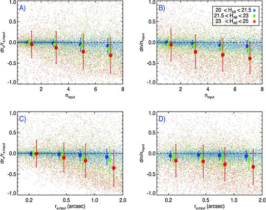
Relative errors – (output-input)/input – of the effective radius (first column) and the Sérsic index (second column) as a function of the input Sérsic index (first row) and the input effective radius (second row). Galaxies are coloured according to their magnitude. For the sake of clarity, mean values (derived with a 5σ outlier-resistant determination) were added using four intervals in effective radius and Sérsic index, with the error bars being their standard deviation. Sérsic index intervals are 0 < n < 2, 2 < n < 4, 4 < n < 6 and 6 < n < 8. Effective radius intervals are 0.15 < re < 0.3 arcsec, 0.3 < re < 0.6 arcsec, 0.6 < re < 0.9 arcsec and 0.9 < re < 2 arcsec. Note that the colour of these mean points is the same as the one of the galaxy individual points. The information in this plot is tabulated in Table A2.
Relative errors (per cent) and standard deviations on the structural parameters (see Fig. A2)
| δre/re | 20 < HAB (mag) < 21.5 | 21.5 < HAB (mag) < 23 | 23 < HAB (mag) < 25 |
|---|---|---|---|
| 0 < n < 2 | −0.04 ± 3.09 | −1.00 ± 7.97 | −4.89 ± 31.91 |
| 2 < n < 4 | −2.14 ± 8.27 | −5.13 ± 20.61 | −12.66 ± 38.79 |
| 4 < n < 6 | −5.71 ± 15.87 | −9.08 ± 28.73 | −22.12 ± 42.84 |
| 6 < n < 8 | −8.16 ± 18.05 | −13.98 ± 33.45 | −31.04 ± 42.55 |
| 0.15 < re (arcsec) < 0.3 | −0.94 ± 5.45 | 0.05 ± 13.79 | −0.87 ± 32.27 |
| 0.3 < re (arcsec) < 0.6 | −2.28 ± 9.02 | −2.71 ± 20.11 | −10.47 ± 35.21 |
| 0.6 < re (arcsec) < 0.9 | −4.15 ± 12.67 | −9.55 ± 24.26 | −17.50 ± 40.12 |
| 0.9 < re (arcsec) < 2.0 | −8.44 ± 18.68 | −15.66 ± 32.69 | −35.02 ± 43.53 |
| δn/n | 20 < HAB < 21.5 | 21.5 < HAB < 23 | 23 < HAB < 25 |
| 0 < n < 2 | −0.84 ± 6.23 | −3.57 ± 16.86 | −5.51 ± 39.42 |
| 2 < n < 4 | −3.75 ± 8.71 | −7.83 ± 20.63 | −22.65 ± 39.74 |
| 4 < n < 6 | −7.08 ± 12.33 | −12.19 ± 24.38 | −30.01 ± 39.47 |
| 6 < n < 8 | −8.85 ± 14.25 | −16.94 ± 26.32 | −38.55 ± 36.30 |
| 0.15 < re (arcsec) < 0.3 | −5.99 ± 12.04 | −7.56 ± 22.54 | −17.43 ± 39.18 |
| 0.3 < re (arcsec) < 0.6 | −3.93 ± 10.03 | −7.20 ± 21.14 | −19.31 ± 38.89 |
| 0.6 < re (arcsec) < 0.9 | −5.08 ± 11.05 | −11.31 ± 21.56 | −26.36 ± 39.79 |
| 0.9 < re (arcsec) < 2.0 | −6.38 ± 12.51 | −13.74 ± 25.47 | −32.49 ± 41.78 |


In Figs A1 and A3, we show the relationship between the relative errors in the structural parameters (magnitude, effective radius and Sérsic index) versus the galaxy input magnitude. The relative errors are calculated as (output-input)/input (i.e. a negative per cent refer to cases where the output is smaller than the input and vice versa). The left-hand column of the plot displays the structural parameters of individual mock galaxies, whereas the right-hand column shows their means in bins of 0.5 mag. The mean values of the structural parameters were derived using a robust method which removes the 5σ outliers. Error bars represent the standard deviation of the sample. To appreciate how the effect on the structural parameter is linked to the input Sérsic index of the mock galaxies we split the sample into four groups (0 < n < 2, 2 < n < 4, 4 < n < 6 and 6 < n < 8). The results shown in Fig. A3 are tabulated in Table A3. At increasing Sérsic index values, the recovery of the structural parameters is more affected. We note that galaxies with low Sérsic index are well recovered down to our faintest magnitude. An average galaxy in our GNS sample (H = 22.5 mag) with an input Sérsic index of n = 4 will have its effective radius biased only by a ∼10 per cent and its Sérsic index around ∼20 per cent.
Relative errors (per cent) and standard deviations on the structural parameters depending on the apparent magnitude using five different PSFs (see Fig. A3).
| 0 < n < 2 | 2 < n < 4 | 4 < n < 6 | 6 < n < 8 | |
|---|---|---|---|---|
| 20.0 < HAB, input (mag) < 20.5 | ||||
| δL/L | −0.15 ± 2.95 | −3.39 ± 5.48 | −9.09 ± 7.90 | −14.50 ± 8.47 |
| δre/re | 0.79 ± 5.25 | −4.95 ± 9.28 | −14.69 ± 14.79 | −26.56 ± 16.21 |
| δn/n | −4.39 ± 10.97 | −13.84 ± 16.60 | −24.76 ± 19.20 | −36.22 ± 19.58 |
| 20.5 < HAB, input (mag) < 21.0 | ||||
| δL/L | −0.14 ± 3.82 | −3.44 ± 6.32 | −9.31 ± 9.39 | −15.08 ± 9.23 |
| δre/re | 0.20 ± 5.36 | −4.57 ± 10.89 | −16.51 ± 16.28 | −26.97 ± 17.87 |
| δn/n | −4.16 ± 11.25 | −13.82 ± 17.91 | −23.84 ± 19.20 | −38.19 ± 19.64 |
| 21.0 < HAB, input (mag) < 21.5 | ||||
| δL/L | −0.57 ± 4.92 | −3.68 ± 7.55 | −9.49 ± 9.25 | −14.29 ± 10.06 |
| δre/re | −0.86 ± 7.00 | −5.73 ± 13.66 | −16.66 ± 18.67 | −26.05 ± 18.35 |
| δn/n | −5.76 ± 12.02 | −15.86 ± 17.54 | −26.63 ± 20.50 | −36.08 ± 19.52 |
| 21.5 < HAB, input (mag) < 22.0 | ||||
| δL/L | −0.49 ± 5.53 | −4.59 ± 10.36 | −9.94 ± 12.10 | −14.68 ± 11.82 |
| δre/re | −0.29 ± 7.33 | −7.05 ± 17.72 | −17.91 ± 22.02 | −25.85 ± 24.09 |
| δn/n | −6.04 ± 13.43 | −16.61 ± 18.69 | −27.84 ± 22.26 | −36.30 ± 22.71 |
| 22.0 < HAB, input (mag) < 22.5 | ||||
| δL/L | −1.47 ± 7.60 | −4.71 ± 13.41 | −11.55 ± 13.82 | −14.61 ± 15.32 |
| δre/re | −1.75 ± 9.51 | −7.38 ± 19.43 | −16.97 ± 25.13 | −26.68 ± 26.94 |
| δn/n | −8.18 ± 17.99 | −18.82 ± 21.73 | −28.87 ± 22.24 | −39.18 ± 24.90 |
| 22.5 < HAB, input (mag) < 23.0 | ||||
| δL/L | −1.67 ± 10.03 | −5.89 ± 16.50 | −11.89 ± 18.38 | −17.96 ± 21.49 |
| δre/re | −1.28 ± 11.40 | −9.24 ± 26.02 | −17.99 ± 29.22 | −27.32 ± 34.57 |
| δn/n | −8.25 ± 22.92 | −18.29 ± 26.96 | −29.25 ± 27.00 | −41.66 ± 26.64 |
| 23.0 < HAB, input (mag) < 23.5 | ||||
| δL/L | −3.80 ± 19.13 | −7.12 ± 22.24 | −14.63 ± 19.75 | −16.61 ± 24.12 |
| δre/re | −2.84 ± 21.33 | −10.78 ± 32.29 | −20.79 ± 34.39 | −25.78 ± 39.19 |
| δn/n | −7.49 ± 29.62 | −20.09 ± 33.28 | −32.47 ± 31.11 | −42.58 ± 29.90 |
| 23.5 < HAB, input (mag) < 24.0 | ||||
| δL/L | −1.89 ± 22.85 | −10.19 ± 22.94 | −14.19 ± 25.32 | −20.52 ± 24.32 |
| δre/re | −2.21 ± 27.87 | −11.57 ± 35.12 | −20.76 ± 39.58 | −31.83 ± 41.51 |
| δn/n | −3.87 ± 38.56 | −24.95 ± 36.87 | −36.53 ± 34.02 | −46.46 ± 31.09 |
| 24.0 < HAB, input (mag) < 24.5 | ||||
| δL/L | −1.50 ± 25.40 | −10.23 ± 32.27 | −16.10 ± 34.15 | −16.71 ± 36.33 |
| δre/re | −3.60 ± 35.90 | −14.78 ± 43.22 | −30.37 ± 42.96 | −30.21 ± 45.39 |
| δn/n | −10.32 ± 42.23 | −32.03 ± 42.13 | −47.21 ± 38.40 | −51.98 ± 36.24 |
| 24.5 < HAB, input (mag) < 25.0 | ||||
| δL/L | 3.48 ± 38.67 | −0.99 ± 47.79 | −7.13 ± 48.32 | −17.63 ± 39.12 |
| δre/re | −11.83 ± 45.10 | −24.02 ± 44.12 | −33.58 ± 47.25 | −36.64 ± 47.00 |
| δn/n | −17.46 ± 48.50 | −42.41 ± 46.73 | −45.35 ± 44.40 | −53.14 ± 39.50 |
In addition to the dependence of the apparent magnitude of the objects on recovering their structural parameters, in Figs A2 and A4 we explore what is the effect of the size (lower row) and intrinsic shape (upper row) for this matter. Galaxies are colour coded in these figures according to their magnitude. Combining the information contained in Figs A3 and A4, we find that the key parameters for retrieving accurate structural parameters are the apparent magnitude and the Sérsic index. The effective radius of the objects play a minor role. The results shown in Fig. A4 are tabulated in Table A4.
Relative errors (per cent) and standard deviations on the structural parameters using five different PSFs (see Fig. A4).
| δre/re | 20 < HAB (mag) < 21.5 | 21.5 < HAB (mag) < 23 | 23 < HAB (mag) < 25 |
|---|---|---|---|
| 0 < n < 2 | 0.06 ± 5.77 | −1.16 ± 9.59 | −4.66 ± 32.39 |
| 2 < n < 4 | −5.12 ± 11.07 | −8.03 ± 21.95 | −14.81 ± 38.86 |
| 4 < n < 6 | −15.72 ± 16.22 | −17.63 ± 25.57 | −25.64 ± 41.12 |
| 6 < n < 8 | −26.47 ± 17.73 | −26.40 ± 29.20 | −30.86 ± 43.40 |
| 0.15 < re (arcsec) < 0.3 | −4.88 ± 13.91 | −2.74 ± 16.53 | −0.63 ± 31.95 |
| 0.3 < re (arcsec) < 0.6 | −12.01 ± 15.03 | −10.85 ± 19.95 | −12.85 ± 34.54 |
| 0.6 < re (arcsec) < 0.9 | −14.19 ± 17.17 | −16.98 ± 24.64 | −19.68 ± 40.32 |
| 0.9 < re (arcsec) < 2.0 | −17.15 ± 21.19 | −21.85 ± 30.48 | −37.75 ± 43.51 |
| δn/n | 20 < HAB < 21.5 | 21.5 < HAB < 23 | 23 < HAB < 25 |
| 0 < n < 2 | −4.89 ± 11.68 | −7.60 ± 18.65 | −9.07 ± 39.19 |
| 2 < n < 4 | −14.57 ± 17.28 | −17.79 ± 22.82 | −29.09 ± 40.43 |
| 4 < n < 6 | −25.06 ± 19.75 | −28.64 ± 23.92 | −39.53 ± 37.22 |
| 6 < n < 8 | −36.86 ± 19.70 | −39.00 ± 24.87 | −48.32 ± 34.49 |
| 0.15 < re (arcsec) < 0.3 | −37.61 ± 22.17 | −37.41 ± 24.34 | −35.55 ± 39.30 |
| 0.3 < re (arcsec) < 0.6 | −21.64 ± 20.35 | −22.08 ± 24.19 | −29.12 ± 39.11 |
| 0.6 < re (arcsec) < 0.9 | −16.58 ± 18.55 | −19.83 ± 23.63 | −29.86 ± 40.01 |
| 0.9 < re (arcsec) < 2.0 | −13.81 ± 17.93 | −19.11 ± 25.80 | −35.62 ± 42.06 |
The most interested output of our tests using the mean value from the fits of different PSFs is that the size of the source plays now a fundamental role at characterizing the error on the structural parameters. As expected, large sources are less affected by changes in the PSF and the bias on the structural parameters remains basically the same as when we use just a single PSFs. However, at smaller sizes the effect of not knowing accurately the PSF at the source implies that the Sérsic index uncertainty is large, although sizes are retrieved accurately. Summarizing, neither any effect nor combination of effects is large enough to modify the main results of this paper. Moreover, as stated on the main text of this paper, we use these simulations to correct, based on the observed (output) apparent magnitude, effective radius and Sérsic index, the structural parameters presented in this work.
SUPPORTING INFORMATION
Additional Supporting Information may be found in the online version of this paper.
Table S1. Structural parameters from our massive (M⋆ > 1011h− 270M⊙) SDSS (z < 0.03) galaxy sample (Supplementary Data).
Please note: Oxford University Press are not responsible for the content or functionality of any supporting materials supplied by the authors. Any queries (other than missing material) should be directed to the corresponding author for the article.
