


Abstract
Non-thermal motions in the intracluster medium (ICM) are believed to play a non-negligible role in the pressure support to the total gravitating mass of galaxy clusters. Future X-ray missions, such as ASTRO-H and ATHENA, will eventually allow us to directly detect the signature of these motions from high-resolution spectra of the ICM. In this paper, we present a study on a set of clusters extracted from a cosmological hydrodynamical simulation, devoted to explore the role of non-thermal velocity amplitude in characterizing the cluster state and the relation between observed X-ray properties. In order to reach this goal, we apply the X-ray virtual telescope PHOX to generate synthetic observations of the simulated clusters with both Chandra and ATHENA, the latter used as an example for the performance of very high-resolution X-ray telescopes. From Chandra spectra we extract global properties, e.g. luminosity and temperature, and we accurately estimate the gas velocity dispersion along the line of sight achievable from the broadening of emission lines from heavy ions (e.g. Fe) resolved in ATHENA spectra. Given the good agreement found between simulations (true, intrinsic solution) and mock observations (detectable amplitude of non-thermal velocities), we further extend the analysis to the relation between non-thermal velocity dispersion of the gas and the LX–T scaling law for the simulated clusters. Interestingly, we find a clear dependence of slope and scatter on the selection criterion for the clusters, based on the level of significance of non-thermal motions. Namely, the scatter in the relation is significantly reduced by the exclusion of the clusters, for which we estimate the highest turbulent velocities. Such velocity diagnostics appears therefore as a promising independent way to identify disturbed clusters, in addition to the commonly used morphological inspection.
1 INTRODUCTION
During the mass assembly in galaxy clusters, interactions between subhaloes and merging events can generate substantial streaming motions and turbulence in the hot gas filling the cluster potential well. Additionally, a number of processes taking place in galaxy clusters, especially in the inner regions, are most likely responsible for the transfer of energy from large modes to smaller modes, causing rotation, streaming and, mainly, turbulent motions to establish in the intracluster medium (ICM). Among these physical processes, mergers and sloshing of dark matter (DM) cuspy cores are believed to cause large-scale motions, and in addition the active galactic nucleus (AGN) activity and its interaction with the surrounding gas can cause turbulence in the central region.
Numerically, the non-thermal components of ICM motions have been investigated by means of hydrodynamical simulations of galaxy clusters, which uniquely provide full three-dimensional information on the gas velocity field. The establishment of ICM bulk, streaming and rotational motions during the growth and assembly of simulated galaxy clusters is believed to contribute, especially in the central part of the system, to the cluster pressure support and therefore to the virial estimate of the total mass up to significant fractions (e.g. Pawl, Evrard & Dupke 2005; Fang, Humphrey & Buote 2009; Lau, Kravtsov & Nagai 2009; Biffi, Dolag & Böhringer 2011; Lau et al. 2011). Moreover, several studies on smoothed particle hydrodynamics (SPH) and adaptive mesh refinement (AMR) simulations of cluster-like haloes have addressed the turbulent velocity field in clusters (e.g. see recent work by Paul et al. 2011; Valdarnini 2011; Vazza et al. 2011), estimating the pressure support due to chaotic motions to be of the order of ∼20–30 per cent of the total pressure (e.g. Norman & Bryan 1999; Dolag et al. 2005; Iapichino & Niemeyer 2008; Vazza et al. 2009, 2011; Iapichino et al. 2011). Tighter constraints on the gas velocity field are necessary in order to obtain precise measurements of the total gravitating mass, which is the most important, intrinsic quantity to determine. In particular, the account for non-thermal motions is essential for mass estimates based on X-ray global properties (e.g. gas density and temperature), via the assumption of hydrostatic equilibrium (e.g. Rasia et al. 2006, 2012; Piffaretti & Valdarnini 2008).
The presence of non-thermal motions in the gas velocity field within galaxy clusters is also suggested by several observational evidences, coming from radio observations of polarized synchrotron emission in cluster radio galaxies (e.g. Cassano & Brunetti 2005; Bonafede et al. 2010), measurements of the resonant scattering effects (Churazov et al. 2010; Zhuravleva et al. 2010) and study of the fluctuations in pressure (Schuecker et al. 2004) and surface brightness (Churazov et al. 2012) maps, obtained with X-ray telescopes. However, mainly indirect indications of ICM turbulence have been possible so far. Only with the XMM–Newton Reflection Grating Spectrometer (RGS) spectrometer, weak upper limits have been set on the turbulent velocities in a set of galaxy clusters, as recently discussed in Sanders, Fabian & Smith (2011).
Future X-ray missions, such as ASTRO-H, will allow us to achieve direct estimations of the ICM non-thermal velocities with great accuracy, thanks to the high spectral resolution expected to be reached. In fact, X-ray high-precision spectroscopy potentially offers one of the most promising ways to directly measure such gas motions, detectable from the detailed study of the shape and centroid of resolved spectral emission lines.
Theoretically, the non-thermal component of the gas velocity, along the line of sight (l.o.s.), can be very well constrained by studying the shape of heavy-ion emission lines in the X-ray spectra, for which the broadening can be significantly more sensitive to non-thermal velocities of the gas rather than to thermal motion (e.g. Rebusco et al. 2008). The expectations for such line diagnostics are related in particular to the most prominent emission line in X-ray spectra, namely the ∼6.7 keV line from helium-like iron. In fact, the large atomic mass of the Fe xxv ion significantly reduces the thermal line broadening and the line width turns out to be definitely more sensitive to turbulent gas motions (Inogamov & Sunyaev 2003; Sunyaev, Norman & Bryan 2003).
Here we discuss the prospect of using high-resolution spectra to detect the amplitude of non-thermal gas motions with the aim of characterizing more precisely galaxy clusters and observed relations between their X-ray properties, such as the LX–T scaling relation.
To this scope, we employ a set of numerically simulated clusters, obtained with the TreePM/SPH parallel code p-gadget3 including a large variety of physical processes to describe the baryonic component, and perform X-ray synthetic observations of the haloes with PHOX (Biffi et al. 2012). The paper is structured as follows. First, we will describe the simulated data set of galaxy clusters (Section 2) and the generation of mock X-ray spectra with the Chandra telescope and the X-ray spectrometer originally planned for the ATHENA satellite, as prototype for X-ray spectroscopy at very high energy resolution. In Section 3, we will describe the analysis performed to obtain global properties, such as luminosity and temperature, from the Chandra spectra and to estimate the gas non-thermal velocity dispersion, from the velocity broadening of the iron lines in the high-resolution ATHENA spectra. The analysis on the gas velocity dispersion, calculated directly from the simulation, is presented in Section 4.1. The comparison against the detectable velocities obtained from the synthetic high-resolution spectra is then discussed in Section 4.2. Using the Chandra mock observations, we explore the LX–T scaling relation for the simulated clusters in Section 4.3. In Section 5, we discuss the effects on the best-fitting relation, due to the non-thermal fraction of the ICM motions, and the relation between velocity diagnostics and cluster internal state. Our conclusions are finally summarized in Section 6.
2 THE SAMPLE OF SIMULATED CLUSTERS
The sample of simulated cluster-like haloes analysed here has been extracted from a cosmological hydrodynamical simulation performed with the TreePM/SPH parallel code p-gadget3. In this extended version of gadget-2 (Springel, White & Hernquist 2001; Springel 2005), a vast range of baryonic physics, at a high level of detail, is included, such as cooling, star formation and supernova (SN) driven winds (Springel & Hernquist 2003), chemical enrichment from stellar population, asymptotic giant branch (AGB) stars and SNe (Tornatore et al. 2004, 2007), low-viscosity SPH (Dolag et al. 2005), black hole growth and feedback from AGN (Springel, Di Matteo & Hernquist 2005; Fabjan et al. 2010). The simulated box has a side of 352 h−1 Mpc, in comoving units, resolved with 2 × 5943 particles, which results in a mass resolution of mDM = 1.3 × 10¹⁰ and mgas = 5.2 × 10⁸, for DM and gas particles, respectively. For the simulation, and throughout the following, the cosmology assumed refers to the 7-year WMAP estimates (Komatsu et al. 2011), i.e. Ω0 = 0.268, ΩΛ = 0.728, Ωb = 0.044, σ8 = 0.776 and h = 0.704.
The sample of clusters consists of 43 objects, selected among the most massive haloes in the simulated box, for a snapshot of the simulation at z = 0.213. The selection criterion adopted requires the cluster mass encompassed by R500,1M500, to be >3 × 10¹⁴ h−1 M⊙, at the redshift considered.
3 X-RAY SYNTHETIC OBSERVATIONS
The mock X-ray observations have been performed for the selected haloes of the sample by means of the virtual X-ray simulator PHOX. For a detailed description of the method implemented in PHOX, we refer to Biffi et al. (2012).
3.1 Generation of the virtual photon lists
The snapshot of the hydrodynamical simulation considered, referring to redshift z = 0.213, has been first processed with Unit 1 of PHOX as a whole, generating the virtual photon cube associated with the X-ray-emitting gas component in the simulated cosmic volume.
For all the gas particles, model spectra have been calculated and sampled with packages of photons, each of them in the rest frame of the corresponding emitting particle. The model adopted to calculate each theoretical spectrum was an absorbed, single-temperature VAPEC2 model Smith et al. (2001), implemented in xspec3 (Arnaud 1996). Here, we make use of the parameter within xspec (v.12) to include the thermal broadening of emission lines in the model spectra. Temperature, density and chemical abundances (see Appendix A for details on the implementation of metal composition in PHOX) are obtained directly from the hydrosimulation output. Additionally, we fixed the redshift at the value of the simulated data cube (z = 0.213) and the equivalent hydrogen column density for the WABS absorption model (Morrison & McCammon 1983) to a fiducial value of 1020 cm−2. At the end of this first stage, the photon data base associated with the simulation output contains roughly 107 photon packages (∼109 photons in total), for fiducial values of collecting area and exposure time of 1000 cm2 and 1 Ms, respectively.
With PHOX Unit 2, we then assume to observe the photons from an l.o.s. aligned with the z-axis of the simulation cube and correct photon energies for the Doppler shift due to the emitting-particle motions along this l.o.s.. During this geometrical stage of the process, we also select cylindrical subregions along the l.o.s., corresponding to the 43 selected cluster-like haloes. For each cluster halo, the selected subregion is centred on the centre of mass and encloses the region within R500, in the xy plan, throughout the box depth (along the z-axis). For the time frame considered here and the cosmology used, the luminosity distance between the observer, positioned along the positive z-axis, and the observed region is 1047.6 Mpc, in physical units. Typically, we obtain 1–2 × 10⁶ photons per halo, for 100 ks exposure.
The photon lists produced in this general way are convolved by PHOX with real instrumental responses of Chandra and also for a high-energy resolution response, originally planned for the X-ray spectrometer of ATHENA. The synthetic spectra are fitted by means of the X-ray package xspec v.12.6.0 (Arnaud 1996).
3.2 Chandra synthetic spectra
To create Chandra synthetic spectra, we use the redistribution matrix file (RMF) and ancillary response file (ARF) of the Chandra ACIS-I3 detector aim-point. The field of view (FoV) of Chandra, which is |$17\times 17\,\text{arcmin}^{2}$|, corresponds to a physical scale of 3.52 Mpc per side, for the given cosmology and redshift. This encloses typically the region within 1–1.2R500 for most of the clusters in the sample, except for the seven most massive haloes, for which the Chandra FoV captures a region slightly smaller than the one out to R500. In such cases, however, one can in principle compose a mosaic with multiple Chandra pointings in order to cover the clusters up to R500. Therefore, we convolve the photon lists corresponding to the whole R500 region with the response of Chandra and analyse the corresponding spectra, for all the clusters in the sample.
3.2.1 Temperature and bolometric luminosity
We fit Chandra spectra either with an absorbed, single-temperature or with a two-temperature APEC model, depending on the goodness of the single-temperature fit. The spectra are regrouped requiring a minimum of 10 counts per energy bin. Whenever the spectral fit was still poor, spectra were instead regrouped with a minimum of 20 counts. The absorption is fixed to the fiducial value adopted to generate photons. Given the characteristics of the Chandra response, we assumed the redshift to be fixed at the initial value of the simulation and only temperature, metallicity and normalization were free in the fit.
From the spectral best fit in the 0.5–10 keV range, we directly obtain the temperature of the cluster.4
The total X-ray luminosity, LX, is extrapolated from the best-fitting spectral model out to the entire energy range defined by the ACIS-I3 detector response, to obtain an approximate bolometric luminosity.
3.3 High-resolution synthetic spectra
In the present work, we consider the ideal instrumental response of the spectrometer designed for the ATHENA satellite, which has, however, not been chosen as the next European Space Agency (ESA) L-class mission in the recent mission selection process. Nevertheless, we use this as prototype and goal for next-generation high-resolution X-ray spectrometers (similar to ASTRO-H), fundamental to explore the details of hot plasma emission.
Therefore, the mock spectra are simulated from the ideal photon lists of the 43 haloes in the sample by using the latest response (RSP) matrix planned for the ATHENA X-ray Microcalorimeter Spectrometer (XMS). For the given cosmological parameters and redshift, the small FoV of such instrument (|$2.4\times 2.4\,\text{arcmin}^2$|) encloses a region of 497.52 kpc per side. We centre the FoV on the centre of the cluster, probing therefore the very central part.
3.3.1 Velocity broadening
Given the high-energy resolution provided by the XMS, spectral emission lines are very well resolved. In fact, we restrict the spectral analysis to the observed 5–6.5 keV energy band, containing the iron Kα complex around 6.7 keV (rest-frame energy), and fit with an absorbed BAPEC5 model (see Fig. 1 for an example with one of the presented haloes), i.e. a velocity and thermally broadened emission spectrum for collisionally ionized diffuse gas. The model assumes the distribution of the gas non-thermal velocity along the l.o.s. to be Gaussian and the velocity broadening is quantified by the standard deviation, σ, of this distribution.
4 RESULTS
4.1 Velocity statistics
Our first goal is to investigate the properties of the ICM velocity field in the simulated data directly, in order to establish the level of reliability of the mock data results and therefore the validity of the expectations for high-resolution spectroscopy. Gas particles in the simulated haloes have been selected to reside within R500 in the xy plane, excluding the low-temperature (Tgas < 3 × 10⁴ K) and star-forming (gas particles with >10 per cent of cold fraction) phase of the gas. This selection is done to resemble in the most faithful way possible the X-ray-emitting gas residing in the region observed with the X-ray virtual telescope PHOX. In the following, we will always refer to regions in the xy plane, considering the cylinder-like volume along the l.o.s., aligned with the z-axis of the simulated box.
From Fig. 2, the relation between the value of σ500,m (i.e. weighted by the particle mass) and M500 shows that, in general, more significant motions of the gas are expected in more massive systems. Ideally, the mass-weighted values should trace in the most faithful way the intrinsic quantities characterizing the cluster, since they are closely related to the potential well of the halo. However, X-ray observations of the ICM are more sensitive to the emission properties of the gas, such as the EM,6 and rather provide estimates for an EM-weighted-like velocity dispersion. We therefore investigate the relation between mass- and EM-weighted velocity dispersions, σ500,m and σ500,EM, respectively.
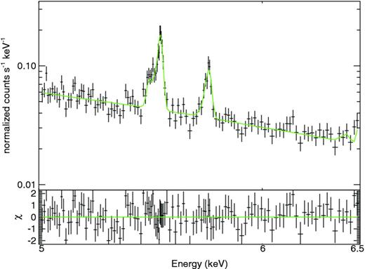
Zoom-in on to the 5–6.5 keV energy band, containing the He- and H-like iron emission lines (at the rest-frame energy ∼6.7 and ∼6.96 keV), from the synthetic ATHENA XMS spectrum of one of the sample clusters. In the figure we show the best-fitting BAPEC model to the data (green curve).
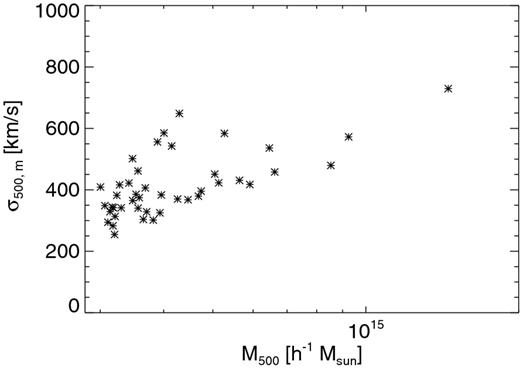
Theoretical value of the mass-weighted velocity dispersion, σm, calculated within R500 (in the plane perpendicular to the l.o.s. direction), reported as a function of the halo mass M500, in h−1 M⊙.
The comparison is shown in Fig. 3, wherein both values of σ500,w are calculated for the gas residing within R500, in the plane perpendicular to the l.o.s.. The relation found between the two definitions of σ500,w is not coincident with the one-to-one relation (overplotted in red in the figure), as the EM-weighted value is likely to be affected by the thermodynamical status of the gas, i.e. by processes such as turbulence, merging and substructures. Despite this, the two values are fairly well correlated.
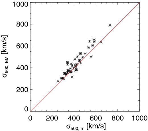
Theoretical value of the EM-weighted velocity dispersion, σ500,EM versus the mass-weighted value, σ500,m, in km s−1. Both values are calculated for the region within R500, in the plane perpendicular to the l.o.s. direction. Overplotted in red is the curve referring to the one-to-one relation.
For the purpose of our following analysis and the comparison against synthetic X-ray data, however, we decide to use the EM-weighted velocity dispersion, σ500,EM, which is more directly related to the X-ray emission of the gas, because of the proportionality between the normalization of the X-ray spectrum and the gas EM itself.
In order to probe the global, dynamical structure of the ICM, we would need to observationally measure the gas velocity dispersion within the whole R500 region. Therefore, we explore the relation between the estimated values of the velocity broadening along the l.o.s. in different regions of the cluster, shown in Fig. 4. It is evident from the figure that the value calculated for the gas within R500 correlates linearly with the value computed in smaller, internal regions, namely for r < 0.3R500 (upper panel) and for the region covered by the FoV of ATHENA, ∼0.15R500 (lower panel). With respect to the one-to-one correlation (red line in Fig. 4), however, outliers are present in this sample, showing that prominent substructures in the velocity field of the gas must be present in the observed regions around the clusters. Here, as in Fig. 2 , deviations can also be related to subhaloes residing in the projected R500, i.e. in the region observed along the l.o.s., but not necessarily comprised within the three-dimensional R500.
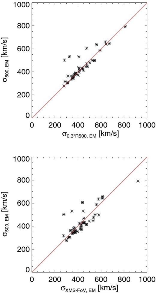
Relation between the EM-weighted velocity dispersion within R500, σ500,EM, and the analogous values calculated for the region within 0.3R500 (top panel) and the region covered by the FoV of ATHENA, (i.e. ∼0.15R500; bottom panel). Overplotted in red is the curve referring to the one-to-one relation.
Therefore, the level of complexity in the spatial structure of the ICM velocity field can be singled out by the comparison between the velocity dispersion calculated in the R500 region and the values corresponding to smaller, inner regions.
Nevertheless, the relations discussed ensure that, for the purposes of this work, we can safely
assume the EM-weighted velocity dispersion instead of the mass-weighted value to trace the intrinsic velocity structure;
focus on the expected value for the whole R500 region of the cluster. This traces fairly well the internal motions also within smaller regions, as those covered by instruments with a smaller FoV, with the exception of those cases where self-bound substructures in the outskirts, or more likely along the l.o.s., are clearly present and might be important to consider.
4.2 Comparison against synthetic data
The ICM velocity dispersion calculated directly from the simulation can here be used to compare against the mock ATHENA data, which is the prototype for the high-resolution spectroscopy (XMS) required to measure the gas velocity dispersion along the l.o.s. from resolved emission lines.
This will allow us to (i) test whether predictions from simulations are indeed comparable to observational data and (ii) in turn constrain the reliability of high-resolution X-ray spectroscopy to derive direct measurements of the ICM velocity field.
Fig. 5 shows the comparison between expectations provided by the simulated data (black diamonds) and results from analysis of the synthetic ATHENA spectra (blue asterisks).
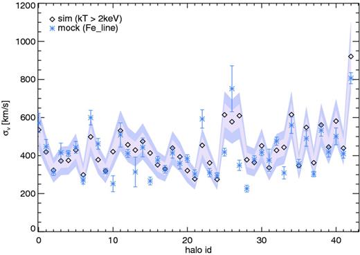
Comparison between the theoretical expectation of the velocity dispersion σv, calculated directly from the simulation (black diamonds and shaded areas) and the value obtained from the spectral fitting of the synthetic XMS spectra obtained with PHOX (blue asterisks with error bars). The id numbers of the 43 haloes in the sample (x-axis) are ordered according to the increasing halo mass, M500.
The expected velocity dispersion of the gas particles residing in the region corresponding to the ATHENA FoV is calculated according to equation (1), weighted by the EM, while the values derived from the X-ray spectra are obtained as described in Section 3.3.1, with error bars corresponding to the 1σ errors to the best-fitting values. As shown in the figure, we find a very good agreement between simulation (intrinsic, ‘true’ solution) and synthetic spectral data (observational detections), namely for ∼74 per cent of the haloes the spectral analysis of the iron lines provides a measure of the gas velocity dispersion, along the l.o.s., within 20 per cent from the expected value (purple, shaded area). We find, in particular, that ∼50 per cent of the haloes show agreement at a level better than ∼10 per cent (internal, pink shaded area in Fig. 5). We remark here that the reference number, or halo id in the figure, is associated with the haloes of the sample in an increasing order for increasing M500.
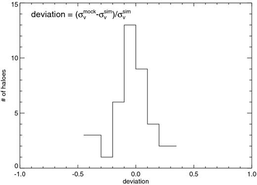
Deviation of the best-fitting σv from the expected value for all the 43 haloes in the sample.
However, we also find outliers in the sample that show deviations up to ∼43 per cent.
4.2.1 Extreme cases in the sample
Given the distribution of the deviations (Fig. 6), we focus on to two subsets of haloes in the sample for which the deviation between simulation and mock data is very minor and most prominent, respectively.
In Fig. 7, we show the l.o.s. velocity structure as calculated from the simulation directly, for both subsets. In particular, the five haloes for which mock and simulated data most disagree are shown in the first and second columns, while the least deviating haloes are presented on the right-hand side of the figure (third and fourth columns). The rows in the figure correspond to a decreasing level of deviation, or agreement, from top to bottom.
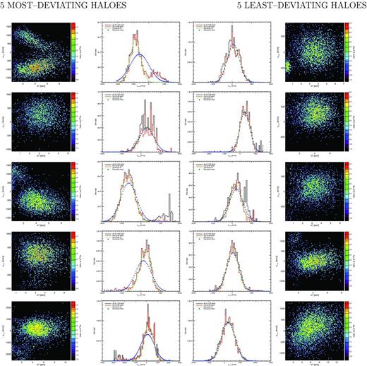
Comparison among the five most deviating (left) and least deviating (right) haloes, according to Fig. 6, for the central region corresponding to the |$2.4\times 2.4\,\text{arcmin}^2$| FoV. The level of deviation, or agreement, decreases from top to bottom. From left to right, the columns refer to (1) vl.o.s.–kT distribution for the gas residing within the selected FoV, colour-coded by EM, for the most deviating haloes, (2) distribution of EM as a function of gas l.o.s. velocity, for the five most deviating haloes, (3) same as (2) and (4) same as (1), but considering the least deviating haloes. In the histograms shown in columns (2) and (3), the curves refer to all the gas particles (black), hot-phase gas (kT > 2 keV; red), Gaussian best fit to the hot-gas distribution (green) and theoretical Gaussian distribution reconstructed from the estimated dispersion of the hot-gas distribution (blue asterisks).
Histograms in the central columns of the figure report the EM distribution as a function of the l.o.s. velocity, for the gas particles in the ATHENA FoV. Black curves refer to all the gas in the region, while the overplotted red histograms only account for the hot-phase gas, i.e. particles for which kT > 2 keV. The reason for selecting the hot gas is that it mostly contributes to the iron line emission, from which the velocity broadening is measured.
It is clear that in the most deviating cases there are substantial substructures within the gas velocity field. The red histograms for the haloes that show best agreement (right-hand column), instead, reflect more regular distributions of the EM as a function of the vl.o.s., indicating more regular velocity fields.
Observationally, the value estimated from the broadening of the spectral lines is assumed to be the dispersion of the Gaussian distribution that best fits the line shape. Therefore, a more detailed comparison should involve the dispersion of the Gaussian function matching the (red) distribution shown, instead of the theoretical value calculated as in equation (1). The green curves in Fig. 7 define the Gaussian fits to the red distributions, whose σgaussv is more directly comparable to the mock spectral results.
As an additional comparison, we also overplot the Gaussian curve (blue asterisks) constructed from the theoretical estimation of the EM-weighted values for gas velocity dispersion (equation 1) and mean l.o.s. velocity. In the most deviating clusters, the evident differences among the green and blue Gaussian curves effectively reflect the deviations discussed above (see e.g. the halo with the largest deviation, top row, left-hand panels in Fig. 7). In particular, the green best-fitting Gaussian clearly fails to capture all the features of the multicomponent velocity distribution, as it most likely happens during the spectral fit. The low level of deviation found for the ‘best’ halo set (right-hand columns) is indeed shown by the good match between best-fitting (green curve) and theoretical (blue asterisks) Gaussian overplotted to the EM–vl.o.s. distributions.
A visualization of the thermodynamical structure of these clusters is also shown in the first and fourth columns of Fig. 7, for the subsets of most deviating and best haloes, respectively. The maps show the vl.o.s.–kT distribution for the gas residing within the selected FoV, colour-coded by EM.
Especially for the most deviating haloes, the substructures in the velocity field unveiled by the histograms are clearly visible, combined with the gas thermal structure.
Despite the deviations discussed, a good overall agreement is found between the intrinsic amplitude of the gas velocity dispersion and the velocity broadening measured directly from mock spectra. This confirms the promising potential of such well-resolved observations, which would most likely allow us to derive reliable and precise constraints on the ICM velocity field.
Moreover, given that the simulation analysis suggests the gas velocity structure in the innermost region (e.g. that covered by the FoV of ATHENA) to be closely traced by that within R500 (see Section 4.1), we will use the latter for our further investigation. Eventually, limitations due to small FoVs could be observationally overcome by multiple pointings covering a larger region.
4.3 LX–T scaling relation
Here, we investigate the impact of the ICM velocity structure on X-ray global properties by focusing on the LX–T relation. The main motivation behind this choice is that, on one hand, the luminosity LX is very well measured in X-ray surveys (e.g. with Chandra, XMM–Newton or the upcoming eROSITA) and, on the other hand, the temperature T provides a good mass proxy, since it is tightly related to the total gravitating mass, which is the most fundamental quantity to characterize a cluster.
LX, also denoted as ‘bolometric X-ray luminosity’, is usually the X-ray luminosity extrapolated to the whole X-ray band, 0.1–100 keV, instead of being calculated in a narrow energy band. None the less, in our case, the computation of the luminosity is limited to the largest energy band defined by the ACIS-I3 response matrix (i.e. 0.26–12 keV), since the difference introduced with respect to the expected bolometric X-ray luminosity is found to be minor.
In Fig. 8, we show the LX–T relation calculated for the simulated haloes (asterisks), from the Chandra synthetic observations of the R500 regions through the l.o.s., obtained with PHOX. As a comparison, we also show the data presented in Pratt et al. (2009, also P09 hereafter) for a sample of 31 nearby galaxy clusters (black diamonds), selected only in X-ray luminosity from the Representative XMM–Newton Cluster Structure Survey (REXCESS).
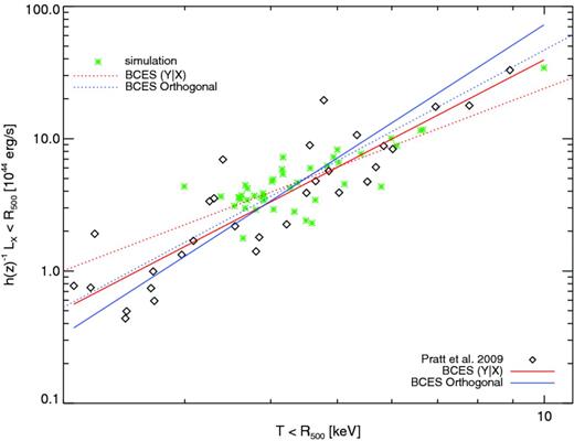
LX–T scaling relation from Chandra mock spectra (green asterisks), for the region of the clusters encompassing R500. Overplotted are the results from P09 (black diamonds). Best-fitting relations are also overplotted (solid lines for P09; dotted lines for simulated haloes of the present work) and correspond to the two linear regression fitting methods adopted: BCES (L∣T) (red) and BCES orthogonal (blue).
4.3.1 Fitting procedure
As done in Pratt et al. (2009), as well as in several similar works (e.g. Reiprich & Böhringer 2002; Arnaud, Pointecouteau & Pratt 2005; Mittal et al. 2011), we adopted the bivariate correlated errors and intrinsic scatter (BCES) regression method by Akritas & Bershady (1996), which accounts for the errors in both LX and T, as well as the intrinsic scatter in the data. The BCES algorithm allowed us to calculate the best-fitting values of slope (α) and normalization (C) for four different regression methods, amongst which we restrict our attention to the BCES (L∣T) and the BCES orthogonal methods. Our primary goal is to find the best fit which minimizes the residuals of both variables at the same time, orthogonally to the linear relation. This is given by the BCES orthogonal method. Additionally, we also explore the results given by the BCES (L∣T) fitting method (analogously to Pratt et al. 2009), which minimizes the residuals in LX. Reasons for this rely on the fact that LX can be treated as the dependent variable, while the temperature can be assumed to be the ‘independent’ one, as closely related to the cluster mass, which is the intrinsic quantity characterizing the system.
Best-fitting relations are overplotted in Fig. 8 for both observational data [solid red and blue lines, for the BCES (L∣T) and the BCES orthogonal method, respectively, from Pratt et al. (2009)] and Chandra synthetic observations of the simulated sample (dotted lines). The linear relations found for the simulated clusters are overall shallower than the observed ones, and, among the two fitting methods considered, the BCES (L∣T) method still provides a shallower slope than the BCES orthogonal case.
In particular, we find a slope α(L∣T) = 1.97 ± 0.23 for the BCES (L∣T) fit and αortho = 2.78 ± 0.3 for the BCES orthogonal fit. As for the normalization of the best-fitting relations, we find C(L∣T) = 6.81 ± 0.39 (1044 erg s−1) and Cortho = 6.11 ± 0.34 (1044 erg s−1), respectively.
We note, however, that our cluster sample probes a smaller dynamical range with respect to observations and, in particular, lacks low-temperature haloes, whose presence might contribute, providing tighter constraints on the slope of the relation.
5 DISCUSSION
5.1 LX–T relation: effects of the velocity structure
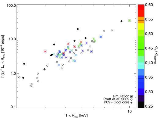
LX–T scaling relation from Chandra mock spectra, for the region of the clusters encompassing R500. Colour code: value of μ = σv( < R500)/σthermal, calculated from gas velocities in the region encompassed by R500. Observational data points (black diamonds) are from P09, with CC clusters marked with thicker black diamonds.
The velocity dispersion σv corresponds to the EM-weighted value calculated directly from the gas particles in the simulation (see Section 4.1). The thermal velocity dispersion, σthermal, is the expected three-dimensional value for the ICM temperature T, reported in the x-axis of the relation. To this purpose of normalizing the non-thermal velocity dispersion to a value characteristic for the halo potential well, the choice of the three-dimensional thermal velocity is equivalent to the one-dimensional value, apart from the constant scale factor |$\sqrt{3}$|. Small values of μ indicate a low level of non-thermal velocity with respect to the characteristic thermal velocity dispersion of the gas.8 For the extreme case of μ ∼ 1, the non-thermal velocity dispersion would equal the thermal value.
The distribution of μ for the 43 simulated clusters is shown in Fig. 10. A significant number of haloes (∼35 per cent) are characterized by a gas velocity dispersion which is larger than 0.4σthermal.
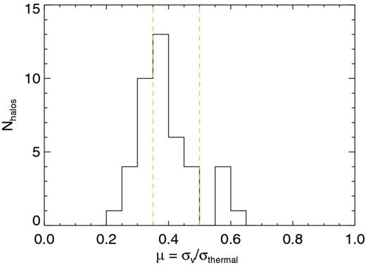
Distribution of μ = σv( < R500)/σthermal, for the sample of 43 simulated clusters. Green, dashed lines correspond to the values μmax = 0.5 and 0.35 used to identify the two subsamples.
In particular, by examining the distribution of μ within the sample, we decide to extract two additional subsamples from the 43 haloes, selected to have a maximum of μmax = 0.5 and 0.35, respectively. The first subsample is intended to exclude the most prominent outliers in the μ distribution, for which the velocity dispersion σv exceeds 50 per cent of σthermal. The smaller subsample contains the haloes with the smallest fraction of μ, indicating that their expected thermal velocity is dominant with respect to σv.
In order to quantify the effects of l.o.s. velocity structure on the resulting scaling relation, we investigated the dependences of best-fitting slope, normalization and scatter on the value of μ, by fitting the LX–T relation for the original sample and for the two subsamples, separately. Results are shown in Fig. 11, where we report both the BCES (L∣T) (red squares) and the BCES orthogonal (blue squares) values.
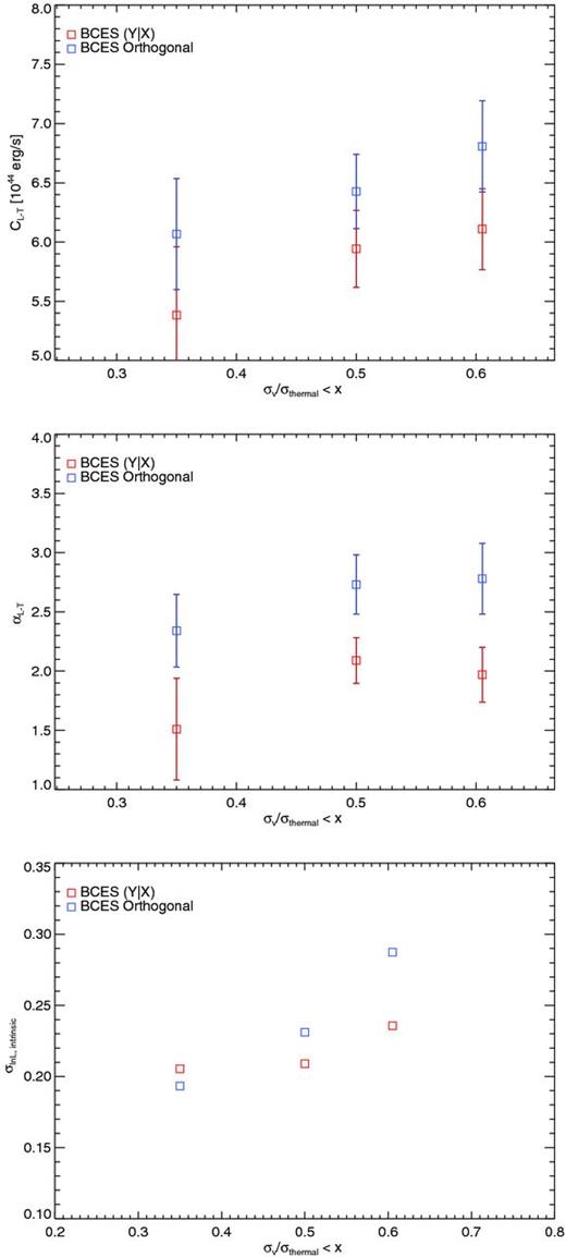
Dependence of normalization (C, top), slope (α, middle) and intrinsic scatter (σlnL, intrinsic, bottom) of the LX–T relation on the maximum μ used to select the corresponding subsample of clusters.
For all the quantities studied, the best-fitting values generally increase with the increasing amplitude of velocity dispersion, relative to the characteristic thermal value. This has significant implications for the intrinsic scatter (calculated here for the luminosity, σlnL, intrinsic9). In fact, the trend found reflects how the scatter in luminosity of the LX–T scaling relation is sensitive to the baryonic physics and can be closely related to complex or disturbed configurations of the ICM velocity field, which are quantified by large values of μ. Essentially, we find that the introduction of clusters with significant non-thermal velocity dispersion, with respect to their typical thermal velocity, augments the scatter in the sample about the best-fitting LX–T relation.
We note from the relation shown in Fig. 9 that the additional characterization of the cluster through the l.o.s. non-thermal velocity dispersion defines a different picture with respect to observations. The observed behaviour of cool-core (CC) and disturbed galaxy clusters shows in fact a distinct separation of the two populations in the LX–T relation (see data points reported in the figure from Pratt et al. 2009), where CC clusters are generally found to occupy the upper envelope of the best-fitting relation (black, thick diamonds in Fig. 9), while morphologically disturbed clusters mostly reside in the lower one. In Fig. 9, however, we find that haloes with the most significant degree of non-thermal motions populate mostly the region above the best-fitting curve. According to this velocity diagnostics, these haloes might be classified as disturbed. We interpret this apparent inconsistency with observations as a different probe for deviation from the regularity of the haloes. Indeed, a deeper analysis of the simulated sample indicates that all the clusters have central electron densities which are sufficiently low to be identified as non-CC clusters, which remove the discrepancy with observed clusters entirely, as further discussed in Section 5.3. Namely, within the population represented by our sample, the quantification of non-thermal velocity dispersion of the gas along the l.o.s. constitutes an additional, complementary method to further discriminate the halo dynamical state.
5.2 Velocity diagnostics: prominent outliers
The velocity diagnostics performed and the distribution of the μ value clearly single out some haloes in the high-velocity tail. This subsample of five clusters includes the most prominent outliers in the LX–T relation, and the exclusion of these haloes turns out to reduce the scatter in the best-fitting relation. Therefore, we further discuss here their thermodynamical structure from the simulation directly, in order to provide an interpretation of the high gas velocities found.
In Fig. 12, we show the spatial distribution of temperature (kT), l.o.s. component of the gas velocity (vl.o.s.) and EM of the five outliers, as well as the vl.o.s.–kT phase diagram, colour-coded by EM. The region of the clusters considered is always that enclosed within the projected R500, along the l.o.s. through the simulation box.
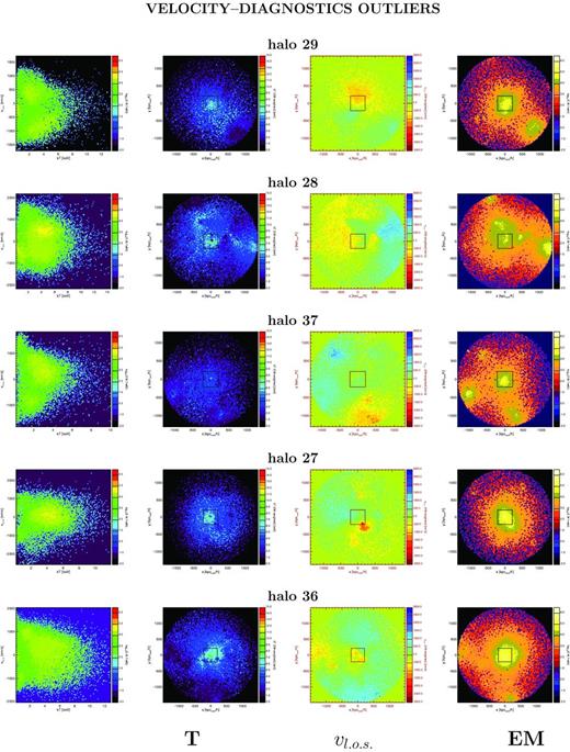
Maps of the ICM thermodynamical status for the five most significant outliers singled out by the velocity diagnostics. Columns, from left to right: (1) vl.o.s.–kT map, colour-coded by EM (considering gas particles within R500); (2) EM-weighted temperature map, projected along the l.o.s.; (3) EM-weighted l.o.s. velocity map projected on to the xy plan (i.e. along the l.o.s.); (4) EM map projected along the l.o.s. Spatial maps in columns (2)–(4) refer to the whole R500 region and overplotted is the ATHENA-like FoV for comparison. From top to bottom, the haloes are ordered such that the value of μ = σv( < R500)/σthermal (equation 6) is decreasing.
Despite the fact that all of these clusters show significant non-thermal motions compared to the characteristic thermal velocity expected, they show different evolutionary states of such velocity patterns.
Clearly, the maps show very different internal structures and the presence among these velocity outliers of both substructured haloes and more regular roundly shaped ones, such as halo 36 especially. The latter, in particular, shows very regular features, no significant substructures and relatively low cooling time (as will be shown in Section 5.3), suggesting that the non-thermal velocities measured are not due to merging or infalling subhaloes but rather characterize intrinsically the ICM. Similar is the case of halo 27, which shows a very regular morphology and structure from all the maps in Fig. 12 and is characterized, however, by both large cooling times and significant non-thermal velocities.
Such examples indeed represent the problematic case where no self-bound substructures are visible in the emission maps, being probably dissolved but not yet fully thermalized, which causes high-velocity streams to persist in the ICM. Here the usual classification of the halo as a regular, not disturbed, cluster and the assumption of thermal motions to dominate the gas pressure support might be misleading.
None the less, we also find more trivial cases, such as haloes 37 and 28, that show significant substructures in the emission maps, reflected in their velocity and temperature structure. This suggests a non-relaxed dynamical configuration, where the subhaloes are still in the form of self-bound objects with an own DM potential and are most likely responsible for driving high-velocity motions. In fact, these clusters deviate significantly from the best-fitting LX–T relation, meaning that the kinetic energy of the infalling substructures has not yet thermalized and the boost in luminosity is not yet followed by the increase of temperature. Similarly, the high velocity measured for halo 29 might be related to a disturbed state of the cluster, for which a subhalo is clearly present from the emission map.
In an observational case of this kind, though, clearly disturbed haloes can be identified and prominent substructures can be explicitly excluded from the analysis.
5.3 Cool-core clusters in the simulated sample
In Fig. 13, we plot the central cooling time, normalized to Hubble time, as a function of central electron density, ne, 0, for all the cluster in the sample. As in Pratt et al. (2009), we define the central values as those calculated at 0.03R500.10 The data reported have been derived from the three-dimensional profiles of the haloes, calculated directly from the simulation.
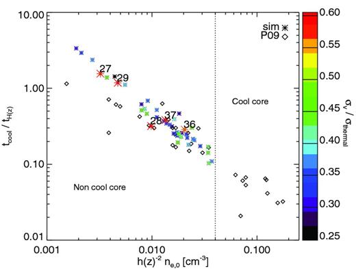
Cooling time versus central electron density, with colour code as in Fig. 9. Asterisks refer to simulated data, while black diamonds represent the observational sample investigated in P09. The dotted line marks the threshold adopted by P09 to define CC systems, i.e. h(z)−2 ne, 0 > 4 × 10⁻² cm−3.
Opposite to the overcooling problem of standard numerical simulations, we show with this figure that no real CCs are present in our sample, as a consequence of the inclusion in the simulations of AGN feedback. In fact, this has the effect of preventing the gas in the hot phase to remain in the central region long enough time to cool and form stars. Comparing to observational data, we do not find haloes populating the region of very short cooling times and high central electron density.
Here, we adopt the same colour code as in Fig. 9 in order to identify the most prominent velocity outliers previously discussed. We note that the five outliers singled out by the velocity diagnostics (Section 5.2) comprise both haloes with very long cooling times and haloes for which the cooling time is only some tenths of the Hubble time. For the latter, although not classified as strong CCs, cooling might be nevertheless important in the central region. With respect to our analysis, this can also be the case of substructured haloes, whenever the approaching subhaloes have not merged yet, namely the first passage through the cluster central region is yet to occur. In such circumstances, the cooling time calculated for the cluster core can also be relatively small, since the innermost region is yet to be affected by the interaction, while the luminosity and velocity fields already are.
Among these haloes with relatively short cooling time, we find two haloes (37 and 28) out of the five clusters with significant non-thermal motions, which reside in the region above the best-fitting LX–T relation. This suggests that there is no real tension between their position in the LX–T plane and the observational evidence of CC clusters occupying that region of the relation. The velocity diagnostics proposed can actually probe different aspects of the cluster state in addition to the usual distinction between CCs and morphologically disturbed clusters.
6 CONCLUSIONS
In this paper, we have presented the study of the ICM velocity structure and its impact on the LX–T scaling relation and cluster status, from hydrodynamical simulations and synthetic X-ray observations of a set of galaxy clusters. Numerical simulations have been performed by means of the treePM/SPH parallel code p-gadget3, including a number of physical processes describing the baryonic component with a level of detail never reached so far, namely cooling, star formation and SN-driven winds (Springel & Hernquist 2003), chemical enrichment from stellar population, AGB stars and SNe (Tornatore et al. 2004, 2007), low-viscosity SPH (Dolag et al. 2005), black hole growth and feedback from AGN. The set of 43 simulated cluster-like haloes has been selected from a medium-resolution cosmological box by requiring M500 > 3 × 10¹⁴ h−1 M⊙. The mock X-ray observations have been obtained with the virtual photon simulator PHOX (Biffi et al. 2012) for both Chandra ACIS-I3 and the XMS originally designed for ATHENA, and used here as prototype for any next-generation X-ray spectrometer capable of reaching very high energy resolution.
From the direct analysis of the gas component in the central part of the simulated haloes, in the projection plane perpendicular to the chosen l.o.s., we find tight relations among different definitions and selection criteria used to calculate the l.o.s. component of the gas velocity dispersion. In order to consistently compare and use results from simulations and mock observations, we always refer to cylinder-like regions which extend throughout the z coordinate of the simulated box, i.e. along the l.o.s. direction. In particular, we find that mass- and EM-weighted velocity dispersions calculated for the gas particles with R500 both correlate closely to the halo M500 and, therefore, can be equivalently employed. Between the two definitions, we concentrate on the EM-weighted velocity dispersion since it is more sensitively related to the gas X-ray emission.
We also find that σ500,EM probes fairly well the velocity dispersion in inner, smaller regions of the clusters, such as the region covered by a small FoV like that of ATHENA. As a fair approximation, we can safely assume the results to be representative of the whole region out to R500, even though single-pointing observations with a telescope of similar FoV of clusters at the considered redshift would only cover their innermost part. On the other hand, small-scale spatial features of the ICM velocity field could be possibly unveiled by the detailed comparison between the large-scale amplitude of the l.o.s. velocity dispersion and the value detectable with ATHENA-like observations.
By applying our virtual telescope, PHOX, to the simulated haloes, the l.o.s. velocity dispersion is derived from the velocity broadening of the Kα iron complex around 6.7 keV in the synthetic X-ray spectra, provided the high energy resolution expected to be reached by such a spectrometer.
Moreover, predictions on σv provided by the simulation and detections mimicked with PHOX show a level of deviation of less than 20 per cent, for 74 per cent of the clusters in the sample. The largest deviations of observed velocities from expected values are significantly dependent on the complicated distribution of the gas velocities and thermal structure (see Fig. 7). In principle, a more detailed modelling of the shape of the spectral emission lines, such as the iron complex used here, rather than the standard Gaussian fit, should permit us to derive more accurate measures of the l.o.s. velocity dispersion of the gas, accounting for multiple (thermal) components in the velocity field.
Given the ideal case of a similar X-ray spectrometer at high resolution, we base our further investigation on the simulation results. Indeed, this is further suggested by the good agreement between mock data and simulation and therefore we utilize the σ500,EM obtained directly from the simulation to constrain the impact of velocity structure on to X-ray observables, such as luminosity and temperature.
In principle, as soon as high-precision X-ray spectroscopy will become available for real observations, we will be able to safely employ the detected values of the ICM non-thermal velocity dispersion for studies of real galaxy clusters as well. Possibly, this will be already explored, for instance, in the case of the brightest clusters by means of the upcoming ASTRO-H satellite, due to be launched in 2014, for which a energy resolution of 7 eV at 0.3–12 keV is expected.
From the synthetic Chandra spectra obtained with PHOX, we were able to estimate observed bolometric luminosity, extrapolated to the entire X-ray band, and temperature, for the ICM residing within R500 in the projection plane. The LX–T scaling relation constructed from these mock data generally agrees with real observations, e.g. from Pratt et al. (2009). By using the BCES linear regression fitting method (Akritas & Bershady 1996), we assume a linear relation between LX and T in the log–log space and determine the best-fitting slope and normalization of the LX–T for our 43 simulated clusters, finding a shallower slope with respect to the results reported in Pratt et al. (2009). In the fitting procedure, we explore both the BCES (L∣T) and BCES orthogonal methods, where the former treats the luminosity as dependent variable and minimizes its residuals, while the latter implies both variables, L and T, as independent variables and minimizes the orthogonal distances to the linear relation.
As a step forward, we include the information obtained about the ICM velocity dispersion along the l.o.s. in order to investigate the effects on slope, normalization and intrinsic scatter of the best-fitting LX–T relation.
Interestingly, the exclusion from the original sample of the haloes with largest velocity dispersion (normalized to the characteristic thermal value associated with their temperature) has the effect of reducing the scatter in the LX–T relation, as shown by the trend in Fig. 11 (bottom panel). The increasing trend of slope and scatter, in particular, evokes a dependence on the contamination of the sample by haloes which show significant fraction of non-thermal velocity, although the results would need a larger statistics to be more strongly confirmed, especially at the low-temperature end of the relation, which is not probed by our sample.
Nevertheless, an interesting indication of our velocity diagnostics is that even haloes with fairly regular appearance or relatively low central cooling time can be characterized by high non-thermal velocities of the gas along the l.o.s., deviating therefore from the expected scaling relations among global properties (e.g. the LX–T scaling law). Additional information on the velocity structure of the clusters might therefore be helpful to constrain their state better. Observationally, for the clusters where the velocity measurements are indeed achievable, this can be used as complementary characterization to the usual morphological or cooling-time-based approach.
As a promising future perspective, we expect high-precision X-ray spectroscopy to provide valuable information on the non-thermal velocity structure of the ICM in galaxy clusters along the l.o.s., which can be safely assumed to trace the intrinsic gas motions of the cluster despite the effects due to projection and instrumental response. This will be certainly fundamental to correctly determine the total mass in clusters and characterize in more detail the deviation of real clusters from the hydrostatic equilibrium at the base of X-ray mass estimates as well as the divergence from the self-similarity of the haloes expected from theoretical models.
KD acknowledges the support by the DFG Priority Programme 1177 and additional support by the DFG Cluster of Excellence ‘Origin and Structure of the Universe’. The underlying cosmological simulations were performed within the DEISA/DECI-6 initiative under the project ‘MagPath’.
Note that R500 is defined here as the radius enclosing the region of the cluster whose mean density is 500 times the mean density of the Universe. This encompasses therefore a larger region with respect to the usual definition of R500, where the overdensity is instead defined with respect to the critical density of the Universe.
In the case of haloes fitted with a two-component model, we assume here the hotter temperature to be representative of the dominant gas component
We recall here that EM = ∫nenH dV.
In the log space, errors are transformed as Δ logx = loge × (Δx)/(2x), where Δx is the difference between the upper and lower boundary of the error range around the quantity.
In fact, the thermal component of the velocity is not included within σv, which traces macroscopic motions of the gas elements in the simulation. Analogously, the value measured from the velocity broadening of spectral lines, used for comparison in Section 4.2, does not include the thermal component either.
We report the final value by considering the natural logarithm, ln, for comparisons to Pratt et al. (2009), although the equations and the logarithm space mentioned in the paper usually refer to log = log10.
While for global properties as LX or T the difference in the definition of R500 is not crucial, here we also calculate the Δ = 500 overdensity with respect to the critical density of the Universe, in order to compare as consistently as possible against the observational data. In fact, the definition is particularly relevant in order to evaluate the values of cooling time and density at exactly the same radius, being not mean values within a region but rather local values.
REFERENCES
APPENDIX A: TREATMENT OF CHEMICAL ABUNDANCES IN PHOX
Dealing with galaxy clusters, the main emission components in the X-ray regime are constituted by bremsstrahlung continuum and emission lines from heavy elements.
Usually, simulations of the X-ray emission from hydrodynamically simulated clusters assume the average value of one-third the solar metallicity, consistent with the average metallicity measured for real clusters. With respect to previous hydrosimulations, however, the run analysed here provides full information on the chemical enrichment of the gas, tracing its composition with 10 elements, namely He, C, Ca, O, N, Ne, Mg, S, Si and Fe. An additional field for each gas particle accounts also for the total mass in all the remaining metals.
Therefore, the available abundances of the individual elements, He included, are read and used to calculate the contribution of each element to the final spectrum.
APPENDIX B: THE SIMULATED SAMPLE
In order to have a visual presentation of the sample discussed in this work, we show in Fig. B1 the EM for the 43 clusters, for the cylinder-like region along the l.o.s., encompassed by R500 around each cluster.
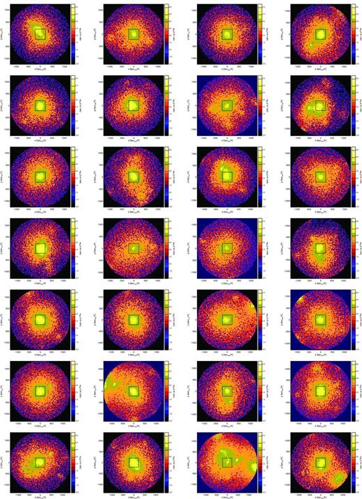
Visualization of the 43 most massive galaxy clusters in the simulated sample. The panels show the EM maps in the plane perpendicular to the l.o.s., within the R500 region of each cluster.
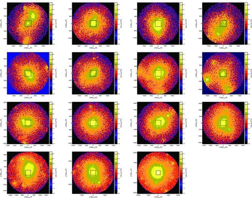
– continued
