The clustering of galaxies in the SDSS-III Baryon Oscillation Spectroscopic Survey: a large sample of mock galaxy catalogues

Manera, Marc; Scoccimarro, Roman; Percival, Will J.; Samushia, Lado; McBride, Cameron K.; Ross, Ashley J.; Sheth, Ravi K.; White, Martin; Reid, Beth A.; Sánchez, Ariel G.; de Putter, Roland; Xu, Xiaoying; Berlind, Andreas A.; Brinkmann, Jonathan; Maraston, Claudia; Nichol, Bob; Montesano, Francesco; Padmanabhan, Nikhil; Skibba, Ramin A.; Tojeiro, Rita; Weaver, Benjamin A.

doi:10.1093/mnras/sts084

Abstract

We present a fast method for producing mock galaxy catalogues that can be used to compute the covariance of large-scale clustering measurements and test analysis techniques. Our method populates a second-order Lagrangian perturbation theory (2LPT) matter field, where we calibrate masses of dark matter haloes by detailed comparisons with N-body simulations. We demonstrate that the clustering of haloes is recovered at ∼10 per cent accuracy. We populate haloes with mock galaxies using a halo occupation distribution (HOD) prescription, which has been calibrated to reproduce the clustering measurements on scales between 30 and 80 h⁻¹ Mpc. We compare the sample covariance matrix from our mocks with analytic estimates, and discuss differences. We have used this method to make catalogues corresponding to Data Release 9 of the Baryon Oscillation Spectroscopic Survey (BOSS), producing 600 mock catalogues of the ‘CMASS’ galaxy sample. These mocks have enabled detailed tests of methods and errors, and have formed an integral part of companion analyses of these galaxy data.

galaxies: haloes, large-scale structure of Universe

1 INTRODUCTION

Galaxy surveys such as the Baryon Oscillation Spectroscopic Survey (BOSS; Schlegel, White & Eisenstein 2009a; Eisenstein et al. 2011), WiggleZ (Drinkwater et al. 2010), the Hobby-Eberly Telescope Dark Energy Experiment (HETDEX, Hill et al. 2004) and the Dark Energy Survey¹, designed to cover large areas of the sky, are currently leading the effort to measure cosmological parameters using the observed clustering of galaxies and quasars. In future, the baton will be passed to projects such as eBOSS, BigBOSS (Schlegel et al. 2009b), Euclid (Laurejis et al. 2011) and the Large Synoptic Survey Telescope (LSST, Abell et al. 2009). These projects will cover large volumes of the Universe, and observe millions of galaxies in order to make precise measurements. BOSS aims to determine the cosmic expansion rate H(z) with a precision of 1 per cent at redshifts z ≃ 0.3 and 0.6, and with 1.5 per cent at z ≈ 2.5, by means of accurately measuring the scale of the baryon acoustic peak (Eisenstein et al. 2011). The first steps towards this goal are presented in a companion paper (Anderson et al. 2012), which provides the highest precision measurement of the baryon acoustic scale to date.

Such large-scale clustering measurements require an estimate of their joint variances in order to produce reliable cosmological constraints. This is usually calculated in matrix form, and one could get this matrix by running a large number of N-body simulations and generating galaxy mocks. However, this would be computationally very expensive and, as surveys probe increasingly larger scales, impractical. If only a small number of realizations are used, then the estimated covariance matrix can be very noisy. There have been several suggestions in the literature on how to deal with this problem.

When analysing the second Sloan Digital Sky Survey (SDSS)-II Data Release 7 (DR7) luminous red galaxies, Xu et al. (2012) used a smooth approximation to the mock covariance matrix. This technique involves fitting an analytic form to a covariance matrix computed from a relatively small number of N-body galaxy mock catalogues, using a maximum likelihood approach with a number of underlying assumptions. This smoothing technique is critical in the regime of a small number of mocks, but would be obsolete if a sufficiently large number of mocks were available, requiring fewer underlying assumptions in the estimation of the covariance matrix.

Alternatively, the lognormal model has been used to generate large numbers of mock catalogues, from which covariance matrices are calculated (Cole et al. 2005; Percival et al. 2010; Blake et al. 2011). Because of its simplicity this approach is fast. However, it does not properly account for non-Gaussianities and non-localities induced by non-linear gravitational evolution.

Another method of estimating covariances is jackknife resampling, which allows errors to be estimated internally, directly from the data (Krewski & Rao 1981; Shao & Tu 1995). It does however require some arbitrary choices (such as the number of jackknife regions, for example) and its performance is far from perfect (see e.g. Norberg et al. 2009). It also will not include fluctuations on the scale of the survey.

Analytic efforts to estimate covariance matrices directly from theory, which go beyond a simple rescaling of the linear Gaussian covariance, must deal with non-linear evolution, shot-noise, redshift-space distortions (RSD), and the complex mapping between galaxies and matter (Hamilton, Rimes & Scoccimarro 2006; Sefusatti et al. 2006; Pope & Szapudi 2008; de Putter et al. 2012; Sefusatti et al., in preparation). Thus, they tend to be complicated and difficult to make accurate. Such techniques though may be able to help translate matrices between cosmological models.

In this paper, we present a new method for generating galaxy mocks that is significantly faster than basing samples on N-body simulation results. This follows the main ideas put forwards in the PTHalos method of Scoccimarro & Sheth (2002), but the implementation is overall simpler and differs in some key aspects; the most relevant being that we do not use a merger tree to assign haloes within big cells of the density field but instead we obtain the haloes more precisely using a halo finder. This method is fast because it is based on a matter field generated using second-order Lagrangian perturbation theory (2LPT), but it still allows us to include the most important non-Gaussian corrections relevant for covariance matrices described by the trispectrum.

We use this method to create 600 mock galaxies catalogues occupying the volume that can accommodate the SDSS-III DR9 BOSS CMASS sample. This sample contains 264 283 high-quality spectroscopic galaxy redshifts in the range of 0.43 < z < 0.7 distributed over an angular footprint of 3 275 deg². It has the largest effective volume of any galaxy sample observed to date (see Anderson et al. 2012 for further details). We apply the CMASS DR9 selection function to our mock catalogues, thereby including the full effect of the survey geometry. We thus provide the means by which statistical errors are determined for the CMASS DR9 sample.

Notationwise, in this paper, we keep the name ‘PTHalos’ for our implementation, and, when appropriate, we explicitly distinguish it from the implementation of Scoccimarro & Sheth (2002). The haloes that are obtained by the PTHalos method/code are named PThalos (with lower case H).

This paper has two parts. First, we describe our PTHalos method and compare (and calibrate) our PThalos with haloes from N-body simulations from the LasDamas collaboration (McBride et al., in preparation). In the second part, we populate the PThalos with mock galaxies in a way that matches the CMASS sample. These mocks have been used in several analyses of BOSS DR9 data, including the study of systematics (Ross et al. 2012), the determination of the baryon acoustic oscillations (BAOs) scale (Anderson et al. 2012), RSD (Reid et al. 2012; Samushia et al. 2012), evolution of galaxy bias (Tojeiro et al. 2012a,b), the concordance with the Λ cold dark matter (ΛCDM) model (Nuza et al. 2012) and the full shape of the correlation function (Sánchez et al. 2012). Note that the use of the mocks is not limited to only providing covariance matrices. For instance, by using mocks one can assess the level of expected chance correlation between galaxies and systematics (e.g. Ross et al. 2012).

Galaxy PTHalos mocks will be made publicly available.² A table with the monopole of the correlation function and the covariance matrix is given at the end of the paper. All log values in this paper are in base 10.

2 OVERVIEW OF THE METHOD

Our goal is to develop a fast method for generating galaxy mocks, such that covariance matrices can be computed accurately for galaxy samples such as the CMASS DR9 (Anderson et al. 2012) and the methods of analysis can be tested for bias and relative accuracy. The basic steps in the method can be summarized as follows.

Create a particle-based 2LPT matter field (as described in Section 4).
Identify haloes using a friends-of-friends (FoF; Davis et al. 1985) halo finder with an appropriately chosen linking length. We argue that, for the BOSS mean redshift, this linking length should be ∼0.38 times the comoving interparticle distance; see Section 6. We name the haloes identified in the 2LPT matter field 2LPT haloes.
Assign masses to the 2LPT haloes by imposing a mass function that agrees with N-body simulations. We name the haloes with the new masses PThalos.
Populate the PThalos with galaxies using a halo occupation distribution (HOD) algorithm calibrated to fit the observational data.
Apply the survey angular mask and galaxy redshift distribution.

We validate the first three steps by comparing our method with the clustering of haloes in the N-body simulations whose halo abundances we have matched. We then apply the final steps by calibrating the HOD to the CMASS DR9 data set. Finally, we generate 600 mocks of CMASS galaxies with DR9 geometry and redshift selection.

The gain in runtime achieved by generating PTHalos galaxy mock catalogues compared to creating mock catalogues from N-body simulations comes from the first step: for the particle numbers used here, 2LPT is about three orders of magnitude faster than N-body simulations. The time taken to make mock catalogues in PTHalos is dominated by the subsequent steps, and thus the speedup factor at the end of the procedure is reduced to about two orders of magnitude.

3 OVERVIEW OF THE BOSS CMASS DR9 GALAXIES

BOSS, part of the SDSS-III (Eisenstein et al. 2011), is an ongoing survey measuring spectroscopic redshifts of 1.5 million galaxies, 160 000 quasars and a various ancillary targets. BOSS uses SDSS CCD photometry (Gunn et al. 1998, 2006) from five passbands (u, g, r, i, z; e.g. Fukugita et al. 1996) to select targets for spectroscopic observation.

The BOSS CMASS galaxy sample is selected with colour–magnitude cuts, aiming to produce a roughly volume-limited sample in the redshift range of 0.4 < z < 0.7, and results in a sample that is approximately stellar-mass limited. These galaxies have a bias of ∼2 and most are central galaxies of haloes of 10¹³ M_⊙, with a non-negligible fraction (∼10 per cent) being satellites in more massive haloes (White et al. 2011).

DR9 includes data taken up to the end of 2011 July. The details of the catalogue and mask used for the large-scale structure analyses are explained in Anderson et al. (2012), and an analysis of potential systematic effects is presented in Ross et al. (2012). DR9 covers approximately 3344 deg² of sky (containing 264 283 usable redshift galaxies over 3275 deg²) of which 2635 deg² (containing 207 246 galaxies) are in the Northern Galactic cap (NGC) and 709 deg² (containing 57 037 galaxies) are in the Southern Galactic cap (SGC), as shown in Fig. 1. The NGC and SGC have slightly different redshift distribution of galaxies; we show their normalized redshift distributions, n(z), in Fig. 2. NGC and SGC mock catalogues have been generated according to thesedistributions.

Figure 1.

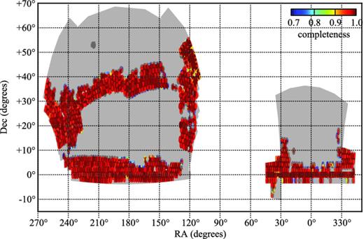
The Northern Galactic cap (NGC) and Southern Galactic cap (SGC) footprint of the CMASS DR9 galaxy sample.

Open in new tab Download slide

Figure 2.

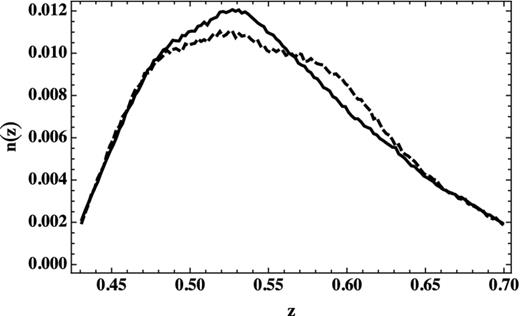
Normalized redshift distribution of galaxies in the NGC (solid) and SGC (dashed) CMASS DR9 sample.

Open in new tab Download slide

4 SUMMARY OF 2LPT

Basics of Lagrangian perturbation theory

The Lagrangian description of structure formation (Buchert 1989; Moutarde et al. 1991; Hivon et al. 1995) relates the current (or Eulerian) position of a mass element, |${\boldsymbol x}$|⁠, to its initial (or Lagrangian) position, |${\boldsymbol q}$|⁠, through a displacement vector field |${\boldsymbol \Psi }({\boldsymbol q})$|⁠,

\begin{equation} {{\boldsymbol x}}= {{\boldsymbol q}}+ {\boldsymbol \Psi }({{\boldsymbol q}}). \end{equation}

(1)

The displacements can be related to overdensities by (Taylor & Hamilton 1996)

\begin{equation} \delta ({\boldsymbol k}) = \int {\rm d}^3 {\boldsymbol q}\ {\rm e}^{-{\rm i} {\boldsymbol k}\cdot q} \left[{\rm e}^{-{\rm i} {\boldsymbol k}\cdot {\boldsymbol \Psi }({\boldsymbol q})} - 1\right]. \end{equation}

(2)

Analogous to Eulerian perturbation theory, LPT expands the displacement in powers of the linear density field, δ_L,

\begin{equation} {\boldsymbol \Psi } = {\boldsymbol \Psi }^{(1)} + {\boldsymbol \Psi }^{(2)} + \cdots \;, \end{equation}

(3)

with |${\boldsymbol \Psi }^{(n)}$| being nth order in δ_L. First order in LPT is equivalent to the well-known Zel’dovich approximation (ZA).

The equation of motion for particle trajectories x(τ) is

\begin{equation} \frac{{\rm d}^2 {{\boldsymbol x}}}{{\rm d} \tau ^2} + {\cal H}(\tau ) \ \frac{{\rm d} {{\boldsymbol x}}}{{\rm d} \tau }= - \nabla \Phi , \end{equation}

(4)

where ∇ is the gradient operator in Eulerian coordinates x and τ is conformal time. Here, Φ denotes the gravitational potential, and |${\cal H}=\frac{{\rm d} {\rm ln} a}{{\rm d}\tau }=Ha$| denotes the conformal expansion rate. H is the Hubble factor and a is the scale factor.

Substituting equation (1) into equation (4) and solving the equation at linear order gives the Zel’dovich (1970) approximation (ZA),

\begin{equation} \nabla _q \cdot {\boldsymbol \Psi }^{(1)}= -D_1(\tau ) \ \delta ({\boldsymbol q}), \end{equation}

(5)

where we have taken a gradient of equation (4) and used the Poisson equation to relate Φ and δ(q). Here, δ(q) denotes the Gaussian density field imposed by the initial conditions and D₁(τ) is the linear growth factor. In equation (5) the gradient is in Lagrangian coordinates q, while in equation (4) it is in Eulerian coordinates; the two are related by the Jacobian of the coordinate transformation.

The solution to second order describes the correction to the ZA displacement due to gravitational tidal effects and reads

\begin{equation} \nabla _q \cdot {\boldsymbol \Psi }^{(2)}= \frac{1}{2} D_2(\tau ) \sum _{i \ne j} \left[\Psi _{i,i}^{(1)} \Psi _{j,j}^{(1)} - \Psi _{i,j}^{(1)} \Psi _{j,i}^{(1)}\right], \end{equation}

(6)

where the comma followed by a coordinate denotes partial derivative in that direction.

Since Lagrangian solutions up to second order are curl-free, it is convenient to define two Lagrangian potentials ϕ⁽¹⁾ and ϕ⁽²⁾ (⁠|${\boldsymbol \Psi ^{(i)}}=\nabla _q\phi ^{(i)}$|⁠), so that the solution up to second order reads

\begin{equation} {\boldsymbol x}({\boldsymbol q}) = {\boldsymbol q}-D_1\ \nabla _q \phi ^{(1)} + D_2\ \nabla _q \phi ^{(2)}. \end{equation}

(7)

Likewise one can solve for the velocity field, which reads

\begin{equation} {\boldsymbol v} = -D_1\ f_1\ H\ \nabla _q \phi ^{(1)} + D_2\ f_2\ H\ \nabla _q \phi ^{(2)}. \end{equation}

(8)

Here, |$v \equiv \frac{{\rm d} {\boldsymbol x}}{{\rm d} t}$| is the peculiar velocity, t denotes cosmic time, |$f_i=\frac{{\rm d}{\rm ln} D_i}{{\rm d}{\rm ln} a}$| and D₂ denotes the second-order growth factor. To better than 0.6 per cent accuracy,

\begin{equation} D_2(\tau ) \approx -\frac{3}{7} D_1^2(\tau ) \Omega _{\rm m}^{-1/143}, \end{equation}

(9)

for values of |$\Omega _\Lambda$| between 0.01 and 1 (Bouchet et al. 1995).

To generate the 2LPT displacement we used an algorithm that takes advantage of fast Fourier transforms (FFT) and is described in detail in Scoccimarro (1998). Although this algorithm assumes Gaussian initial conditions, it can be extended to treat non-Gaussian initial conditions given by any factorizable primordial bispectrum (Scoccimarro et al. 2012), and a parallel version of such code is publicly available.³ In this paper we only consider Gaussian initial conditions, although the same procedure can be applied to the primordial non-Gaussian case.

Compared to Scoccimarro & Sheth (2002) our implementation of 2LPT differs only in the smoothing applied to the linear density field before constructing the Zel’dovich displacement field. To reduce the effects of orbit crossing (where LPT breaks down), they impose a cut-off in the linear spectrum, similar to the standard truncated ZA (Coles, Melott & Shandarin 1993). We do not follow this approach as, rather than using their merger tree method to identify haloes, here we identify haloes by applying the FoF algorithm to the 2LPT field with a modified linking length. The theoretical motivation for the choice of linking length can be derived from the spherical collapse in 2LPT dynamics (see Section 6.1). In order to preserve this theoretical choice, we would like to change the linear density field on smoothing scales of the order of the Lagrangian size of haloes as little as possible, while at the same time not have excessive orbit crossing effects for the haloes that host the galaxies we are interested in. These competing requirements become increasingly difficult to satisfy as the halo mass we are interested in decreases. Although we have not done an exhaustive investigation, a smoothing window described the linear density field Fourier amplitudes multiplied by e^{−k/(4 + k)/2} (with k in h Mpc⁻¹) works reasonably well for the halo mass range relevant for our purposes; see Section 6. On top of this, there is of course a sharp cut-off in the linear spectrum at the Nyquist frequency of the particle grid used to generate the fields (with grid size N_grid = 1280).

LPT has been used to model BAOs (Matsubara 2008a,b; Padmanabhan & White 2009; Padmanabhan, White & Cohn 2009). For a more detailed explanation of 2LPT, see Bernardeau et al. (2002, and references therein).

5 COSMOLOGY AND RESOLUTION SPECIFICATIONS

We have produced halo and galaxy mocks using two different sets of ΛCDM cosmological parameters. The first set has been chosen to match that of the N-body simulations we use to calibrate the PTHalos method, while the second set has been chosen to have values closer to those expected from observations.

LasDamas cosmology.

The fiducial parameters for this cosmology are as follows: Ω_m = 0.25, |$\Omega _\Lambda =0.75$|⁠, Ω_b = 0.04, h = 0.7, σ₈ = 0.8 and n_s = 1. These parameters were used by the LasDamas collaboration⁴ which produced a suite of large N-body cosmological dark matter simulations (McBride et al., in preparation). These simulations were run with a Tree-PM code gadget-ii (Springel 2005) and a FFT grid size of 2400 points in each dimension. Each simulation covers a cubical volume of a box size L = 2400 Mpc h⁻¹, and has 1280³ dark matter particles. We have created PThalos mocks assuming the same cosmology and resolution parameters, so as to compare halo clustering in each of the 40 N-body simulation runs, and thus calibrate our method. As shown in Section 6, we achieve a 10 per cent accuracy in the clustering of haloes.

WMAP cosmology.

The second ΛCDM cosmology that we consider has the following parameters: Ω_m = 0.274, |$\Omega _\Lambda =0.726$|⁠, Ω_b = 0.04, h = 0.7, σ₈ = 0.8 and n_s = 0.95. These are the same as those used to analyse the first semester of BOSS data (White et al. 2011) and from the fiducial model for the Anderson et al. (2012) analysis; they are within 1σ of the best-fitting 7-year Wilkinson Microwave Anisotropy Probe (WMAP7) concordance cosmological model (Larson et al. 2011).

We have two simulations of 3000³ particles and cubical box size of L = 2750 Mpc h⁻¹ with which we compare results. These simulations were performed with the Tree-PM code described in White et al. (2010), which has been compared to a number of other codes and shown to achieve the same precision level for such simulations (Heitmann et al. 2008). We use one of these simulations in Section 6.5.

Resolution parameters.

We run 2LPT for our mocks in a cubic box of size L = 2400 Mpc h⁻¹ with N = 1280³ particles. This matches the specifications of the LasDamas–Oriana simulations, and allows us to easily match the Fourier phases in 2LPT runs to those of the Oriana simulations, thus allowing a direct comparison for each realization. With these parameters the mass resolution for the LasDamas and WMAP cosmologies is M_part = 45.7 × 10¹⁰ and 50.1 × 10¹⁰ M_⊙ h⁻¹, respectively. The cubical box was matched to the CMASS DR9 geometry as explained in Section 8.2.

6 PT HALOS

PThalos are created in two steps. The first step is to generate a 2LPT field, as described in Section 4, which is traced by means of a distribution of particles. Based on this field, halo positions and raw masses are found using a FoF algorithm, which links all pairs of particles separated by a distance d ≤ b. This algorithm has become a standard technique and has been used extensively in astrophysics and cosmology since Davis et al. (1985). Using the LasDamas simulations we calibrated the FoF linking length, and set b = 0.38 times the mean interparticle separation as the value for generating mocks. Note that this linking length is substantially larger than the usual choice, b = 0.2, in N-body simulations. Section 6.1 shows that this choice is motivated by 2LPT dynamics.

The second step of the method is a reassignment of halo masses. Respecting the ordering given by the FoF number of particles, 2LPT halo masses are changed so that the mean mass function of PThalos matches a given fiducial mass function. The underlying understanding here is that the ranking of the masses is more accurate than their exact values, which will vary according to the definition of halo boundaries, both in N-body simulations and 2LPT runs.

Note that, given an input mass function for PThalos, a fixed 2LPT halo mass always corresponds to the same PThalo mass. That is, the mapping of the masses is between the mean of 2LPT realizations of the mass function and the targeted fiducial one. In this way, the scatter of the measured mass function between 2LPT realizations is translated, as expected, into a scatter of the PThalos mass function.

In this paper, the PThalos realizations with the LasDamas cosmology use, as an input, the mass function of the LasDamas N-body simulations. The PThalos realizations with WMAP cosmology use as input the mass function of Tinker et al. (2008), and adopt the definition of dark matter haloes that correspond to overdensities 200 times the mean background density.

6.1 Linking length: theoretical motivation

The appropriate FoF linking length in N-body simulations can be estimated as follows. Given Ω_m and |$\Omega _\Lambda$| one uses a fitting function (see equation 11) to compute the virial overdensity Δ_vir of haloes within the spherical infall model. For the LasDamas cosmology, Δ_vir = 377 relative to the mean background density, at redshift zero.

Then, assuming an isothermal profile for the dark matter halo, one can relate the mean density of the halo to the density at the virial radius, i.e. ρ_Rvir = Δ_vir/3. This density is converted to a mean separation of particles by assuming that the density at the virial radius is equal to that of two particles in a sphere of radius b. For the LasDamas cosmology, this gives b = 0.156 in units of the mean interparticle separation. For an Einstein–de Sitter cosmology, Ω_m = 1 and b = 0.2, which is the value most commonly used in the literature.

Because the 2LPT dynamics does not capture the non-linear dynamics of virialization, it yields halo densities that consistently differ from the N-body densities. Consequently, the FoF linking length of 2LPT matter field, b_2LPT, needs to be rescaled from the value used in N-body simulations, b_sim. The simplest rescaling is given by

\begin{equation} b_{{\rm 2LPT}} = b_{{\rm sim}} \left( \frac{\Delta _{{\rm vir}}^{{\rm sim}}}{\Delta _{{\rm vir}}^{{\rm 2LPT}}} \right)^{1/3} \;. \end{equation}

(10)

Both the halo virial overdensity in N-body simulations, Δ^sim_vir, and its corresponding value in the 2LPT field, Δ^sim_2LPT, are easy to compute. For the N-body case we take the value of Bryan & Norman (1998),

\begin{equation} \Delta _{\rm vir}^{\rm sim}=(18\pi ^2+82(\Omega _{\rm m}(z)-1)-39(\Omega _{\rm m}(z)-1)^2) /\Omega _{\rm m}(z), \end{equation}

(11)

where

\begin{equation} \Omega_m(z)=\Omega_m (1+z)^3 (H(0)/H(z) ), \end{equation}

(12)

which gives Δ_vir = 244 at redshift z = 0.52. We choose this redshift because it is the redshift at which we will compare with LasDamas simulation outputs, and it is close to the mean redshift of the BOSS CMASS sample, for which we want to produce galaxy mock catalogues.

The Lagrangian Δ^2LPT_vir can be easily obtained from the relation between Lagrangian and Eulerian fields, which are related by the determinant (Jacobian) of the transformation of equation (1),

\begin{equation} \delta _{\rm LPT} = \left[ {{\rm Det}}(1+ \mathrm{\partial} \Psi _i/\mathrm{\partial} q_j) \right]^{-1} -1\;. \end{equation}

(13)

Having solved equations (5) and (6), and thus knowing Ψ at second order, this equation can be rewritten in terms of the growth factor. Then, assuming spherical symmetry for simplicity, it reads

\begin{equation} \delta _{\rm 2LPT} = \left[ 1-\frac{\delta _0}{3}\left(D_1-\frac{\delta _0}{3}D_2\right) \right]^{-3} -1\;, \end{equation}

(14)

where δ₀ is the overdensity at the initial time. Since we know from spherical collapse in Eulerian dynamics that a halo has virialized when its linear density fluctuation is D₁δ₀ = 1.686, we can predict the 2LPT overdensity of at this same linear density to be Δ^2LPT_vir = δ_vir^2LPT + 1 = 35.43 relative to the mean background density.

Therefore, using equation (10), we find that to conduct a robust comparison between PThalos and N-body haloes of linking length of b = 0.2, we need to use a linking length of b = 0.38 in the 2LPT field. It is worth emphasizing that this predicted value is approximate. A better value can be determined by comparing the clustering of haloes between 2LPT and N-body simulations. This process is described in the next section, where we find that the values around b ∼ 0.37 (including 0.38) work very well at the 10 per cent level.

In principle, one can use spherical overdensity (SO) methods to identify haloes instead of the FoF algorithm (Lacey & Cole 1994). A similar procedure to that discussed in Section 6.1 could then be used to match the SO density parameter in N-body simulations to 2LPT simulations.

6.2 Linking length: calibration with N-body simulations

In order to test the linking length that we need to use to find PThalos, we have run a 2LPT simulation at z = 0.52 with the same Fourier phases and amplitudes as that of one of the Oriana simulations from the LasDamas collaboration.

We obtained haloes from the 2LPT dark matter field using different linking lengths close to the value given by equation (10). The 2LPT haloes do not have a correct mass function. These haloes become PThalos once we change the masses to match the mass function of the N-body simulation. We then computed the cross-power spectrum between the PThalos and the N-body matter field, P_{hm, pthalos}(k), and the cross-power spectrum between the N-body haloes and N-body matter field, P_{hm, sim}(k), where these latter haloes, from LasDamas, were obtained with b = 0.2.

The comparison between these two spectra gives a measure of accuracy of the bias of the 2LPT haloes. In particular, we are interested in the ratio P_{hm, pthalos}/P_{hm, sim} since this is equivalent to the ratio of the halo bias factors. Note that we have computed the cross-power spectra and not the autopower spectra since in this case we do not need to correct our estimator for shot noise.

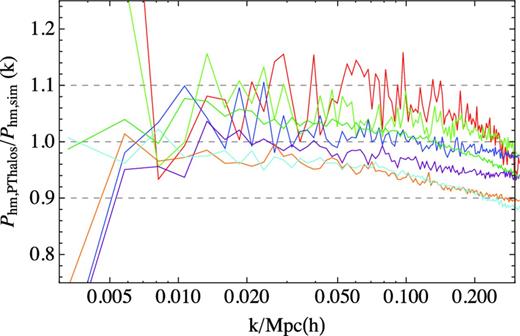
The results are shown in Figs 3–5. Fig. 3 shows the ratio P_{hm, pthalos}/P_{hm, sim} of the million most massive haloes as a function of the wavenumber k for different values of the linking length. We see that, as we increase the linking length, the ratio of the cross-powers decreases. There is a range of linking lengths around b ∼ 0.37 for which the ratio of the bias is within 10 per cent. The predicted value b = 0.38, as computed using equation (10), is well within this range.

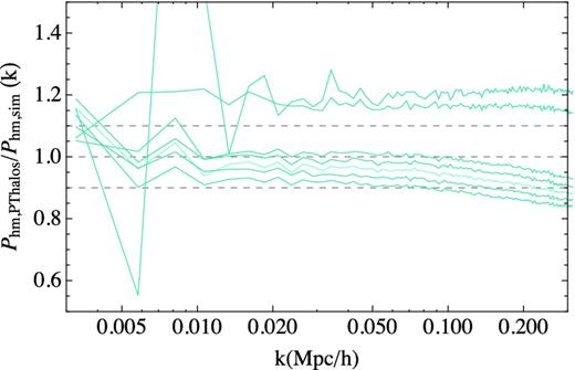
Ratio between PTHalos and N-body halo–matter cross-power spectra as a function of linking length, b, for the 106 most massive haloes. From top to bottom linking length are as follows: 0.27, 0.30, 0.36,0.37,0.38 (in lighter colour), 0.39 and 0.40. N-body haloes use b = 0.2 with the corresponding mass threshold of 3.02 × 1013 M⊙ h−1.

Figure 3.

Ratio between PTHalos and N-body halo–matter cross-power spectra as a function of linking length, b, for the 10⁶ most massive haloes. From top to bottom linking length are as follows: 0.27, 0.30, 0.36,0.37,0.38 (in lighter colour), 0.39 and 0.40. N-body haloes use b = 0.2 with the corresponding mass threshold of 3.02 × 10¹³ M_⊙ h⁻¹.

Open in new tab Download slide

Figure 4.

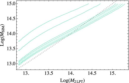
Mapping of masses between 2LPT haloes and N-body haloes as a function of linking length, b, for one realization. From top to bottom linking length are as follows: 0.27, 0.30, 0.36, 0.37, 0.38 (in lighter colour), 0.39 and 0.40. N-body haloes use b − 0.2.

Open in new tab Download slide

Figure 5.

Ratios between PTHalos and N-body halo–matter cross-power spectra as a function of halo mass threshold, for a linking length of b = 0.38 (2LPT) and b = 0.2 (N-body) for one realization. The halo masses are given in Table 1.

Open in new tab Download slide

The mapping between the 2LPT masses and the N-body masses is an essential part of the PTHalos method; without it the PThalos correlation functions would not be close to those from the N-body simulations. In Fig. 4, we show the mapping of the 2LPT and N-body masses for different values of the linking length. We observe that massive haloes have larger masses in the 2LPT field than in the N-body simulation. This is expected, since the typical theoretical size of the 2LPT haloes, as explained in Section 6.1, is about 3.3 times larger than the size of the same halo in the N-body simulation. Consequently, massive haloes, having larger volumes in the 2LPT field, would accrete into themselves the mass of the surrounding filaments and close neighbouring haloes.

We also observe that low-mass haloes have less mass when obtained in the 2LPT field than in the N-body simulation. This is also expected. In the LPT framework some particles (the ones that would have virialized in a halo) are displaced further than they would have been in an N-body simulation. This effect is known as shell crossing. Small virialized haloes are the ones most affected by shell crossing. Because of the extra displacement some of the particles are likely to become unbound to the 2LPT halo and therefore their mass becomes lower in the 2LPT field than in the N-body simulation.

The sample of haloes in Fig. 3, the million most massive haloes, is equivalent to a mass threshold of M = 3.02 × 10¹³ M_⊙ h⁻¹. We are interested now in comparing the clustering with other mass thresholds. In Fig. 5, we show the ratios P_{hm, 2Lpt}/P_{hm, sim} for range of halo mass thresholds, and linking length b = 0.38. The corresponding masses and colours are referenced in Table 1. Each halo sample corresponds to the most massive N haloes in the 2LPT field, where log (N) = 3.5, 4, 4.5, 5, 5.5, 6, 6.5. The corresponding mass of the halo that is in the position N in the mass-ranked list of the N-body simulation is given also in Table 1, together with the corresponding number of particles of that halo. We have found that all these halo samples yield clustering amplitudes that are still within 10 per cent of those calculated from the N-body simulation.

Table 1.

Open in new tab

The number of haloes, their mass and associated colour. Masses of haloes in N-body simulations as a function of their position in the mass-ranked list. That is, given the N most massive haloes in the volume L = (2400 Mpc h⁻¹)³, the lower mass in the sample is M. Masses are from one run of Oriana N-body simulation at z = 0.52 and are given for the linking length of b = 0.2. Masses are in units of 10¹³ M_⊙ h⁻¹ and are not corrected for discreteness effects. For each halo mass we have shown in parentheses the number of particles that halo has given our mass resolution.

log N	Mass (N_part)	Colour
3.5	44.3 (968)	Red
4.0	30.7 (672)	Light green
4.5	19.8 (432)	Blue
5.0	11.7 (256)	Purple
5.5	6.31 (138)	Orange
6.0	3.02 (66)	Cyan
6.5	1.28 (46)	Dark green

Table 1.

Open in new tab

The number of haloes, their mass and associated colour. Masses of haloes in N-body simulations as a function of their position in the mass-ranked list. That is, given the N most massive haloes in the volume L = (2400 Mpc h⁻¹)³, the lower mass in the sample is M. Masses are from one run of Oriana N-body simulation at z = 0.52 and are given for the linking length of b = 0.2. Masses are in units of 10¹³ M_⊙ h⁻¹ and are not corrected for discreteness effects. For each halo mass we have shown in parentheses the number of particles that halo has given our mass resolution.

log N	Mass (N_part)	Colour
3.5	44.3 (968)	Red
4.0	30.7 (672)	Light green
4.5	19.8 (432)	Blue
5.0	11.7 (256)	Purple
5.5	6.31 (138)	Orange
6.0	3.02 (66)	Cyan
6.5	1.28 (46)	Dark green

We note that the ratio between the PThalos clustering and the N-body haloes clustering does not change monotonically with mass. As the mass threshold is lowered, the ratio decreases until a point from which this trend is inverted and the ratio starts to increase. We have no clear understanding of why this is the case. However, we have found that the clustering of the lower mass PThalos increases significantly if the smoothing of the initial power spectrum is not applied, thus increasing the difference with the N-body clustering. This seems to indicate that the FoF algorithm spuriously creates a few number of small haloes near the most massive ones because of the larger density of matter around them. We leave the detailed study of this effect for a future work.

We will use the linking length b = 0.38, which is the theoretical expectation, as our fiducial value in the following sections.

6.3 Variance and cross-correlation coefficients

Having set the PThalos linking length, we run 40 2LPT dark matter fields, with the same Fourier phases and amplitudes as the 40 simulations of LasDamas suite. For all of them we compute the halo–matter cross-power spectra as in the previous section, for the first million haloes of both PThalos and N-body haloes, and we compute the corresponding covariance matrices:

\begin{eqnarray} &&C(k_i,k_j) = \nonumber \\ && \frac{1}{N-1}\sum _{i=1}^{N=40} \left[P^i_{{\rm hm}}(k_1) -\bar{P}_{{\rm hm}}(k_1)\right] \left[P^i_{{\rm hm}}(k_2)-\bar{P}_{{\rm hm}}(k_2)\right] , \end{eqnarray}

(15)

where |$\bar{P}_{{\rm hm}}$| is the mean power spectrum of the set of simulations. The variance of the cross-power spectrum is defined as variance = Var(k) = C(k, k) and the correlation coefficients of a given k₁ as |${\rm Corr}(k_1,k)=C(k_1,k)/\sqrt{{\rm Var}(k_1) {\rm Var} (k)}$|⁠.

In the top panel of Fig. 6, we show the ratio of the variances between PTHalos and N-body simulations, for the first million haloes, which is an equivalent mass threshold of 3.02 × 10¹³ M_⊙ h⁻¹. We can see that most points lie within 15 per cent range of the expected value at linear order, which is given by the square of the ratio of the halo bias. This estimate comes from assuming that the halo–matter cross-power spectrum is proportional to the halo bias, Pⁱ_hm = b_hPⁱ_mm, where Pⁱ_mm indicates the matter power spectrum, and the halo bias, b_h, is independent of the realization. In this approximation the variance is proportional to the square of the bias, consequently the ratio of the variances of 2LPT and N-body simulations is proportional to the ratio of the halo bias. We have computed this ratio using the mean of the halo bias for the 40 realizations. The ratio of one realization has been shown in Figs 3 and 5. Since the bias of the haloes is accurate at 10 per cent, the variance is accurate at about 20 per cent.

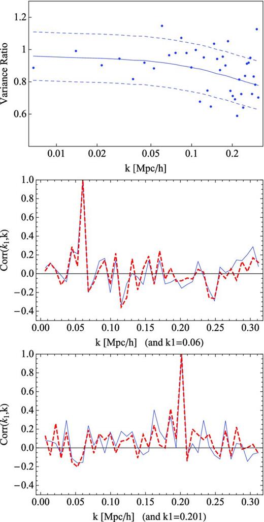
Top: ratio of the cross-power variance of PTHalos and N-body simulations for a mass threshold of 3.02 × 1013 M⊙ h−1. The expected ratio is shown in a solid line and a 15 per cent band range is shown in dashed lines. Middle and bottom: comparison of correlation coefficients of N-body (solid blue) and PTHalos (dashed red) halo–matter cross-power spectra. Middle: k1 = 0.06. Bottom k1 = 0.201.

Figure 6.

Top: ratio of the cross-power variance of PTHalos and N-body simulations for a mass threshold of 3.02 × 10¹³ M_⊙ h⁻¹. The expected ratio is shown in a solid line and a 15 per cent band range is shown in dashed lines. Middle and bottom: comparison of correlation coefficients of N-body (solid blue) and PTHalos (dashed red) halo–matter cross-power spectra. Middle: k₁ = 0.06. Bottom k₁ = 0.201.

Open in new tab Download slide

In the middle and bottom panels of Fig. 6, we show a comparison between the correlation coefficients of PThalos (dashed red) and N-body haloes (solid blue). Each line shows the estimate from the 40 realizations that have the same phases. Both are clearly similar, showing that the PThalos preserve the same structures as the N-body simulations.

6.4 Autocorrelation

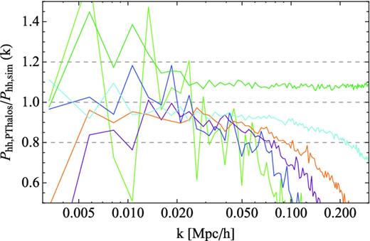
In Fig. 7, we show the ratio between the autopower spectrum of PThalos and the autopower of N-body haloes, where we did not subtract a shot-noise contribution. We see that for all the mass thresholds this ratio is well within 10 per cent. We note that there is not a monotonic relation between the masses and the ratio of the power spectra. Starting with the most massive haloes the ratio decreases as the mass threshold is lowered, but this tendency is reversed for lower mass haloes, as seen, for instance, in the lower mass range (dark green line) in which haloes are more clustered than the N-body haloes of equivalent mass. This reversal could be due to a fraction of small haloes being clustered around massive ones, probably because of the shell-crossing effects that make haloes in 2LPT less compact than in N-body simulations.

Figure 7.

Ratios between PTHalos and N-body halo power spectra as a function of k for different halo mass thresholds, for a linking length of b = 0.38 (2LPT) and b = 0.2 (N-body). Haloes are from one realization with the same phases in each simulation. The correspondence between colour and halo mass thresholds is given in Table 1. The power spectra have not been corrected for shot noise.

Open in new tab Download slide

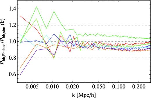
In Fig. 8, we show the ratio of the autopower spectra for one realization of PThalos and one realization of N-body haloes from LasDamas with the same Fourier phases. Before doing the ratio, a Poisson shot-noise contribution of 1/n (where n is the number density of haloes) was subtracted from the power, as is common under the approximation of Poisson sampling. Note, however, that there are indications in the literature that the shot noise of haloes is not strictly Poisson (appendix A, Smith et al. 2008). As seen in Fig. 8 we recover a ratio within ∼20 per cent for most masses and range of scales, which is consistent with our findings of an accuracy of 10 per cent or less in the ratio of the bias (or equivalently of the cross-power spectra). At small scales, for k > 0.15 h Mpc⁻¹, PTHalos performance decreases significantly, and the ratio of powers reaches 20 per cent for some masses. In such cases the expected difference of the variances is 40 per cent. For clarity in Fig. 8 we do not show our results for the lower mass range; they are similar to the haloes with M > 30.7 × 10¹³ M_⊙ h⁻¹ but with a larger scatter that would make difficult to understand the plot if included.

Figure 8.

Same as Fig. 7 but with shot-noise-corrected power spectra, assuming Poisson noise.

Open in new tab Download slide

In Figs 9 and 10 we show the ratio of the autopower spectra for the mean of the 40 realizations of PThalos and an N-body halo, with and without shot-noise correction. We show the results for the first million haloes, which in all realizations correspond to the mass threshold of 3.02 × 10¹³ M_⊙ h⁻¹. Dashed lines show the rms range of this measurement, which is an estimation of the scatter between realizations.

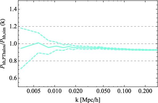
Ratio between PTHalos and N-body halo power spectra as a function of k, for the mean of the 40 realizations, and mass threshold of M = 3.02 × 1013 M⊙ h−1, corresponding to the first million haloes in each realization. Linking length used are b = 0.38 (2LPT) and b = 0.2 (N-body). Dashed lines show the range of the standard deviation. The power spectra have not been corrected for shot noise.

Figure 9.

Ratio between PTHalos and N-body halo power spectra as a function of k, for the mean of the 40 realizations, and mass threshold of M = 3.02 × 10¹³ M_⊙ h⁻¹, corresponding to the first million haloes in each realization. Linking length used are b = 0.38 (2LPT) and b = 0.2 (N-body). Dashed lines show the range of the standard deviation. The power spectra have not been corrected for shot noise.

Open in new tab Download slide

Figure 10.

Same as Fig. 9 but with shot-noise-corrected power spectra, assuming Poisson noise.

Open in new tab Download slide

6.5 PTHalos with WMAP cosmology

So far we have established a method to obtain haloes from a 2LPT dark matter field, which matches the clustering of simulations at 10 per cent. We have tested the method by comparing the clustering of PThalos with that of the haloes from LasDamas N-body simulations suite.

In the rest of this paper, we use our WMAP fiducial cosmology, which is closer to that expected from observations.

Using our PTHalos code we have generated 600 2LPT fields at z = 0.55. PThalos were obtained using a linking length of b = 0.38. Note that because of the change in cosmology and redshift the predicted linking length (see Section 6.1 for details) has changed to b = 0.375. This is only a very small difference with our fiducial value, which, as seen in Section 6.2, only changes the clustering of haloes by a small amount. For these 600 runs, since we cannot use the LasDamas mass function to set the mass of the PThalos we instead use the general description of Tinker et al. (2008), using SO haloes corresponding to 200 times the mean background density. The calibration between 2LPT and PThalos masses using the Tinker et al. (2008) mass function is shown in Fig. 12.

We do not expect the change in cosmological model to significantly affect the accuracy of the PTHalos method. Nonetheless, we have compared the PThalos clustering with the clustering of the N-body simulation of White et al. (2011) for haloes above 10¹³ M_⊙ h⁻¹. This N-body simulation reproduces a piece of the universe with the same cosmological parameters that we use in the remaining of the paper. N-body haloes are identified with a FoF algorithm with b = 0.168, but the clustering is still matched at the 10 per cent level. This can be seen in Fig. 11 where we have plotted the ratio of the halo power spectrum calculated from the N-body simulation and that from the PTHalos method. The ratio looks smoother than in the other figures because having the power spectra evaluated at different keys, we have interpolated the values before taking the ratio. This result in Fig. 11 shows the robustness of the PTHalos method.

Figure 11.

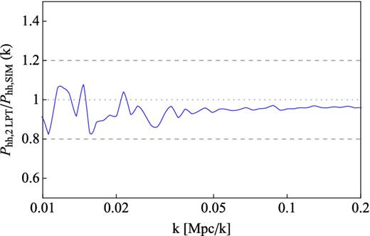
The ratio between the average halo power spectrum calculated from PTHalos simulations and the power spectrum calculated for haloes selected from the White et al. (2011) simulation. For both we apply a mass cut of 10¹³ M_⊙ h⁻¹. Poisson shot noise (1/n) has been subtracted.

Open in new tab Download slide

For this N-body simulation we also show in Fig. 13 the mass function of the haloes together with that of Tinker et al. 2008, which is the mass function we used to set the masses of PThalos for our fiducial WMAP cosmology. As expected the fit is good except at the low-mass end where the mass resolution effects of our simulation start to become important.

Figure 12.

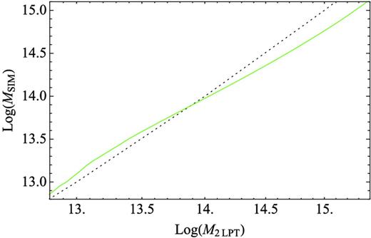
Calibration of mass between 2LPT haloes with WMAP cosmology and haloes that follow Tinker et al. (2008) mass function with the same cosmology (dashed line). The equality relation between the two masses is shown as a dotted line.

Open in new tab Download slide

Figure 13.

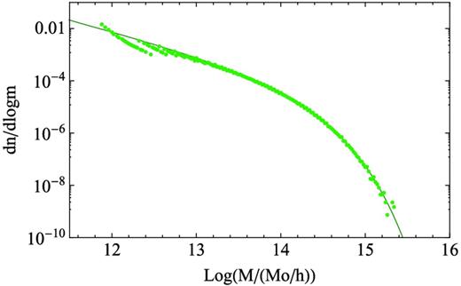
Comparison of mass functions from the simulation of White et al. (2011), assuming a friends-of-friends parameter b = 0.168, and the Tinker et al. (2008) mass-function fitting function for haloes corresponding to 200 times the mean background density.

Open in new tab Download slide

7 POPULATING HALOES WITH GALAXIES

7.1 Halo occupation distribution

To populate haloes with galaxies we use a HOD (Peacock & Smith 2000; Scoccimarro et al. 2001; Berlind & Weinberg 2002) functional form with five parameters, as used by Zheng, Coil & Zehavi (2007). In this form, the mean number of galaxies in a halo of mass M is the sum of the mean number of central galaxies plus the mean number of satellite galaxies, N(M) = 〈N_cen(M)〉 + 〈N_sat(M)〉, where

\begin{eqnarray} \langle N_{{\rm cen}} \rangle &=& \frac{1}{2} \left[ 1 + {{\rm erf}}\left( \frac{{\rm log} M - {\rm log} M_{{\rm min}} }{\sigma _{{\rm log} M}}\right)\right] \nonumber \\ \langle N_{{\rm sat}}\rangle &=& \langle N_{{\rm cen}}\rangle \left( \frac{M - M_0 }{M_1}\right)^\alpha \;, \end{eqnarray}

(16)

and N_sat = 0 if the halo has M < M₀. The error function characterizes the scatter between the mass and the luminosity of the central galaxy, and the power law in the satellite occupation term characterizes the efficiency of galaxy formation on mass. The exact values of the HOD parameters that we use were determined by fitting the DR9 galaxy clustering data, as explained in Section 8.1. The probability of finding a central galaxy in a halo is given by N_cen, and the number of satellites is drawn from a Poisson distribution with mean value N_sat. In the rare event that we draw one satellite galaxy but no central one, we treat it as a central.

7.2 Halo profile

We have distributed satellite galaxies within a halo following an NFW density profile (Navarro, Frenk & White 1996):

\begin{equation} \rho (r) = \frac{4 \rho _s}{\frac{r}{r_s}\left(1+\frac{r}{r_s}\right)^2} \;, \end{equation}

(17)

where r_s is the characteristic radius where the profile has a slope of −2, and ρ_s is the density at this radius. The ratio between the virial radius R_vir and the characteristic radius gives the concentration parameter,

\begin{equation} c = \frac{R_{\rm vir}}{r_s}. \end{equation}

(18)

The masses of the haloes and their concentrations are related. For our galaxy mocks we use the relation found by Prada et al. (2012) when fitting data from N-body simulations:

\begin{eqnarray} c(M,z) &=& \frac{B_0(x)}{B_0(1.393)},\, \mathcal {C}(\sigma ^{\prime }), \nonumber \\ \sigma ^{\prime }&=& \frac{B_1(x)}{B_1(1.393)}\, \sigma (M,x), \nonumber \\ \mathcal {C}(\sigma ^{\prime }) &=& A \, \left[\left(\frac{\sigma ^{\prime }}{b}\right)^c+1\right] \exp \left(\frac{{\rm d}}{\sigma ^{\prime 2}}\right), \end{eqnarray}

(19)

where

\begin{eqnarray} B_0(x) & = & c_0+ (c_1- c_0) \left[\frac{1}{\pi }\arctan \left[\alpha (x-x_0)\right] + \frac{1}{2} \right], \nonumber \\ B_1(x) & = & \frac{1}{\sigma _0}+ \left(\frac{1}{\sigma _1}-\frac{1}{\sigma _0}\right) \left[\frac{1}{\pi }\arctan \left[\beta (x-x_1)\right] +\frac{1}{2} \right], \end{eqnarray}

(20)

and the parameters from the N-body fit are A = 2.881, b = 1.257, c = 1.022, d = 0.060, c₀ = 3.681, c₁ = 5.033, α = 6.948, x₀ = 0.424, σ^{− 1}₀ = 1.047, σ^{− 1}₁ = 1.646, β = 7.386 and x₁ = 0.526.

The cosmology and redshift dependence of the fit enter through |$x=(\Omega _\Lambda /\Omega _{\rm m})^{1/3}/(1+z)$| and through the variance of the haloes of a given mass, σ(M, z). The masses in the equations above are defined such that the mean density at the virial radius is 200 times the critical density, to match the Tinker et al. (2008) definition. Using the NFW we can easily move from one definition of halo mass to another, and use each formula appropriately.

We have added a dispersion to the mass–concentration relation. We use a lognormal distribution; thus the probability of a concentration c for a halo of mass M is

\begin{equation} p(c|M) = \frac{1}{c \sqrt{2\pi \sigma _{\log c}^2}} {{\rm exp}} \left[ -\frac{ { {{\log }}[c/\bar{c}(M,z)] }^2 }{2\sigma _{\log c}^2}\right] \end{equation}

(21)

where |$\bar{c}$| is the mean mass–concentration relation. Typical values of σ_log c are between 0.043 and 0.109 (Giocoli et al. 2010). We have chosen for our mocks the value σ_log c = 0.078, which is close to the mean.

The scatter of the mass–concentration is not dependent on cosmological parameters (Maccio, Dutton & van den Bosch 2008).

7.3 Galaxy velocities in haloes

We assign velocities to the galaxies in haloes by using the virial theorem, which states that the average kinetic energy of particles is half the average of the negative potential energy, 〈v²〉 = 〈GM(r)/r〉. This average over the dark matter particles can be expressed as an integral of dark matter profile:

\begin{equation} \langle v^2 \rangle = \frac{\int _0^R G M(r) \mathrm{d}M}{\int _0^{R_{\rm vir}} \mathrm{d}M}. \end{equation}

(22)

Assuming an NFW profile, the mass inside a given radius is

\begin{equation*} M(r) = \frac{4 \pi }{3}\rho _s^3 \cdot 12\left[ \ln (1+x) - \frac{x}{1+x}\right], \end{equation*}

and therefore, the virial velocity reads

\begin{eqnarray} \langle v^2 \rangle & = & \frac{ G M }{R_{\rm vir}} c \frac{\frac{c}{2(1+c)}-\frac{{\rm ln}(1+c)}{1+c} }{\left[{\rm ln}(1+c)-\frac{c}{1+c}\right]^2} \nonumber \\ &=& \frac{ G M }{R_{\rm vir}}\, c \,\frac{ 0.5\, c (1+c) - (1+c) {\rm ln}(1+c) }{\left[(1+c){\rm ln}(1+c)-c\right]^2} \nonumber \\ &\equiv & \frac{ G M }{R_{\rm vir}} F(c), \end{eqnarray}

(23)

where the last equality defines F(c) that we will use later. Here, again, c denotes the concentration parameter, c = R_vir/r_s, r_s denotes the characteristic NFW radius and R_vir denotes the virial radius, defined as the radius at which the average density of the halo is Δ times the mean density |$\bar{\rho }$|⁠, |$M=4\pi /3 R^3 \Delta \bar{\rho }$|⁠. As mentioned before, the value of Δ is typically taken to be 200, and we use this value in PTHalos, but other numbers are also motivated by the spherical collapse model and N-body simulations.

Once we have the typical velocity dispersion of a halo we assign positions and velocities to its galaxies in the following way. If there is only one galaxy, we place it at the centre of mass with the velocity of the halo. If there is more than one galaxy, the first one is placed at the centre of mass, and the others following the NFW density profile. For these galaxies their velocities have two components: the velocity of the halo centre of mass and a contribution from the velocity dispersion. We take the latter to be drawn from a Gaussian distribution with zero mean and variance equal to

\begin{equation} \big\langle v_{{\rm 1D}}^2 \big\rangle = \frac{1}{3} \big\langle v_x^2+v_y^2+v_z^2 \big\rangle = \frac{1}{3} \langle v^2\rangle . \end{equation}

(24)

7.4 Redshift-space distortions

We use the velocity of galaxies to simulate the effects of RSD. We therefore alter the positions of galaxies such that each galaxy is set to where it would be observed in redshift-space coordinates. To achieve this one must convert velocities into displacements by dividing the former by |$\mathcal {H}=\dot{a}=Ha$| and projecting the result along the line of sight. The displacement Δs in Mpc h⁻¹ that corresponds to a velocity of magnitude of |$\sqrt{\langle v_{{\rm 1D}}^2 \rangle }$| is easily computed. Since G = 3H²₀/8πρ_crit, |$\rho _{{\rm crit}}=\Omega _M^0 \bar{\rho }$|⁠, and defining the Hubble expansion rate as H(z) ≡ H₀E(z), one gets

\begin{equation} \Delta s = \frac{R_{\rm vir}}{E(z)a} \sqrt{F(c)} \;, \end{equation}

(25)

where F(c) has been defined in equation (23). We add the RSD along the line of sight, rather than displacing the galaxies along a single axes, as in the distant observer approximation implementation.

7.4.1 Extending the model

We have made several simplifying assumptions within the method presented in this paper. In particular, many effects of the complex relation between haloes, matter and galaxies are not included in these mock galaxy catalogues.

We choose to model the galaxies on top of a static realization of the matter field, which assumes that the evolution over the redshift range is small. This will impact the clustering of matter, as well as the associated halo masses. Although we expect this effect to be small for the mock galaxy catalogues used in CMASS DR9 results, we could improve on the method for future applications and model this evolution.

For simplicity, the mocks also neglect any evolution to populating dark matter haloes, or varying the galaxy bias with redshift. While the sampling of galaxies is adjusted to match the density as a function of redshift (see Fig. 2), a change in number density is likely to correspond to a variation in galaxy selection, and therefore, the associated galaxy bias (more luminous galaxies typically correspond to lower number densities and higher bias values). Again, we expect a small impact on any CMASS DR9 results (Anderson et al. 2012) since much of the modelling assumes an average bias value over the redshift range, which the galaxy mocks appropriately match.

We also did not include assembly bias effects (Sheth & Tormen 2004; Croft et al. 2011) in our mocks, but kept the concentration parameter and HOD independent of the environment. For simplicity, we also have set independent scatters for the number of galaxies in a halo and the concentration parameter, even if, at a fixed halo mass, they might be related.

Haloes in the mocks are spherical. In reality, as shown by N-body simulations, they have a range of shapes that are correlated to the morphology of the surrounding environment (Smith & Watts 2005 ; White, Cohn & Smith 2010; Schneider, Frenk & Cole 2012). The mocks described in this paper included none of these effects. In future versions, a correlation with the environment could be introduced via the 2LPT estimation of the tidal field.

Finally, the galaxies in the mocks have no individual colours or luminosities. One could include them by following a similar prescription to one described in Skibba et al. (2006) and Skibba & Sheth (2009) which was constrained by SDSS luminosity and colour-dependent clustering, number densities and colour–magnitude distributions.

8 GALAXY MOCKS FOR THE CMASS DR9 SAMPLE

8.1 Fit to CMASS galaxies

In order to find values of HOD parameters we fit the measured clustering of the full BOSS CMASS DR9 sample (NGC plus SGC) with a model based on a mock realization. We choose the mock realization for which the power spectrum is closest to the mean of the mocks and compute, for each HOD iteration, ξ(s) with s between 30 and 80 Mpc h⁻¹, in an area of a quarter of the sky, with a simple mask and a constant n(z), but including RSD. We populate haloes below a minimum mass threshold of M = 0.47 × 10¹³ M_⊙ h⁻¹, which corresponds to haloes of 10 particles. The rest of the galaxies, which according to each HOD would belong to haloes with a lower mass, are placed on randomly selected dark matter particles, of which ∼11 per cent belong to haloes. The χ² is computed in 14 bins in log(r), using the monopole data from Reid et al. (2012), and with a covariance matrix that comes from a previous version of the mocks. By fitting our HOD to the galaxy clustering we are partially compensating for the differences between the clustering of haloes in simulations and the clustering of PThalos.

To find values of HOD parameters that minimize χ² we use the simplex algorithm of Nedler & Mead (1965). We start by making an initial guess about the values of the HOD parameters and then construct a 5D simplex with vertices at this initial point and five other points that resulted from stepping along each coordinate axes with a certain step size. The algorithm finds the vertex with the worst χ² value and moves it by a combination of reflection, reflection followed by expansion and multiple contractions until the value of χ² at that vertex is no longer the worst. The algorithm then keeps contracting the simplex by moving the next worst vertex until the size of the average distance from the centre of the simplex to its vertices is smaller than a desired level of accuracy. If the χ² surface is unimodal this algorithm is guaranteed to find the minimum with any desired accuracy.

Our initial guess of HOD parameters was the best-fitting set computed using the clustering and number density of an earlier CMASS sample (see White et al. 2011). After about 40 steps the resulting best-fitting HOD was

\begin{eqnarray} &&{{\rm log}}(M_{{\rm min}})=13.09,\nonumber \\ &&{{\rm log}}(M_1)=14.00,\nonumber \\ &&{{\rm log}}(M_0)=13.077,\nonumber \\ &&\sigma _{{\rm log}M}=0.596, \nonumber \\ &&\alpha =1.0127. \end{eqnarray}

(26)

We find χ² = 5.89 with nine degrees of freedom. In Fig. 14 we show in black the mean number of galaxies as a function of halo mass for our best fit. In red we show the best-fitting model of White et al. (2011). Both agree to within the 1σ errors, and the mean number of galaxies at a given mass, N(M), agrees better than 10 per cent for haloes below 10^14.5 M_⊙ h⁻¹ and better than 20 per cent between 10^14.5 and 10¹⁵ M_⊙ h⁻¹.

Figure 14.

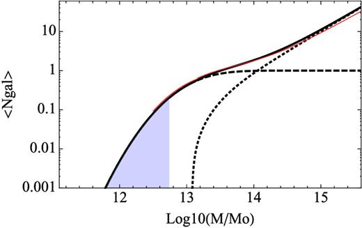
Best-fitting HOD of the mocks (black solid line), with its contribution split between central galaxies (dashed line) and satellite galaxies (dotted line). Grey shadowed area shows the mass range for which galaxies are drawn from matter particles. White et al. (2011) best HOD fit to CMASS data is shown in red.

Open in new tab Download slide

The shadowed area in the plot denotes the masses for which we have no haloes in the simulation. The galaxies corresponding to those haloes have been assigned positions and velocities of randomly selected dark matter particles. They form ∼25 per cent of the total of mock galaxies. If we did not include them then we would not have recovered a sensible HOD because we would have had to populate the available low-mass PThalos with far too many galaxies in order to reduce the bias.

It is possible to set the HOD parameters of the mocks more accurately by fitting both the two-point and the three-point correlation functions, as the latter helps to break degeneracies between the parameters (Sefusatti & Scoccimarro 2005; Kulkarni et al. 2007). However, computing the three-point function in each step of the fitting process is computationally very time consuming. We leave this improvement as a possibility for future versions of the mocks.

8.2 Geometry and mask

We wish to create mocks with a geometry appropriate for the BOSS CMASS DR9 galaxy sample, including both the NGC and the SGC, with redshifts between 0.43 and 0.7. These are the data used in a number of recent cosmological analyses (Anderson et al. 2012; Nuza et al. 2012; Reid et al. 2012; Ross et al. 2012; Sánchez et al. 2012; Tojeiro et al. 2012a,b; Samushia et al. 2012). In this section we show how we match the DR9 CMASS geometry.

The NGC and SGC regions can individually be fitted into a reshaped box with size L = 2.4 Gpc h⁻¹, which is the size we adopted for our PTHalos runs. The reshaping is achieved as follows: starting with a cubic box of size L, we cut the xy plane as indicated in the top panel of Fig. 15. Using the periodicity of the PTHalos simulation we can copy or move the particles from outside the range L/2 < x + y < 3L/2 into that same range. Thus, as shown in the second panel from the top of Fig. 15, we can obtain a rectangular box of size |${{L}}/\sqrt{2},2{{L}}/\sqrt{2},{{L}}$|⁠. The last dimension is defined as the z-direction. This technique is similar to volume remapping of Carlson & White (2010).

Figure 15.

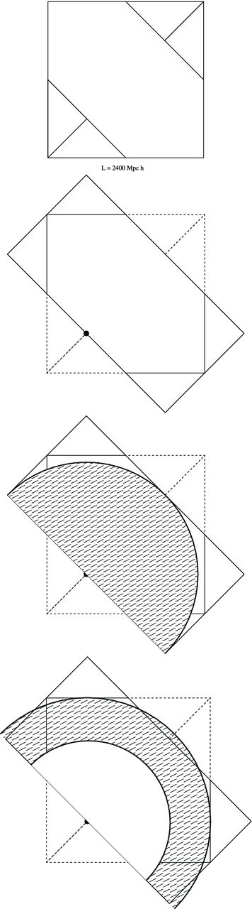
Procedure to fit the geometry of DR9 into the simulation box using periodic boundary conditions. See text for details.

Open in new tab Download slide

With this geometry, placing our observer at (x, y, z) = (L/4, L/4, 0) we can cover a quarter of the sky up to a distance of |${{L}}/\sqrt{2}$| from the observer without repetition of the underlying matter distribution. This is shown in the third panel from the top of Fig. 15. For the WMAP cosmological model this distance is equivalent to reaching a redshift z = 0.663. Note, however, that the constraint of a maximum distance of |${{L}}/\sqrt{2}$| is set only because of the geometry of the z = 0 plane. Keeping the observer in the same place, but looking into a direction off the plane, we could map to a higher distance without repeating the sampled volumes. Translating to consider an angular region, the above maximum distance is only valid if we require a full 180° wide view and, for example, an opening of 126| ${.\!\!\!\!\!\!^{\circ}}$|87 centred on the direction |$\hat{\boldsymbol e}=(\hat{\boldsymbol x}+\hat{\boldsymbol y})/\sqrt{2}$| would allow us to reach a distance of |$\sqrt{5/8}{{L}}$| without repetition. The actual maximum distance achievable with any given box without repetition will depend on the angular mask of the survey being analysed.

To generate the mocks for DR9 CMASS, we first produce a redshift shell such as that shown in the bottom panel of Fig. 15. We then rotate the 3D coordinates to fit either the NGC or SGC angular footprint into the box containing the redshift shell. Images of these angular footprints are shown in Fig. 1. The extent of these masks means that our boxes are of sufficient size that mock catalogues containing galaxies with redshifts z < 0.7 do not suffer from any repetition of the underlying density field.

In order to mimic the observations as closely as possible, we use the mangle software (Swanson et al. 2008) to differentiate between sectors that have different observational properties, as described in Ross et al. (2012). The completeness in the mock galaxies is defined slightly differently from that of the CMASS DR9 catalogues. As we are only interested in large scales, we do not mimic the full small-scale BOSS targeting procedure in the mocks. In particular, we ignore the effect of missing close pairs of galaxies that result from the fact that we cannot observe two targets closer than 62 arcsec with the same plate; this is a physical limitation imposed by the size of the fibres. We also ignore the effect of plate-scale angular variations in our redshift success rate. In section 3 of Anderson et al. (2012) two completeness measures are defined: the fraction of objects targeted that are observed or are in a close pair, C_BOSS, and the fraction of galaxies with good redshifts, C_red. For the mocks, we revise the definition of sector completeness such the angular variations in galaxy density follow those in the sample with good redshifts, ignoring close pairs. We therefore define

\begin{equation} C_{\rm mock}=\frac{N_{\rm obs}}{N_{\rm targ}-N_{\rm known}}, \end{equation}

(27)

where N_obs is the number of objects observed spectroscopically by BOSS in any sector, N_targ is the number of target objects and N_known is the number that already have good-quality known redshifts. Following Anderson et al. (2012), the redshift completeness is defined as

\begin{equation} C_{\rm red}=\frac{N_{\rm gal}}{N_{\rm obs}-N_{\rm star}}, \end{equation}

(28)

where N_gal is the number of targets within a sector, observed by BOSS and subsequently spectroscopically classified as galaxies with good redshifts, and N_star is the number classified as stars. We subsample galaxies in our mock catalogues based on the product C_mock × C_red, i.e. we subsample based on angular fluctuations of galaxies with good redshifts, ignoring other subtleties. The implemented angular mask can be seen in Fig. 1.

As we are only interested in matching the large-scale clustering signal we do not include small-scale holes in the survey mask such as those due to SDSS fields with known photometric problems, objects observed with higher priorities, bright stars and plate centres (see Anderson et al. 2012 for details). In total these remove 5 per cent of the mask area, as defined by overlapping tiles, and the holes represent small angular patches that are approximately randomly distributed. As we are only interested in large scales, the net effect on removing such holes is equivalent to reducing the galaxy density, rather than the volume. Consequently, we simply match the total galaxy number after removing these regions from the CMASS DR9 galaxy catalogue.

In order to mimic the measured redshift distribution we subsample the galaxies in each PTHalos mock based on a smooth fit to the measured redshift distribution, n(z). We do this separately for the NGC and SGC areas, as they have slightly different redshift distributions (see Fig. 2; Ross et al. 2012).

Using the above procedure we generated 600 PTHalos mocks with WMAP underlying cosmology, for both NGC and SGC areas. Note that the volumes sampled in NGC mock i and SCG mock i will partially overlap, where 1 < i < 600 refers to the mask number.

9 RESULTS FROM THE CMASS DR9 MOCKS

9.1 Correlation function monopole

We have used the Landy & Szalay (1993) estimator to calculate the anisotropic redshift-space correlation function, ξ(s, μ), where s is the redshift-space separation and μ is the cosine of the angle between the galaxy pair and the line of sight:

\begin{equation} \xi (s,\mu ) = \frac{DD(s,\mu )-2DR(s,\mu )}{RR(s,\mu )}+1 \;, \end{equation}

(29)

where D stands for the data number counts and R stands for the random sample number counts with the same redshift distribution and angular footprint as the data sample.

The moments of ξ(s, μ), expanded in Legendre polynomials, contain all of the information about the correlation function. They are given by

\begin{equation} \xi _{\ell }(s) = \frac{(2\ell + 1)}{2}\int _{-1}^{1} \xi (s,\mu ) P_{\ell }(\mu ) {\rm d}\mu . \end{equation}

(30)

We will focus on the monopole ξ₀ and the quadrupole ξ₂ (see below) as in linear theory they contain most of the information. We weight pair counts based on their number density, with weights w = (1 + n(z)P_fkp)^{− 1} (Feldman, Kaiser & Peacock 1994), where P_fkp = 20000 h^{− 3} Mpc³. The same applies to the power spectrum. For more details on the weighting see Ross et al. (2012) and Anderson et al. (2012).

In the top panel of Fig. 16 we present the mean of the monopole of the correlation function ξ₀(s) from our mocks. The red and blue lines show the mean of the 600 mocks using the NGC and SGC footprint, respectively. The two means are similar as expected, and differ only because of cosmic variance and differences in the survey geometry. The error bars show the rms of the mocks, and thus give an estimation of the typical dispersion between them. The errors are smaller for the NGC because of the larger area. The DR9 CMASS ξ₀(s) is shown as open circles.

Figure 16.

Top: correlation function monopole ξ(s) of the NGC and SGC mocks, respectively, shown in red and blue. The NGC footprint having larger area has smaller errors. CMASS DR9 data are shown in open circles. Error bars are from the 600 galaxy mock catalogues. Bottom: the relative bias between the mocks and the data, shown for the NGC mocks.

Open in new tab Download slide

The relative bias between the data and the mean of the NGC mocks is shown in the bottom panel of Fig. 16. The differences between data and mocks are consistent within the data errors on the scales plotted.

In the top panel of Fig. 17 we present the distributions of the values of the correlation function of the mocks for several separation distances, in normalized units. That is, for each bin in s of the correlation function ξ(s) one can compute its variance and express the value of the correlation function in its units. The histogram of the 600 values is also normalized to one. Thus if the mocks are Gaussian this distribution should follow a normalized Gaussian distribution. In red solid lines we show the results for the NGC sample, and in blue dashed lines the results for the SGC sample. We see no significant deviation from the Gaussian distribution shown in black dotted lines, and there is no particular scale appearing to perform worse than the others.

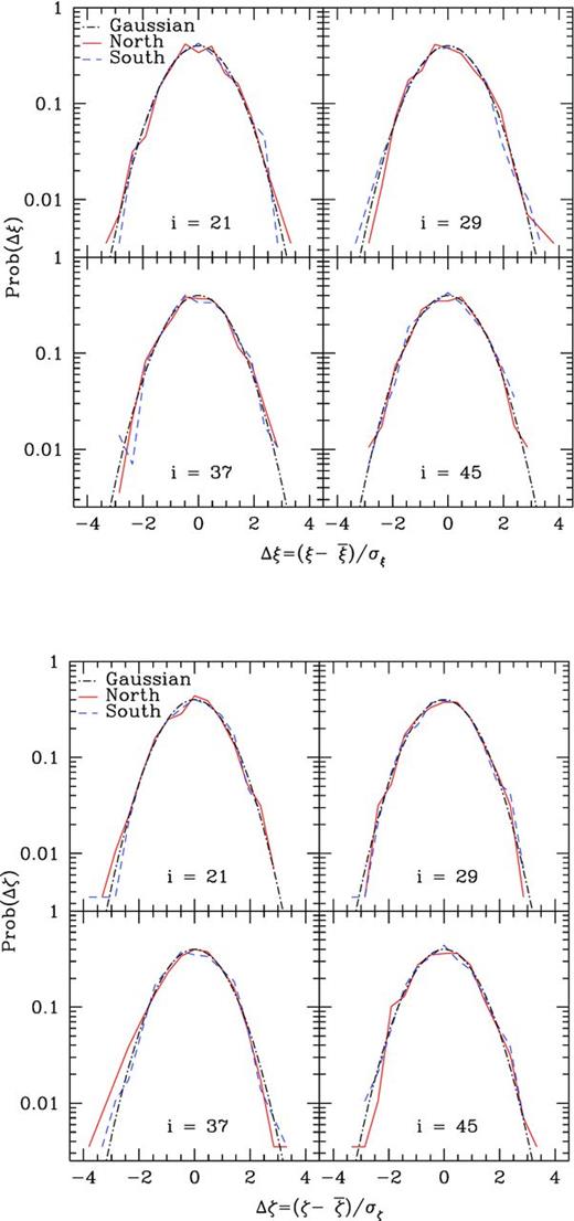
Top: histogram of the normalized residual counts of the correlation function ξ(s) for scales s = 84, 116, 148 and 180 Mpc h−1, corresponding to our bins i = 21, 29, 37 and 45. Bottom: histogram of the normalized residual counts of the correlation function ξ(s) after being projected into the space where the covariance is diagonal, ζi, in the bins i = 21, 29, 37 and 45. Each bin now has contributions from all scales (see main text).

Figure 17.

Top: histogram of the normalized residual counts of the correlation function ξ(s) for scales s = 84, 116, 148 and 180 Mpc h⁻¹, corresponding to our bins i = 21, 29, 37 and 45. Bottom: histogram of the normalized residual counts of the correlation function ξ(s) after being projected into the space where the covariance is diagonal, ζ_i, in the bins i = 21, 29, 37 and 45. Each bin now has contributions from all scales (see main text).

Open in new tab Download slide

The values of the correlation functions at different scales are correlated. To have a better understanding of their distribution we have made a transformation of the correlation function into the basis where the covariance matrix is diagonal. This is, we have computed ζ_j ≡ M_{i, j}ξ_i, where ξ_i is the correlation function at bin i and M is the matrix constituted by the eigenvectors of the correlation function ordered by their eigenvalues. In the bottom panel of Fig. 17, we show the normalized distributions of the projected correlation functions ζ_i, for different bins. Each bin has contribution from all scales, but, in this basis, the distribution of values in each bin is independent of the others. In red solid lines we show the results for the NGC sample, and in blue dashed lines the results of the SGC sample. We see no significant deviation from the Gaussian distribution shown in black dotted lines, and, again, there is no particular scale appearing to perform worse than the others.

To check the compatibility of the distribution of the mocks with a Gaussian distribution, we performed a Kolmogorov–Smirnov test on the measured distribution function of ξ_t(s) of the NGC sample. The result depends on the range of scales used. For scales in the range of 50 < s < 150 Mpc h⁻¹, in 9 per cent of the cases, a sample drawn from a Gaussian distribution with zero mean and unit variance would appear less Gaussian than that the distribution obtained from the 600 mocks.

9.2 Correlation function quadrupole

In Fig. 18, we show the average measurement of the quadrupole for the NGC (red) and SGC (blue) mocks. The quadrupole measured from the CMASS DR9 data is shown by the open circles. Error bars show the rms of the 600 mocks. The anisotropic clustering, i.e. the quadrupole, can be used to estimate the growth rate of structure f.

Top: correlation function quadrupole ξ2(s) of the NGC and SGC mocks, respectively, shown in red and blue. The NGC footprint having larger area has smaller errors. CMASS DR9 data are shown in open circles. Error bars show the rms of 600 galaxy mock catalogues. Bottom: the relative bias between the mocks and the data, shown for the NGC mocks.

Figure 18.

Top: correlation function quadrupole ξ₂(s) of the NGC and SGC mocks, respectively, shown in red and blue. The NGC footprint having larger area has smaller errors. CMASS DR9 data are shown in open circles. Error bars show the rms of 600 galaxy mock catalogues. Bottom: the relative bias between the mocks and the data, shown for the NGC mocks.

Open in new tab Download slide

In the linear regime the expression for the RSD is (Hamilton 1992)

\begin{equation} \xi _0(s) = \left(b_{\rm g}^2+\frac{2}{3}b_{\rm g}f+\frac{1}{5}f^2\right)\xi ^{\rm r}(s)\;, \end{equation}

(31)

\begin{equation} \xi _2(s) = -\left(\frac{4}{3} b_{\rm g} f +\frac{4}{7} f^2 \right)\left[\bar{\xi }(s) - \xi ^{\rm r}(s)\right]\;, \end{equation}

(32)

where ξ^r is the real-space matter correlation function normalized so that

\begin{equation} \displaystyle \int _0^\infty \xi ^{\rm r}(s)s^2{\rm d}s=1 , \end{equation}

(33)

|$\bar{\xi }$| is given by

\begin{equation} \bar{\xi }(s) = \frac{3}{s^3}\displaystyle \int _0^s \xi ^{\rm r}(s^{\prime })s^{\prime 2}{\rm d}s^{\prime }, \end{equation}

(34)

and b_g is the bias of galaxies.

We have estimated values of galaxy bias b_g and growth rate f in the mocks by performing a joint fit to the measured redshift-space monopole and quadrupole of the correlation function within scales of 50 < s < 150 Mpc h⁻¹. We used the standard perturbation theory predictions of the real-space pairwise halo velocity statistics to model the non-linear contribution to the redshift-space correlation function (Reid & White 2011). The fit gives b_g = 1.90 and f = 0.729. The value of the growth rate recovered in this fit is very close to the value from linear theory for our cosmological parameters, f = 0.744 (only a 2 per cent difference).

Note that if we were to fit the quadrupole of the correlation function using only the linear theory to model the shape of the multipoles and the linear Kaiser formula for RSD (equation 32), then the recovered best value of the fit to f would be lower. This is expected due to non-linearities, which act to decrease the redshift-space anisotropies predicted by the Kaiser formula, even on relatively large scales (Scoccimarro 2004).

9.3 Power spectrum

The top panel of Fig. 19 shows the average power spectrum of the mocks, both for the NGC and SGC footprints, compared with the DR9 CMASS galaxy power spectrum. In the bottom panel we show the relative bias between the data and the mocks, i.e. the square root of the ratio between their respective power spectra. The relative bias is within 10 per cent for scales in the range of 0.01 < k < 0.2 and increases at very low k.

Figure 19.

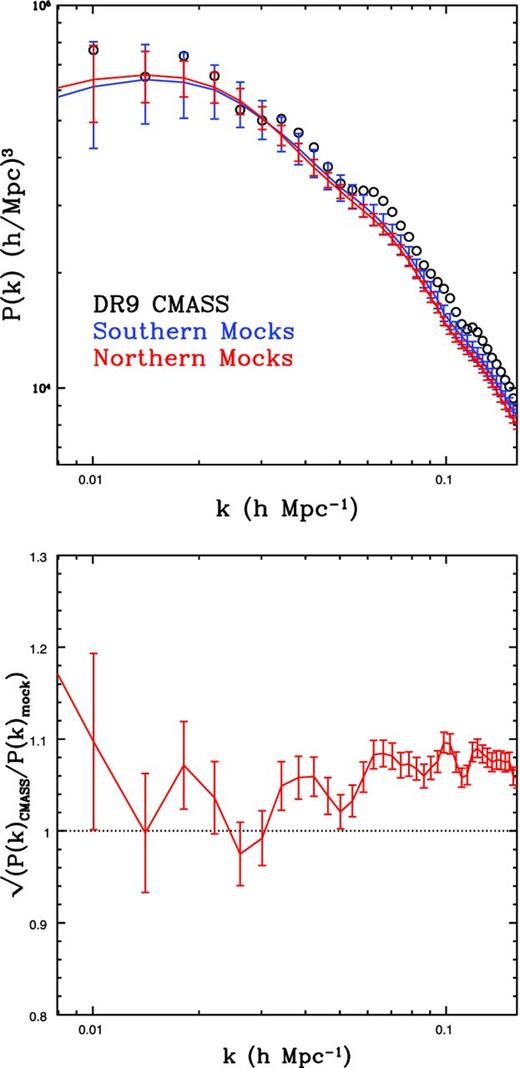
Top: power spectrum P(k) of the NGC and SGC mocks, respectively, shown in red and blue. CMASS DR9 data are shown in open circles. Error bars are from the 600 galaxy mock catalogues. Bottom: relative bias between the mocks and the data, shown for the NGC mocks. The NGC footprint has the smaller errors because of its larger area.

Open in new tab Download slide

The amplitude of the power spectrum of the data is slightly higher than the average of the mocks. Consequently, the mocks underestimate the errors of the amplitude of the measured power spectrum by the same factor, as the sample limit is proportional to the power spectrum amplitude.

10 COMPARISON WITH ANALYTIC PREDICTION

In this section we compare the covariance matrix of the galaxy mocks described above to a covariance matrix based on the analytical approach of de Putter et al. (2012). This approach provides a prescription for the dark matter power spectrum covariance matrix, taking into account the effects of survey geometry and using standard perturbation theory to include non-linear effects. The resulting covariance matrix has been shown to agree well with N-body simulations for modes k < 0.2 h Mpc⁻¹. However, to analytically describe the covariance matrix of the galaxy two-point function, the effects of galaxy bias, RSD and shot noise need to be taken into account in addition to the dark matter prescription. We now describe our simplified assumptions for these ingredients below.

Galaxy bias is assumed to be linear and scale independent, with a value of b_g = 1.9, which is the best fit to the mocks. Shot noise due to the finite number of galaxies is incorporated following Feldman, Kaiser & Peacock (FKP, 1994), which treats the shot noise as Gaussian. Finally, RSD are incorporated using the expression based on linear theory and the plane-parallel approximation (Kaiser 1987) |$\delta _{\rm g}({\boldsymbol k}) \rightarrow [1 + \beta (\hat{\boldsymbol k} \cdot \hat{\boldsymbol n})^2] \, \delta _{\rm g}({\boldsymbol k})$|⁠, where β = f/b_g, with f ≡ dln d/dln a ≈ Ω^0.55_m(z) the growth factor and |$\hat{\boldsymbol n}$| the line-of-sight unit vector. On large scales, this causes a simple rescaling of the covariance matrix by the angle average of the fourth power of the ‘Kaiser factor’, a_rsd(β) ≡ 1 + 4/3β + 6/5β² + 4/7β³ + 1/9β⁴, which we use to multiply the entire covariance matrix.

The final analytic model for the covariance between galaxy power spectrum estimators in bins i and j in k-space is obtained by symmetrizing

\begin{eqnarray} {\boldsymbol c}_{ij}^{\rm gal} &=& \left[ 2 \int _i \frac{{\rm d}^3 {\boldsymbol k}}{v_{k,i}} \, \int _j \frac{{\rm d}^3 {\boldsymbol k^{\prime }}}{v_{k,j}} \, \big|b_{\rm g}^2 \, p(k) \, q({\boldsymbol k} - {\boldsymbol k^{\prime }}) + s({\boldsymbol k} - {\boldsymbol k^{\prime }})\big|^2 \right. \nonumber \\ &&\left. + \, b_{\rm g}^4 \, {\boldsymbol c}_{ij}^{\rm matt, non{\rm -}lin} \right] \times a_{\rm rsd}(\beta ), \end{eqnarray}

(35)

where v_{k, i} is the k-volume in a bin i, p(k) is the matter power spectrum, and

\begin{equation} q({\boldsymbol k}) \equiv {I_{22}({\boldsymbol k})\over I_{22}({\boldsymbol 0})}, \ \ \ \ \ s({\boldsymbol k}) \equiv {I_{12}({\boldsymbol k})\over I_{22}({\boldsymbol 0})}, \end{equation}

(36)

with |$I_{ij}({\boldsymbol k}) = \int \bar{n}^i({\boldsymbol r}) w^j({\boldsymbol r}) {\rm e}^{{\rm i} {\boldsymbol k}\cdot {\boldsymbol r}} {\rm d}^3 r$|⁠, |$\bar{n}$| the selection function of the survey and |$w=(1+\bar{n} P_0)^{-1}$| the optimal FKP weight function. In equation (35), |${\boldsymbol c}_{ij}^{\rm matt, non{\rm -}lin}$| describes the non-Gaussian matter power spectrum covariance matrix and is given by the second and third lines of equation (47) in de Putter et al. (2012), to which we refer the reader for more details.

To obtain the covariance matrix of the two-point function, this matrix is transformed applying the linear transformation between the Feldman et al. (1994) power spectrum estimator and the Landy & Szalay (1993) correlation function estimator.

The main caveats in the analytic method come from the simplified transformation described above between the real-space dark matter covariance matrix and the redshift-space galaxy covariance matrix. In reality, the galaxy bias is not linear and this affects the non-Gaussian contribution to the covariance matrix. Moreover, the analytic model only describes RSD at the linear level, and therefore does not include ‘fingers of god’ effects which appear already on weakly non-linear scales. Finally, the shot noise also contributes to the non-Gaussian part of the covariance matrix. However, the analytic description is expected to work well in the linear regime, and provides a reasonable estimate to compare to the numerical method from the mocks in the range of scales of interest (35–140 Mpc h⁻¹).

We now compare the galaxy mock covariance matrix with the analytic estimates using the DR9 NGC footprint and assuming our WMAP fiducial cosmology described in Section 5.

We start first with the power spectrum covariance matrix. Fig. 20 shows the normalized (to have unit diagonal) covariance matrix or cross-correlation coefficients, C(k₁, k), of the power spectrum of the mocks (in solid blue lines) and of the analytical model (in red dashed lines). The plots are for the values of k = 0.0624 and 0.204 h Mpc⁻¹ but similar results are obtained when fixing k₁ at other values. The mocks have a somewhat stronger correlation amplitude than the analytical model, which is not surprising given that non-linear contributions from RSD and bias are not taken into account in equation (35), as discussed above.

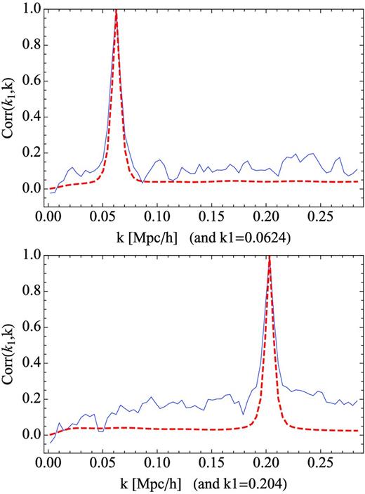
Correlation coefficients C(k, k1) for the power spectrum of the mocks (in blue solid lines) compared to the analytical values (in dashed red lines).

Figure 20.

Correlation coefficients C(k, k₁) for the power spectrum of the mocks (in blue solid lines) compared to the analytical values (in dashed red lines).

Open in new tab Download slide

We now turn to configuration space. Fig. 21 shows the ratio between the analytical values of the variance of the correlation function and the values from the variance of the mocks, which differ less than 10 per cent. Fig. 22 shows the eigenvalues from the mock correlation functions (blue circles) compared with the eigenvalues of the analytical model (red squares). Both give comparable results, largest eigenvalues having differences at the ≲10 per cent level, which increases up to 25 per cent for the fourteenth eigenvalue.

Figure 21.

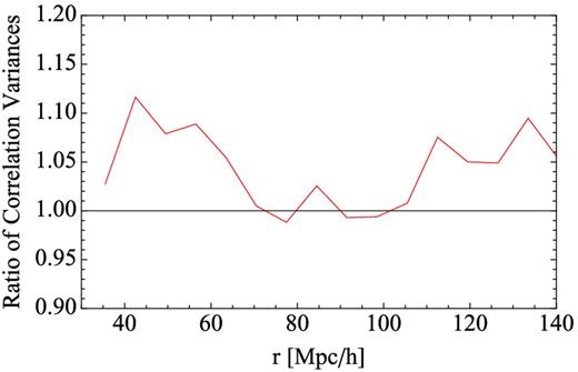
Comparison of the values of the variance of the correlation function of the mocks as a function of scale with the analytical value of the de Putter et al. (2012). The plot shows the ratio of the analytical value against the mocks.

Open in new tab Download slide

Figure 22.

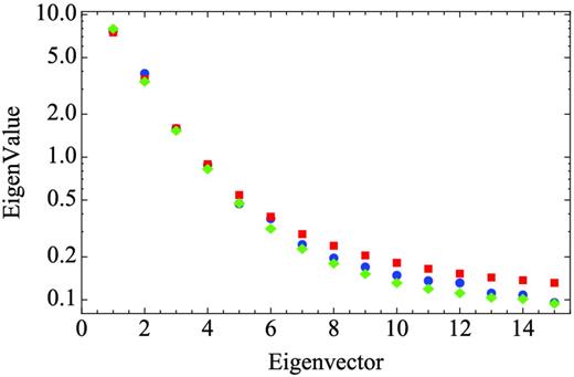
Eigenvalues of the normalized covariance matrix of the mocks’ correlation function (blue circles) compared to an smoothed version of it (green diamonds) and to analytical values (red squares).

Open in new tab Download slide

Fig. 22 also shows a comparison with the method of Xu et al. (2012), denoted by green diamonds, which is based on fitting a modified form of the Gaussian covariance matrix to the sample covariance matrix from the mocks using a maximum likelihood approach. The eigenvalues of the smoothed version of the covariance matrix are consistent at the 10 per cent level with the values of the sample covariance from the mocks.

11 CORRELATION FUNCTION AND COVARIANCE MATRIX TABLES

Tables 2 and 3 show, respectively, the mean monopole correlation function and the covariance matrix of the 600 mocks each, each for both the NGC and SGC footprints. The logarithmic binning of the correlation function adopted matches that of Samushia et al. (2012) and Reid et al. (2012).

Table 2.

Open in new tab

The monopole of the correlation function multiplied by 10⁵, for ξ₀(s) with 30 < s < 160 h⁻¹ Mpc for the DR9 NGC and SGC mocks. Correlation functions from PTHalos galaxy mock catalogues will be available with this and other binnings will be available at ‘http://www.marcmanera.net/mocks/’.

s Mpc/h	30.8	33.4	36.2	39.2	42.5	46.1	49.9	54.1	58.7	63.6	68.9	74.7	81.0	87.8	95.1
ξ₀(s) NGC	497.07	408.22	333.79	270.19	216.45	171.90	134.90	104.60	79.56	59.34	43.06	30.87	22.05	17.49	18.11
ξ₀(s) SGC	484.07	397.71	322.96	261.15	207.05	163.71	127.21	96.39	72.85	53.02	37.46	25.43	17.12	12.90	13.25
s Mpc/h	103.1	111.8	121.1	131.3	142.3	154.3
ξ₀(s) NGC	19.39	15.45	6.84	−0.45	−3.77	−4.43
ξ₀(s) SGC	15.59	12.36	4.23	−2.83	−6.02	−6.20

s Mpc/h	30.8	33.4	36.2	39.2	42.5	46.1	49.9	54.1	58.7	63.6	68.9	74.7	81.0	87.8	95.1
ξ₀(s) NGC	497.07	408.22	333.79	270.19	216.45	171.90	134.90	104.60	79.56	59.34	43.06	30.87	22.05	17.49	18.11
ξ₀(s) SGC	484.07	397.71	322.96	261.15	207.05	163.71	127.21	96.39	72.85	53.02	37.46	25.43	17.12	12.90	13.25
s Mpc/h	103.1	111.8	121.1	131.3	142.3	154.3
ξ₀(s) NGC	19.39	15.45	6.84	−0.45	−3.77	−4.43
ξ₀(s) SGC	15.59	12.36	4.23	−2.83	−6.02	−6.20

Table 2.

Open in new tab

The monopole of the correlation function multiplied by 10⁵, for ξ₀(s) with 30 < s < 160 h⁻¹ Mpc for the DR9 NGC and SGC mocks. Correlation functions from PTHalos galaxy mock catalogues will be available with this and other binnings will be available at ‘http://www.marcmanera.net/mocks/’.

s Mpc/h	30.8	33.4	36.2	39.2	42.5	46.1	49.9	54.1	58.7	63.6	68.9	74.7	81.0	87.8	95.1
ξ₀(s) NGC	497.07	408.22	333.79	270.19	216.45	171.90	134.90	104.60	79.56	59.34	43.06	30.87	22.05	17.49	18.11
ξ₀(s) SGC	484.07	397.71	322.96	261.15	207.05	163.71	127.21	96.39	72.85	53.02	37.46	25.43	17.12	12.90	13.25
s Mpc/h	103.1	111.8	121.1	131.3	142.3	154.3
ξ₀(s) NGC	19.39	15.45	6.84	−0.45	−3.77	−4.43
ξ₀(s) SGC	15.59	12.36	4.23	−2.83	−6.02	−6.20

s Mpc/h	30.8	33.4	36.2	39.2	42.5	46.1	49.9	54.1	58.7	63.6	68.9	74.7	81.0	87.8	95.1
ξ₀(s) NGC	497.07	408.22	333.79	270.19	216.45	171.90	134.90	104.60	79.56	59.34	43.06	30.87	22.05	17.49	18.11
ξ₀(s) SGC	484.07	397.71	322.96	261.15	207.05	163.71	127.21	96.39	72.85	53.02	37.46	25.43	17.12	12.90	13.25
s Mpc/h	103.1	111.8	121.1	131.3	142.3	154.3
ξ₀(s) NGC	19.39	15.45	6.84	−0.45	−3.77	−4.43
ξ₀(s) SGC	15.59	12.36	4.23	−2.83	−6.02	−6.20

Table 3.

Open in new tab

The covariance matrix, multiplied by 10⁵, for ξ₀(s) with 30 < s < 160 h⁻¹ Mpc, for the DR9 NGC (top) and SGC (bottom) footprint. Covariance matrices from PTHalos galaxy mock catalogues with this and other binnings will be available at ‘http://www.marcmanera.net/mocks/’.

s Mpc/h	30.8	33.4	36.2	39.2	42.5	46.1	49.9	54.1	58.7	63.6	68.9	74.7	81.0	87.8	95.1	103.1	111.8	121.1	131.3	142.3	154.3
30.7	2.11	1.51	1.37	1.20	1.05	0.89	0.78	0.65	0.52	0.50	0.40	0.31	0.26	0.21	0.18	0.14	0.10	0.06	0.03	0.01	−0.01
33.3	1.51	1.71	1.29	1.15	1.00	0.86	0.75	0.64	0.51	0.49	0.41	0.31	0.26	0.20	0.16	0.13	0.09	0.05	0.02	−0.00	−0.01
36.1	1.37	1.29	1.50	1.12	0.98	0.84	0.75	0.64	0.53	0.48	0.43	0.33	0.28	0.23	0.19	0.15	0.11	0.08	0.06	0.03	0.01
39.1	1.20	1.15	1.12	1.27	0.96	0.84	0.73	0.61	0.52	0.49	0.44	0.32	0.28	0.23	0.19	0.16	0.12	0.09	0.06	0.03	0.01
42.4	1.05	1.00	0.98	0.96	1.10	0.85	0.74	0.64	0.56	0.52	0.44	0.35	0.30	0.25	0.22	0.18	0.14	0.09	0.06	0.05	0.02
46.0	0.89	0.86	0.84	0.84	0.85	0.96	0.72	0.64	0.55	0.50	0.43	0.34	0.30	0.25	0.21	0.18	0.13	0.09	0.06	0.04	0.02
49.8	0.78	0.75	0.75	0.73	0.74	0.72	0.81	0.64	0.57	0.52	0.46	0.38	0.32	0.27	0.23	0.19	0.15	0.11	0.08	0.06	0.04
54.0	0.65	0.64	0.64	0.61	0.64	0.64	0.64	0.71	0.56	0.51	0.43	0.36	0.31	0.26	0.22	0.18	0.14	0.11	0.07	0.06	0.05
58.5	0.52	0.51	0.53	0.52	0.56	0.55	0.57	0.56	0.64	0.53	0.46	0.38	0.33	0.27	0.24	0.19	0.16	0.12	0.10	0.08	0.06
63.5	0.50	0.49	0.48	0.49	0.52	0.50	0.52	0.51	0.53	0.59	0.49	0.41	0.36	0.30	0.26	0.21	0.17	0.12	0.10	0.08	0.07
68.8	0.40	0.41	0.43	0.44	0.44	0.43	0.46	0.43	0.46	0.49	0.54	0.44	0.38	0.33	0.28	0.23	0.18	0.13	0.11	0.09	0.08
74.6	0.31	0.31	0.33	0.32	0.35	0.34	0.38	0.36	0.38	0.41	0.44	0.47	0.39	0.33	0.28	0.23	0.18	0.13	0.11	0.08	0.08
80.8	0.26	0.26	0.28	0.28	0.30	0.30	0.32	0.31	0.33	0.36	0.38	0.39	0.42	0.35	0.30	0.25	0.20	0.16	0.13	0.10	0.09
87.6	0.21	0.20	0.23	0.23	0.25	0.25	0.27	0.26	0.27	0.30	0.33	0.33	0.35	0.38	0.33	0.28	0.22	0.17	0.14	0.11	0.10
95.0	0.18	0.16	0.19	0.19	0.22	0.21	0.23	0.22	0.24	0.26	0.28	0.28	0.30	0.33	0.36	0.30	0.25	0.19	0.16	0.13	0.10
102.9	0.14	0.13	0.15	0.16	0.18	0.18	0.19	0.18	0.19	0.21	0.23	0.23	0.25	0.28	0.30	0.31	0.26	0.20	0.17	0.14	0.11
111.6	0.10	0.09	0.11	0.12	0.14	0.13	0.15	0.14	0.16	0.17	0.18	0.18	0.20	0.22	0.25	0.26	0.27	0.22	0.18	0.15	0.12
120.9	0.06	0.05	0.08	0.09	0.09	0.09	0.11	0.11	0.12	0.12	0.13	0.13	0.16	0.17	0.19	0.20	0.22	0.23	0.19	0.15	0.12
131.1	0.03	0.02	0.06	0.06	0.06	0.06	0.08	0.07	0.10	0.10	0.11	0.11	0.13	0.14	0.16	0.17	0.18	0.19	0.21	0.17	0.14
142.1	0.01	−0.00	0.03	0.03	0.05	0.04	0.06	0.06	0.08	0.08	0.09	0.08	0.10	0.11	0.13	0.14	0.15	0.15	0.17	0.19	0.16

154.0	−0.01	−0.01	0.01	0.01	0.02	0.02	0.04	0.05	0.06	0.07	0.08	0.08	0.09	0.10	0.10	0.11	0.12	0.12	0.14	0.16	0.18
\|$\vphantom{{}^{A^A}}$\|s Mpc/h	30.7	33.3	36.1	39.1	42.4	46.0	49.8	54.0	58.5	63.5	68.8	74.6	80.8	87.6	95.0	102.9	111.6	120.9	131.1	142.1	154.0
30.7	6.80	5.11	4.36	3.95	3.31	2.94	2.57	2.08	1.75	1.36	1.19	0.83	0.74	0.64	0.63	0.46	0.33	0.27	0.24	0.15	0.08
33.3	5.11	6.11	4.44	3.87	3.40	3.12	2.79	2.25	1.87	1.48	1.22	0.91	0.79	0.69	0.60	0.46	0.38	0.30	0.28	0.22	0.14
36.1	4.36	4.44	5.08	3.88	3.42	3.03	2.65	2.18	1.83	1.43	1.17	0.91	0.78	0.70	0.59	0.46	0.42	0.34	0.30	0.24	0.19
39.1	3.95	3.87	3.88	4.46	3.51	3.07	2.66	2.23	1.89	1.49	1.16	0.92	0.77	0.68	0.57	0.43	0.34	0.31	0.26	0.20	0.17
42.4	3.31	3.40	3.42	3.51	4.06	3.18	2.77	2.30	1.95	1.48	1.20	1.00	0.85	0.70	0.58	0.46	0.38	0.32	0.29	0.20	0.17
46.0	2.94	3.12	3.03	3.07	3.18	3.70	2.92	2.46	2.04	1.65	1.42	1.17	0.93	0.81	0.63	0.46	0.39	0.33	0.30	0.21	0.18
49.8	2.57	2.79	2.65	2.66	2.77	2.92	3.24	2.45	2.09	1.70	1.44	1.18	0.99	0.83	0.67	0.50	0.41	0.34	0.31	0.24	0.21
54.0	2.08	2.25	2.18	2.23	2.30	2.46	2.45	2.76	2.14	1.77	1.48	1.21	1.00	0.83	0.65	0.52	0.43	0.39	0.37	0.29	0.24
58.5	1.75	1.87	1.83	1.89	1.95	2.04	2.09	2.14	2.36	1.83	1.53	1.23	1.06	0.87	0.69	0.55	0.44	0.40	0.36	0.29	0.26
63.5	1.36	1.48	1.43	1.49	1.48	1.65	1.70	1.77	1.83	1.99	1.58	1.28	1.11	0.92	0.77	0.64	0.50	0.47	0.42	0.33	0.28
68.8	1.19	1.22	1.17	1.16	1.20	1.42	1.44	1.48	1.53	1.58	1.80	1.39	1.17	0.98	0.80	0.65	0.52	0.46	0.42	0.33	0.27
74.6	0.83	0.91	0.91	0.92	1.00	1.17	1.18	1.21	1.23	1.28	1.39	1.52	1.21	1.00	0.81	0.66	0.51	0.42	0.39	0.31	0.25
80.8	0.74	0.79	0.78	0.77	0.85	0.93	0.99	1.00	1.06	1.11	1.17	1.21	1.36	1.12	0.91	0.76	0.60	0.49	0.43	0.36	0.30
87.6	0.64	0.69	0.70	0.68	0.70	0.81	0.83	0.83	0.87	0.92	0.98	1.00	1.12	1.29	1.04	0.88	0.71	0.58	0.48	0.40	0.34
95.0	0.63	0.60	0.59	0.57	0.58	0.63	0.67	0.65	0.69	0.77	0.80	0.81	0.91	1.04	1.16	0.98	0.82	0.66	0.55	0.45	0.38
102.9	0.46	0.46	0.46	0.43	0.46	0.46	0.50	0.52	0.55	0.64	0.65	0.66	0.76	0.88	0.98	1.11	0.92	0.75	0.63	0.51	0.44
111.6	0.33	0.38	0.42	0.34	0.38	0.39	0.41	0.43	0.44	0.50	0.52	0.51	0.60	0.71	0.82	0.92	1.03	0.83	0.69	0.56	0.47
120.9	0.27	0.30	0.34	0.31	0.32	0.33	0.34	0.39	0.40	0.47	0.46	0.42	0.49	0.58	0.66	0.75	0.83	0.88	0.74	0.59	0.48
131.1	0.24	0.28	0.30	0.26	0.29	0.30	0.31	0.37	0.36	0.42	0.42	0.39	0.43	0.48	0.55	0.63	0.69	0.74	0.84	0.69	0.56
142.1	0.15	0.22	0.24	0.20	0.20	0.21	0.24	0.29	0.29	0.33	0.33	0.31	0.36	0.40	0.45	0.51	0.56	0.59	0.69	0.74	0.62
154.0	0.08	0.14	0.19	0.17	0.17	0.18	0.21	0.24	0.26	0.28	0.27	0.25	0.30	0.34	0.38	0.44	0.47	0.48	0.56	0.62	0.72

s Mpc/h	30.8	33.4	36.2	39.2	42.5	46.1	49.9	54.1	58.7	63.6	68.9	74.7	81.0	87.8	95.1	103.1	111.8	121.1	131.3	142.3	154.3
30.7	2.11	1.51	1.37	1.20	1.05	0.89	0.78	0.65	0.52	0.50	0.40	0.31	0.26	0.21	0.18	0.14	0.10	0.06	0.03	0.01	−0.01
33.3	1.51	1.71	1.29	1.15	1.00	0.86	0.75	0.64	0.51	0.49	0.41	0.31	0.26	0.20	0.16	0.13	0.09	0.05	0.02	−0.00	−0.01
36.1	1.37	1.29	1.50	1.12	0.98	0.84	0.75	0.64	0.53	0.48	0.43	0.33	0.28	0.23	0.19	0.15	0.11	0.08	0.06	0.03	0.01
39.1	1.20	1.15	1.12	1.27	0.96	0.84	0.73	0.61	0.52	0.49	0.44	0.32	0.28	0.23	0.19	0.16	0.12	0.09	0.06	0.03	0.01
42.4	1.05	1.00	0.98	0.96	1.10	0.85	0.74	0.64	0.56	0.52	0.44	0.35	0.30	0.25	0.22	0.18	0.14	0.09	0.06	0.05	0.02
46.0	0.89	0.86	0.84	0.84	0.85	0.96	0.72	0.64	0.55	0.50	0.43	0.34	0.30	0.25	0.21	0.18	0.13	0.09	0.06	0.04	0.02
49.8	0.78	0.75	0.75	0.73	0.74	0.72	0.81	0.64	0.57	0.52	0.46	0.38	0.32	0.27	0.23	0.19	0.15	0.11	0.08	0.06	0.04
54.0	0.65	0.64	0.64	0.61	0.64	0.64	0.64	0.71	0.56	0.51	0.43	0.36	0.31	0.26	0.22	0.18	0.14	0.11	0.07	0.06	0.05
58.5	0.52	0.51	0.53	0.52	0.56	0.55	0.57	0.56	0.64	0.53	0.46	0.38	0.33	0.27	0.24	0.19	0.16	0.12	0.10	0.08	0.06
63.5	0.50	0.49	0.48	0.49	0.52	0.50	0.52	0.51	0.53	0.59	0.49	0.41	0.36	0.30	0.26	0.21	0.17	0.12	0.10	0.08	0.07
68.8	0.40	0.41	0.43	0.44	0.44	0.43	0.46	0.43	0.46	0.49	0.54	0.44	0.38	0.33	0.28	0.23	0.18	0.13	0.11	0.09	0.08
74.6	0.31	0.31	0.33	0.32	0.35	0.34	0.38	0.36	0.38	0.41	0.44	0.47	0.39	0.33	0.28	0.23	0.18	0.13	0.11	0.08	0.08
80.8	0.26	0.26	0.28	0.28	0.30	0.30	0.32	0.31	0.33	0.36	0.38	0.39	0.42	0.35	0.30	0.25	0.20	0.16	0.13	0.10	0.09
87.6	0.21	0.20	0.23	0.23	0.25	0.25	0.27	0.26	0.27	0.30	0.33	0.33	0.35	0.38	0.33	0.28	0.22	0.17	0.14	0.11	0.10
95.0	0.18	0.16	0.19	0.19	0.22	0.21	0.23	0.22	0.24	0.26	0.28	0.28	0.30	0.33	0.36	0.30	0.25	0.19	0.16	0.13	0.10
102.9	0.14	0.13	0.15	0.16	0.18	0.18	0.19	0.18	0.19	0.21	0.23	0.23	0.25	0.28	0.30	0.31	0.26	0.20	0.17	0.14	0.11
111.6	0.10	0.09	0.11	0.12	0.14	0.13	0.15	0.14	0.16	0.17	0.18	0.18	0.20	0.22	0.25	0.26	0.27	0.22	0.18	0.15	0.12
120.9	0.06	0.05	0.08	0.09	0.09	0.09	0.11	0.11	0.12	0.12	0.13	0.13	0.16	0.17	0.19	0.20	0.22	0.23	0.19	0.15	0.12
131.1	0.03	0.02	0.06	0.06	0.06	0.06	0.08	0.07	0.10	0.10	0.11	0.11	0.13	0.14	0.16	0.17	0.18	0.19	0.21	0.17	0.14
142.1	0.01	−0.00	0.03	0.03	0.05	0.04	0.06	0.06	0.08	0.08	0.09	0.08	0.10	0.11	0.13	0.14	0.15	0.15	0.17	0.19	0.16

154.0	−0.01	−0.01	0.01	0.01	0.02	0.02	0.04	0.05	0.06	0.07	0.08	0.08	0.09	0.10	0.10	0.11	0.12	0.12	0.14	0.16	0.18
\|$\vphantom{{}^{A^A}}$\|s Mpc/h	30.7	33.3	36.1	39.1	42.4	46.0	49.8	54.0	58.5	63.5	68.8	74.6	80.8	87.6	95.0	102.9	111.6	120.9	131.1	142.1	154.0
30.7	6.80	5.11	4.36	3.95	3.31	2.94	2.57	2.08	1.75	1.36	1.19	0.83	0.74	0.64	0.63	0.46	0.33	0.27	0.24	0.15	0.08
33.3	5.11	6.11	4.44	3.87	3.40	3.12	2.79	2.25	1.87	1.48	1.22	0.91	0.79	0.69	0.60	0.46	0.38	0.30	0.28	0.22	0.14
36.1	4.36	4.44	5.08	3.88	3.42	3.03	2.65	2.18	1.83	1.43	1.17	0.91	0.78	0.70	0.59	0.46	0.42	0.34	0.30	0.24	0.19
39.1	3.95	3.87	3.88	4.46	3.51	3.07	2.66	2.23	1.89	1.49	1.16	0.92	0.77	0.68	0.57	0.43	0.34	0.31	0.26	0.20	0.17
42.4	3.31	3.40	3.42	3.51	4.06	3.18	2.77	2.30	1.95	1.48	1.20	1.00	0.85	0.70	0.58	0.46	0.38	0.32	0.29	0.20	0.17
46.0	2.94	3.12	3.03	3.07	3.18	3.70	2.92	2.46	2.04	1.65	1.42	1.17	0.93	0.81	0.63	0.46	0.39	0.33	0.30	0.21	0.18
49.8	2.57	2.79	2.65	2.66	2.77	2.92	3.24	2.45	2.09	1.70	1.44	1.18	0.99	0.83	0.67	0.50	0.41	0.34	0.31	0.24	0.21
54.0	2.08	2.25	2.18	2.23	2.30	2.46	2.45	2.76	2.14	1.77	1.48	1.21	1.00	0.83	0.65	0.52	0.43	0.39	0.37	0.29	0.24
58.5	1.75	1.87	1.83	1.89	1.95	2.04	2.09	2.14	2.36	1.83	1.53	1.23	1.06	0.87	0.69	0.55	0.44	0.40	0.36	0.29	0.26
63.5	1.36	1.48	1.43	1.49	1.48	1.65	1.70	1.77	1.83	1.99	1.58	1.28	1.11	0.92	0.77	0.64	0.50	0.47	0.42	0.33	0.28
68.8	1.19	1.22	1.17	1.16	1.20	1.42	1.44	1.48	1.53	1.58	1.80	1.39	1.17	0.98	0.80	0.65	0.52	0.46	0.42	0.33	0.27
74.6	0.83	0.91	0.91	0.92	1.00	1.17	1.18	1.21	1.23	1.28	1.39	1.52	1.21	1.00	0.81	0.66	0.51	0.42	0.39	0.31	0.25
80.8	0.74	0.79	0.78	0.77	0.85	0.93	0.99	1.00	1.06	1.11	1.17	1.21	1.36	1.12	0.91	0.76	0.60	0.49	0.43	0.36	0.30
87.6	0.64	0.69	0.70	0.68	0.70	0.81	0.83	0.83	0.87	0.92	0.98	1.00	1.12	1.29	1.04	0.88	0.71	0.58	0.48	0.40	0.34
95.0	0.63	0.60	0.59	0.57	0.58	0.63	0.67	0.65	0.69	0.77	0.80	0.81	0.91	1.04	1.16	0.98	0.82	0.66	0.55	0.45	0.38
102.9	0.46	0.46	0.46	0.43	0.46	0.46	0.50	0.52	0.55	0.64	0.65	0.66	0.76	0.88	0.98	1.11	0.92	0.75	0.63	0.51	0.44
111.6	0.33	0.38	0.42	0.34	0.38	0.39	0.41	0.43	0.44	0.50	0.52	0.51	0.60	0.71	0.82	0.92	1.03	0.83	0.69	0.56	0.47
120.9	0.27	0.30	0.34	0.31	0.32	0.33	0.34	0.39	0.40	0.47	0.46	0.42	0.49	0.58	0.66	0.75	0.83	0.88	0.74	0.59	0.48
131.1	0.24	0.28	0.30	0.26	0.29	0.30	0.31	0.37	0.36	0.42	0.42	0.39	0.43	0.48	0.55	0.63	0.69	0.74	0.84	0.69	0.56
142.1	0.15	0.22	0.24	0.20	0.20	0.21	0.24	0.29	0.29	0.33	0.33	0.31	0.36	0.40	0.45	0.51	0.56	0.59	0.69	0.74	0.62
154.0	0.08	0.14	0.19	0.17	0.17	0.18	0.21	0.24	0.26	0.28	0.27	0.25	0.30	0.34	0.38	0.44	0.47	0.48	0.56	0.62	0.72

Table 3.

Open in new tab

The covariance matrix, multiplied by 10⁵, for ξ₀(s) with 30 < s < 160 h⁻¹ Mpc, for the DR9 NGC (top) and SGC (bottom) footprint. Covariance matrices from PTHalos galaxy mock catalogues with this and other binnings will be available at ‘http://www.marcmanera.net/mocks/’.

s Mpc/h	30.8	33.4	36.2	39.2	42.5	46.1	49.9	54.1	58.7	63.6	68.9	74.7	81.0	87.8	95.1	103.1	111.8	121.1	131.3	142.3	154.3
30.7	2.11	1.51	1.37	1.20	1.05	0.89	0.78	0.65	0.52	0.50	0.40	0.31	0.26	0.21	0.18	0.14	0.10	0.06	0.03	0.01	−0.01
33.3	1.51	1.71	1.29	1.15	1.00	0.86	0.75	0.64	0.51	0.49	0.41	0.31	0.26	0.20	0.16	0.13	0.09	0.05	0.02	−0.00	−0.01
36.1	1.37	1.29	1.50	1.12	0.98	0.84	0.75	0.64	0.53	0.48	0.43	0.33	0.28	0.23	0.19	0.15	0.11	0.08	0.06	0.03	0.01
39.1	1.20	1.15	1.12	1.27	0.96	0.84	0.73	0.61	0.52	0.49	0.44	0.32	0.28	0.23	0.19	0.16	0.12	0.09	0.06	0.03	0.01
42.4	1.05	1.00	0.98	0.96	1.10	0.85	0.74	0.64	0.56	0.52	0.44	0.35	0.30	0.25	0.22	0.18	0.14	0.09	0.06	0.05	0.02
46.0	0.89	0.86	0.84	0.84	0.85	0.96	0.72	0.64	0.55	0.50	0.43	0.34	0.30	0.25	0.21	0.18	0.13	0.09	0.06	0.04	0.02
49.8	0.78	0.75	0.75	0.73	0.74	0.72	0.81	0.64	0.57	0.52	0.46	0.38	0.32	0.27	0.23	0.19	0.15	0.11	0.08	0.06	0.04
54.0	0.65	0.64	0.64	0.61	0.64	0.64	0.64	0.71	0.56	0.51	0.43	0.36	0.31	0.26	0.22	0.18	0.14	0.11	0.07	0.06	0.05
58.5	0.52	0.51	0.53	0.52	0.56	0.55	0.57	0.56	0.64	0.53	0.46	0.38	0.33	0.27	0.24	0.19	0.16	0.12	0.10	0.08	0.06
63.5	0.50	0.49	0.48	0.49	0.52	0.50	0.52	0.51	0.53	0.59	0.49	0.41	0.36	0.30	0.26	0.21	0.17	0.12	0.10	0.08	0.07
68.8	0.40	0.41	0.43	0.44	0.44	0.43	0.46	0.43	0.46	0.49	0.54	0.44	0.38	0.33	0.28	0.23	0.18	0.13	0.11	0.09	0.08
74.6	0.31	0.31	0.33	0.32	0.35	0.34	0.38	0.36	0.38	0.41	0.44	0.47	0.39	0.33	0.28	0.23	0.18	0.13	0.11	0.08	0.08
80.8	0.26	0.26	0.28	0.28	0.30	0.30	0.32	0.31	0.33	0.36	0.38	0.39	0.42	0.35	0.30	0.25	0.20	0.16	0.13	0.10	0.09
87.6	0.21	0.20	0.23	0.23	0.25	0.25	0.27	0.26	0.27	0.30	0.33	0.33	0.35	0.38	0.33	0.28	0.22	0.17	0.14	0.11	0.10
95.0	0.18	0.16	0.19	0.19	0.22	0.21	0.23	0.22	0.24	0.26	0.28	0.28	0.30	0.33	0.36	0.30	0.25	0.19	0.16	0.13	0.10
102.9	0.14	0.13	0.15	0.16	0.18	0.18	0.19	0.18	0.19	0.21	0.23	0.23	0.25	0.28	0.30	0.31	0.26	0.20	0.17	0.14	0.11
111.6	0.10	0.09	0.11	0.12	0.14	0.13	0.15	0.14	0.16	0.17	0.18	0.18	0.20	0.22	0.25	0.26	0.27	0.22	0.18	0.15	0.12
120.9	0.06	0.05	0.08	0.09	0.09	0.09	0.11	0.11	0.12	0.12	0.13	0.13	0.16	0.17	0.19	0.20	0.22	0.23	0.19	0.15	0.12
131.1	0.03	0.02	0.06	0.06	0.06	0.06	0.08	0.07	0.10	0.10	0.11	0.11	0.13	0.14	0.16	0.17	0.18	0.19	0.21	0.17	0.14
142.1	0.01	−0.00	0.03	0.03	0.05	0.04	0.06	0.06	0.08	0.08	0.09	0.08	0.10	0.11	0.13	0.14	0.15	0.15	0.17	0.19	0.16

154.0	−0.01	−0.01	0.01	0.01	0.02	0.02	0.04	0.05	0.06	0.07	0.08	0.08	0.09	0.10	0.10	0.11	0.12	0.12	0.14	0.16	0.18
\|$\vphantom{{}^{A^A}}$\|s Mpc/h	30.7	33.3	36.1	39.1	42.4	46.0	49.8	54.0	58.5	63.5	68.8	74.6	80.8	87.6	95.0	102.9	111.6	120.9	131.1	142.1	154.0
30.7	6.80	5.11	4.36	3.95	3.31	2.94	2.57	2.08	1.75	1.36	1.19	0.83	0.74	0.64	0.63	0.46	0.33	0.27	0.24	0.15	0.08
33.3	5.11	6.11	4.44	3.87	3.40	3.12	2.79	2.25	1.87	1.48	1.22	0.91	0.79	0.69	0.60	0.46	0.38	0.30	0.28	0.22	0.14
36.1	4.36	4.44	5.08	3.88	3.42	3.03	2.65	2.18	1.83	1.43	1.17	0.91	0.78	0.70	0.59	0.46	0.42	0.34	0.30	0.24	0.19
39.1	3.95	3.87	3.88	4.46	3.51	3.07	2.66	2.23	1.89	1.49	1.16	0.92	0.77	0.68	0.57	0.43	0.34	0.31	0.26	0.20	0.17
42.4	3.31	3.40	3.42	3.51	4.06	3.18	2.77	2.30	1.95	1.48	1.20	1.00	0.85	0.70	0.58	0.46	0.38	0.32	0.29	0.20	0.17
46.0	2.94	3.12	3.03	3.07	3.18	3.70	2.92	2.46	2.04	1.65	1.42	1.17	0.93	0.81	0.63	0.46	0.39	0.33	0.30	0.21	0.18
49.8	2.57	2.79	2.65	2.66	2.77	2.92	3.24	2.45	2.09	1.70	1.44	1.18	0.99	0.83	0.67	0.50	0.41	0.34	0.31	0.24	0.21
54.0	2.08	2.25	2.18	2.23	2.30	2.46	2.45	2.76	2.14	1.77	1.48	1.21	1.00	0.83	0.65	0.52	0.43	0.39	0.37	0.29	0.24
58.5	1.75	1.87	1.83	1.89	1.95	2.04	2.09	2.14	2.36	1.83	1.53	1.23	1.06	0.87	0.69	0.55	0.44	0.40	0.36	0.29	0.26
63.5	1.36	1.48	1.43	1.49	1.48	1.65	1.70	1.77	1.83	1.99	1.58	1.28	1.11	0.92	0.77	0.64	0.50	0.47	0.42	0.33	0.28
68.8	1.19	1.22	1.17	1.16	1.20	1.42	1.44	1.48	1.53	1.58	1.80	1.39	1.17	0.98	0.80	0.65	0.52	0.46	0.42	0.33	0.27
74.6	0.83	0.91	0.91	0.92	1.00	1.17	1.18	1.21	1.23	1.28	1.39	1.52	1.21	1.00	0.81	0.66	0.51	0.42	0.39	0.31	0.25
80.8	0.74	0.79	0.78	0.77	0.85	0.93	0.99	1.00	1.06	1.11	1.17	1.21	1.36	1.12	0.91	0.76	0.60	0.49	0.43	0.36	0.30
87.6	0.64	0.69	0.70	0.68	0.70	0.81	0.83	0.83	0.87	0.92	0.98	1.00	1.12	1.29	1.04	0.88	0.71	0.58	0.48	0.40	0.34
95.0	0.63	0.60	0.59	0.57	0.58	0.63	0.67	0.65	0.69	0.77	0.80	0.81	0.91	1.04	1.16	0.98	0.82	0.66	0.55	0.45	0.38
102.9	0.46	0.46	0.46	0.43	0.46	0.46	0.50	0.52	0.55	0.64	0.65	0.66	0.76	0.88	0.98	1.11	0.92	0.75	0.63	0.51	0.44
111.6	0.33	0.38	0.42	0.34	0.38	0.39	0.41	0.43	0.44	0.50	0.52	0.51	0.60	0.71	0.82	0.92	1.03	0.83	0.69	0.56	0.47
120.9	0.27	0.30	0.34	0.31	0.32	0.33	0.34	0.39	0.40	0.47	0.46	0.42	0.49	0.58	0.66	0.75	0.83	0.88	0.74	0.59	0.48
131.1	0.24	0.28	0.30	0.26	0.29	0.30	0.31	0.37	0.36	0.42	0.42	0.39	0.43	0.48	0.55	0.63	0.69	0.74	0.84	0.69	0.56
142.1	0.15	0.22	0.24	0.20	0.20	0.21	0.24	0.29	0.29	0.33	0.33	0.31	0.36	0.40	0.45	0.51	0.56	0.59	0.69	0.74	0.62
154.0	0.08	0.14	0.19	0.17	0.17	0.18	0.21	0.24	0.26	0.28	0.27	0.25	0.30	0.34	0.38	0.44	0.47	0.48	0.56	0.62	0.72

s Mpc/h	30.8	33.4	36.2	39.2	42.5	46.1	49.9	54.1	58.7	63.6	68.9	74.7	81.0	87.8	95.1	103.1	111.8	121.1	131.3	142.3	154.3
30.7	2.11	1.51	1.37	1.20	1.05	0.89	0.78	0.65	0.52	0.50	0.40	0.31	0.26	0.21	0.18	0.14	0.10	0.06	0.03	0.01	−0.01
33.3	1.51	1.71	1.29	1.15	1.00	0.86	0.75	0.64	0.51	0.49	0.41	0.31	0.26	0.20	0.16	0.13	0.09	0.05	0.02	−0.00	−0.01
36.1	1.37	1.29	1.50	1.12	0.98	0.84	0.75	0.64	0.53	0.48	0.43	0.33	0.28	0.23	0.19	0.15	0.11	0.08	0.06	0.03	0.01
39.1	1.20	1.15	1.12	1.27	0.96	0.84	0.73	0.61	0.52	0.49	0.44	0.32	0.28	0.23	0.19	0.16	0.12	0.09	0.06	0.03	0.01
42.4	1.05	1.00	0.98	0.96	1.10	0.85	0.74	0.64	0.56	0.52	0.44	0.35	0.30	0.25	0.22	0.18	0.14	0.09	0.06	0.05	0.02
46.0	0.89	0.86	0.84	0.84	0.85	0.96	0.72	0.64	0.55	0.50	0.43	0.34	0.30	0.25	0.21	0.18	0.13	0.09	0.06	0.04	0.02
49.8	0.78	0.75	0.75	0.73	0.74	0.72	0.81	0.64	0.57	0.52	0.46	0.38	0.32	0.27	0.23	0.19	0.15	0.11	0.08	0.06	0.04
54.0	0.65	0.64	0.64	0.61	0.64	0.64	0.64	0.71	0.56	0.51	0.43	0.36	0.31	0.26	0.22	0.18	0.14	0.11	0.07	0.06	0.05
58.5	0.52	0.51	0.53	0.52	0.56	0.55	0.57	0.56	0.64	0.53	0.46	0.38	0.33	0.27	0.24	0.19	0.16	0.12	0.10	0.08	0.06
63.5	0.50	0.49	0.48	0.49	0.52	0.50	0.52	0.51	0.53	0.59	0.49	0.41	0.36	0.30	0.26	0.21	0.17	0.12	0.10	0.08	0.07
68.8	0.40	0.41	0.43	0.44	0.44	0.43	0.46	0.43	0.46	0.49	0.54	0.44	0.38	0.33	0.28	0.23	0.18	0.13	0.11	0.09	0.08
74.6	0.31	0.31	0.33	0.32	0.35	0.34	0.38	0.36	0.38	0.41	0.44	0.47	0.39	0.33	0.28	0.23	0.18	0.13	0.11	0.08	0.08
80.8	0.26	0.26	0.28	0.28	0.30	0.30	0.32	0.31	0.33	0.36	0.38	0.39	0.42	0.35	0.30	0.25	0.20	0.16	0.13	0.10	0.09
87.6	0.21	0.20	0.23	0.23	0.25	0.25	0.27	0.26	0.27	0.30	0.33	0.33	0.35	0.38	0.33	0.28	0.22	0.17	0.14	0.11	0.10
95.0	0.18	0.16	0.19	0.19	0.22	0.21	0.23	0.22	0.24	0.26	0.28	0.28	0.30	0.33	0.36	0.30	0.25	0.19	0.16	0.13	0.10
102.9	0.14	0.13	0.15	0.16	0.18	0.18	0.19	0.18	0.19	0.21	0.23	0.23	0.25	0.28	0.30	0.31	0.26	0.20	0.17	0.14	0.11
111.6	0.10	0.09	0.11	0.12	0.14	0.13	0.15	0.14	0.16	0.17	0.18	0.18	0.20	0.22	0.25	0.26	0.27	0.22	0.18	0.15	0.12
120.9	0.06	0.05	0.08	0.09	0.09	0.09	0.11	0.11	0.12	0.12	0.13	0.13	0.16	0.17	0.19	0.20	0.22	0.23	0.19	0.15	0.12
131.1	0.03	0.02	0.06	0.06	0.06	0.06	0.08	0.07	0.10	0.10	0.11	0.11	0.13	0.14	0.16	0.17	0.18	0.19	0.21	0.17	0.14
142.1	0.01	−0.00	0.03	0.03	0.05	0.04	0.06	0.06	0.08	0.08	0.09	0.08	0.10	0.11	0.13	0.14	0.15	0.15	0.17	0.19	0.16

154.0	−0.01	−0.01	0.01	0.01	0.02	0.02	0.04	0.05	0.06	0.07	0.08	0.08	0.09	0.10	0.10	0.11	0.12	0.12	0.14	0.16	0.18
\|$\vphantom{{}^{A^A}}$\|s Mpc/h	30.7	33.3	36.1	39.1	42.4	46.0	49.8	54.0	58.5	63.5	68.8	74.6	80.8	87.6	95.0	102.9	111.6	120.9	131.1	142.1	154.0
30.7	6.80	5.11	4.36	3.95	3.31	2.94	2.57	2.08	1.75	1.36	1.19	0.83	0.74	0.64	0.63	0.46	0.33	0.27	0.24	0.15	0.08
33.3	5.11	6.11	4.44	3.87	3.40	3.12	2.79	2.25	1.87	1.48	1.22	0.91	0.79	0.69	0.60	0.46	0.38	0.30	0.28	0.22	0.14
36.1	4.36	4.44	5.08	3.88	3.42	3.03	2.65	2.18	1.83	1.43	1.17	0.91	0.78	0.70	0.59	0.46	0.42	0.34	0.30	0.24	0.19
39.1	3.95	3.87	3.88	4.46	3.51	3.07	2.66	2.23	1.89	1.49	1.16	0.92	0.77	0.68	0.57	0.43	0.34	0.31	0.26	0.20	0.17
42.4	3.31	3.40	3.42	3.51	4.06	3.18	2.77	2.30	1.95	1.48	1.20	1.00	0.85	0.70	0.58	0.46	0.38	0.32	0.29	0.20	0.17
46.0	2.94	3.12	3.03	3.07	3.18	3.70	2.92	2.46	2.04	1.65	1.42	1.17	0.93	0.81	0.63	0.46	0.39	0.33	0.30	0.21	0.18
49.8	2.57	2.79	2.65	2.66	2.77	2.92	3.24	2.45	2.09	1.70	1.44	1.18	0.99	0.83	0.67	0.50	0.41	0.34	0.31	0.24	0.21
54.0	2.08	2.25	2.18	2.23	2.30	2.46	2.45	2.76	2.14	1.77	1.48	1.21	1.00	0.83	0.65	0.52	0.43	0.39	0.37	0.29	0.24
58.5	1.75	1.87	1.83	1.89	1.95	2.04	2.09	2.14	2.36	1.83	1.53	1.23	1.06	0.87	0.69	0.55	0.44	0.40	0.36	0.29	0.26
63.5	1.36	1.48	1.43	1.49	1.48	1.65	1.70	1.77	1.83	1.99	1.58	1.28	1.11	0.92	0.77	0.64	0.50	0.47	0.42	0.33	0.28
68.8	1.19	1.22	1.17	1.16	1.20	1.42	1.44	1.48	1.53	1.58	1.80	1.39	1.17	0.98	0.80	0.65	0.52	0.46	0.42	0.33	0.27
74.6	0.83	0.91	0.91	0.92	1.00	1.17	1.18	1.21	1.23	1.28	1.39	1.52	1.21	1.00	0.81	0.66	0.51	0.42	0.39	0.31	0.25
80.8	0.74	0.79	0.78	0.77	0.85	0.93	0.99	1.00	1.06	1.11	1.17	1.21	1.36	1.12	0.91	0.76	0.60	0.49	0.43	0.36	0.30
87.6	0.64	0.69	0.70	0.68	0.70	0.81	0.83	0.83	0.87	0.92	0.98	1.00	1.12	1.29	1.04	0.88	0.71	0.58	0.48	0.40	0.34
95.0	0.63	0.60	0.59	0.57	0.58	0.63	0.67	0.65	0.69	0.77	0.80	0.81	0.91	1.04	1.16	0.98	0.82	0.66	0.55	0.45	0.38
102.9	0.46	0.46	0.46	0.43	0.46	0.46	0.50	0.52	0.55	0.64	0.65	0.66	0.76	0.88	0.98	1.11	0.92	0.75	0.63	0.51	0.44
111.6	0.33	0.38	0.42	0.34	0.38	0.39	0.41	0.43	0.44	0.50	0.52	0.51	0.60	0.71	0.82	0.92	1.03	0.83	0.69	0.56	0.47
120.9	0.27	0.30	0.34	0.31	0.32	0.33	0.34	0.39	0.40	0.47	0.46	0.42	0.49	0.58	0.66	0.75	0.83	0.88	0.74	0.59	0.48
131.1	0.24	0.28	0.30	0.26	0.29	0.30	0.31	0.37	0.36	0.42	0.42	0.39	0.43	0.48	0.55	0.63	0.69	0.74	0.84	0.69	0.56
142.1	0.15	0.22	0.24	0.20	0.20	0.21	0.24	0.29	0.29	0.33	0.33	0.31	0.36	0.40	0.45	0.51	0.56	0.59	0.69	0.74	0.62
154.0	0.08	0.14	0.19	0.17	0.17	0.18	0.21	0.24	0.26	0.28	0.27	0.25	0.30	0.34	0.38	0.44	0.47	0.48	0.56	0.62	0.72

Note that the 600 NGC and SGC mocks are obtained from the same 600 primary PThalos fields. Therefore, the NGC and SGC mocks are not truly independent. The measured correlation between the mocks with the same seeds is however small, (3 ± 2) per cent. Due to slight sample variation between NGC and SGC samples (Ross et al. 2012), we adopt a different fitted n(z) for both.

PTHalos mocks, tables of the covariance matrices and covariance matrices with different binning will be available from the mocks website⁵ after the DR9 is made public and this work is published. Updated version of the mocks will be also hosted at this site.

12 CONCLUSIONS

In this paper we have presented a method to quickly produce large numbers of galaxy mocks for large-scale structure analysis. The method has five steps.

Generate a dark matter particle field using 2LPT.
Obtain haloes using a FoF algorithm with an appropriate linking length, which we have tested to be b = 0.38 times the mean interparticle separation at redshift z ∼ 0.5.
Promote the mass of these 2LPT haloes to new PThalos masses using a transformation that maps the mean mass 2LPT halo mass function to the desired mass function, typically measured or derived from simulations.
Populate the haloes with galaxies using an HOD prescription with the HOD parameters fit to reproduce the correlation function of the observed survey, in this case CMASS DR9 sample.
Apply survey mask and galaxy selection criteria.

The time savings compared to doing mock catalogues from N-body simulations come from the first step (where for the particle numbers used here, 2LPT is about three orders of magnitude faster than N-body simulations). The total time spent in making mock catalogues in PTHalos is dominated by the subsequent steps, and thus the speedup factor at the end of the procedure is reduced to about two orders of magnitude.

We have tested the clustering of the PThalos generated by this method by comparing the halo–matter cross-power spectrum of 40 PTHalos realizations with that of 40 LasDamas N-body simulations with the same cosmology, mass resolution and Fourier phases. The clustering is recovered to within 10 per cent level (see Fig. 5). And the correlation coefficients show that the PThalos trace the same structures as the N-body simulations (see Fig. 6).

We have used the LasDamas N-body simulations to test the proper linking length value to be used with FoF haloes from 2LPT fields. We have found that the theoretical motivated value of b ∼ 0.38 (Section 6.1) is the one that performs best within the range of values we test against an N-body simulation (Section 6.2).

We have applied our method to generate 600 galaxy mocks catalogues for the DR9 BOSS CMASS galaxies. For these mocks we have fixed the mass function of PThalos to that of Tinker et al. (2008), for our cosmology, and set the HOD parameters by fitting the DR9 data correlation function (see Section 8.1). In Sections 9.1, 9.3 and 9.2 we present the monopole of the correlation function, the monopole of the power spectrum and the quadrupole of the correlation function, and its comparison to the CMASS DR9 data. In Section 11, we present the covariance matrices.

The 600 mocks were produced using a cubic box reshaped to match BOSS DR9 geometry, separately for both NGC and SGC footprints. RSD are included. Mocks have been used within the BOSS collaboration in the analysis of the BAOs (Anderson et al. 2012), RSD (Reid et al. 2012; Samushia et al. 2012), clustering of galaxies below 100 Mpc h⁻¹ compared with simulations (Nuza et al. 2012), systematics of CMASS DR9 galaxies (Ross et al. 2012), bias evolution (Tojeiro et al. 2012a,b) and fit to the full shape of the correlation function (Sánchez et al. 2012).

Finally, we have compared the covariance matrices to analytical covariance matrices and found a good agreement with differences less than 10 per cent for the principal eigenvalues of the covariance of the correlation (Section 10).

The mocks, and the covariance matrices of this paper, as well as covariance matrices with other binnings will be available from the mocks website.⁶

We thank the LasDamas collaboration for providing us with the simulation data used to calibrate our mocks.

MM acknowledges support from European Research Council.

Funding for SDSS-III has been provided by the Alfred P. Sloan Foundation, the Participating Institutions, the National Science Foundation, and the US Department of Energy Office of Science. The SDSS-III website is http://www.sdss3.org/.

SDSS-III is managed by the Astrophysical Research Consortium for the Participating Institutions of the SDSS-III Collaboration including the University of Arizona, the Brazilian Participation Group, Brookhaven National Laboratory, University of Cambridge, Carnegie Mellon University, University of Florida, the French Participation Group, the German Participation Group, Harvard University, the Instituto de Astrofisica de Canarias, the Michigan State/Notre Dame/JINA Participation Group, Johns Hopkins University, Lawrence Berkeley National Laboratory, Max Planck Institute for Astrophysics, Max Planck Institute for Extraterrestrial Physics, New Mexico State University, New York University, Ohio State University, Pennsylvania State University, University of Portsmouth, Princeton University, the Spanish Participation Group, University of Tokyo, University of Utah, Vanderbilt University, University of Virginia, University of Washington and Yale University.

The analysis made use of the computing resources of the National Energy Research Scientific Computing Center, the Shared Research Computing Services Pilot of the University of California and the Laboratory Research Computing project at Lawrence Berkeley National Laboratory.

Part of the numerical computations and analyses were done on the Sciama High Performance Compute (HPC) cluster which is supported by the ICG, SEPNet and the University of Portsmouth. MM thanks Gary Burton and David Bacon for designing the system and for their help when running the mocks. Parts of the process were performed on the COSMOS supercomputer which is funded by STFC, HEFCE and SGI. This research was partially supported by grant NSF AST-0607747

We thank Molly Swanson for providing of the plot of BOSS DR9 footprint.

†

Hubble Fellow.

1

http://www.darkenergysurvey.org

2

http://www.marcmanera.net/mocks/

3

http://cosmo.nyu.edu/roman/2LPT/ and http://www.marcmanera.net/2LPT/

4

http://lss.phy.vanderbilt.edu/lasdamas/

5

http://www.marcmanera.net/mocks/

6

http://www.marcmanera.net/mocks/

REFERENCES

Abell

P. A.

et al. ,

2009

preprint (arXiv:0912.0201)

Anderson

L.

et al. ,

MNRAS

,

2012

in press, arXiv:1203.6594

Berlind

A. A.

Weinberg

D. H.

,

ApJ

,

2002

, vol.

575

pg.

587

Crossref

Search ADS

Bernardeau

F.

Colombi

S.

Gaztanaga

E.

Scoccimarro

R.

,

Phys. Rep.

,

2002

, vol.

367

pg.

1

Crossref

Search ADS

Blake

C.

David

D.

Poole

G. G.

Parkinson

D.

,

MNRAS

,

2011

, vol.

415

pg.

2892

Crossref

Search ADS

Bouchet

F. R.

Colombi

S.

Hivon

E.

Juszkiewicz

R.

,

A&A

,

1995

, vol.

296

pg.

575

Bryan

G. L.

Norman

M. L.

,

ApJ

,

1998

, vol.

4095

pg.

80

Crossref

Search ADS

Buchert

T.

,

A&A

,

1989

, vol.

223

pg.

9

Carlson

J.

White

M.

,

ApJS

,

2010

, vol.

190

pg.

311

Crossref

Search ADS

Cole

S.

et al. ,

MNRAS

,

2005

, vol.

362

pg.

505

Crossref

Search ADS

Coles

P.

Melott

A. L.

Shandarin

S. F.

,

MNRAS

,

1993

, vol.

260

pg.

765

Crossref

Search ADS

Croft

R.

Di Matteo

T.

Khandai

N.

Springel

V.

Jana

A.

Gardner

J.

,

2011

preprint (arXiv:1109.4169)

Davis

M.

Efstathiou

G.

Frenk

C. S.

White

S. D. M.

,

ApJ

,

1985

, vol.

292

pg.

371

Crossref

Search ADS

de Putter

R.

Wagner

C.

Mena

O.

Licia

V.

Percival

W. J.

,

2012

JCAP, 4, id 019

Drinkwater

M. J.

et al. ,

MNRAS

,

2010

, vol.

401

pg.

1429

Crossref

Search ADS

Eisenstein

D. J.

et al. ,

AJ

,

2011

, vol.

142

pg.

72

Crossref

Search ADS

Feldman

H. A.

Kaiser

N.

Peacock

J. A.

,

ApJ

,

1994

, vol.

426

pg.

23

Crossref

Search ADS

Fukugita

M.

et al. ,

AJ

,

1996

, vol.

111

pg.

1748

Crossref

Search ADS

Giocoli

C.

Bartelmann

M.

Sheth

R. K.

Caciato

M.

,

MNRAS

,

2010

, vol.

404

pg.

502

Gunn

J. E.

et al. ,

AJ

,

1998

, vol.

116

pg.

3040

Crossref

Search ADS

Gunn

J. E.

et al. ,

AJ

,

2006

, vol.

131

pg.

2332

Crossref

Search ADS

Hamilton

A. J. S.

,

ApJ

,

1992

, vol.

385

pg.

L5

Crossref

Search ADS

Hamilton

A. J. S.

Rimes

C. D.

Scoccimarro

R.

,

MNRAS

,

2006

, vol.

371

pg.

1188

Crossref

Search ADS

Heitmann

K.

et al. ,

Comput. Sci. Discovery

,

2008

, vol.

1

pg.

15003

Crossref

Search ADS

Hill

G. J.

Gebhardt

K.

Komatsu

E.

MacQueen

P. J.

,

in AIP Conf. Proc. Vol. 743, The New Cosmology

,

2004

New York

Am. Inst. Phys.

pg.

224

Google Scholar

Google Preview

OpenURL Placeholder Text

WorldCat

Hivon

E.

Bouchet

F. R.

Colombi

S.

Juszkiewicz

R.

,

A&A

,

1995

, vol.

298

pg.

643

Kaiser

N.

,

MNRAS

,

1987

, vol.

227

pg.

1

Crossref

Search ADS

Krewski

D.

Rao

J. N. K.

,

Ann. Stat.

,

1981

, vol.

9

pg.

1010

Crossref

Search ADS

Kulkarni

G. V.

Nichol

R. C.

Sheth

R. K.

Seo

H.

Eisenstein

D. J.

Gray

A.

,

MNRAS

,

2007

, vol.

378

pg.

1196

Crossref

Search ADS

Lacey

C.

Cole

S.

,

MNRAS

,

1994

, vol.

271

pg.

676

Crossref

Search ADS

Landy

S. D.

Szalay

A. S.

,

ApJ

,

1993

, vol.

412

pg.

64

Crossref

Search ADS

Larson

D.

et al. ,

ApJS

,

2011

, vol.

192

pg.

16

Crossref

Search ADS

Laurejis

R.

et al. ,

2011

ESA/SRE(2011)12 (arXiv:1110.3193)

Maccio

A. V.

Dutton

A. A.

van den

Bosch F. C.

,

MNRAS

,

2008

, vol.

391

pg.

1940

Crossref

Search ADS

Matsubara

T.

,

Phys. Rev. D

,

2008a

, vol.

77

pg.

063530

Crossref

Search ADS

Matsubara

T.

,

Phys. Rev. D

,

2008b

, vol.

78

pg.

083519

Crossref

Search ADS

Moutarde

F.

Alimi

J.-M.

Bouchet

F. R.

Pellat

R.

Ramani

A.

,

ApJ

,

1991

, vol.

382

pg.

377

Crossref

Search ADS

Navarro

J.

Frenk

C.

White

S. D. M.

,

ApJ

,

1996

, vol.

462

pg.

563

Crossref

Search ADS

Nelder

J. A.

Mead

R.

,

Comput. J.

,

1965

, vol.

7

pg.

308

Crossref

Search ADS

Norberg

P.

Baugh

C. M.

Gaztaaga

E.

Croton

D. J.

,

MNRAS

,

2009

, vol.

396

pg.

19

Crossref

Search ADS

Nuza

S. E.

et al. ,

2012

preprint (arXiv:12002.6057)

Padmanabhan

N.

White

M.

,

Phys. Rev. D

,

2009

, vol.

80

pg.

063508

Crossref

Search ADS

Padmanabhan

N.

White

M.

Cohn

J. D.

,

Phys. Rev. D

,

2009

, vol.

79

pg.

063523

Crossref

Search ADS

Peacock

J. A.

Smith

R. E.

,

MNRAS

,

2000

, vol.

318

pg.

1144

Crossref

Search ADS

Percival

W. J.

et al. ,

MNRAS

,

2010

, vol.

401

pg.

2148

Crossref

Search ADS

Pope

A. C.

Szapudi

I.

,

MNRAS

,

2008

, vol.

399

pg.

766

Crossref

Search ADS

Prada

F.

Klypin

A. A.

Cuesta

A. J.

Betancort-Rijo

J. E.

Primack

J.

,

MNRAS

,

2012

, vol.

423

pg.

3018

Crossref

Search ADS

Reid

B.

White

M.

,

MNRAS

,

2011

, vol.

417

pg.

1913

Crossref

Search ADS

Reid

B.

et al. ,

MNRAS

,

2012

in press

Ross

A. J.

et al. ,

MNRAS

,

2012

, vol.

424

pg.

564

Crossref

Search ADS

Samushia

et al. ,

2012

arXiv:1206.5309

Sánchez

A. G.

et al. ,

MNRAS

,

2012

, vol.

425

pg.

415

Crossref

Search ADS

Schlegel

D. J.

White

M.

Eisenstein

D.

,

2009a

The Astronomy and Astrophysics Decadal Survey, Science White Papers #314, preprint (arXiv:0902.4680)

Schlegel

D. J.

et al. ,

2009b

(arXiv:0904.0468)

Schneider

M. D.

Frenk

C. S.

Cole

S.

,

2012

JCAP, Issue 05, id 030

Scoccimarro

R.

,

MNRAS

,

1998

, vol.

299

pg.

1097

Crossref

Search ADS

Scoccimarro

R.

,

Phys. Rev. D

,

2004

, vol.

70

pg.

083007

Crossref

Search ADS

Scoccimarro

R.

Sheth

R. K.

,

MNRAS

,

2002

, vol.

329

pg.

629

Crossref

Search ADS

Scoccimarro

R.

Sheth

R. K.

Hui

L.

Jain

B.

,

ApJ

,

2001

, vol.

546

pg.

20

Crossref

Search ADS

Scoccimarro

R.

Hui

L.

Manera

M.

Chan

L. C.

,

PRD

,

2012

, vol.

85

pg.

083002

Crossref

Search ADS

Sefusatti

E.

Scoccimarro

R.

,

Phys. Rev. D

,

2006

, vol.

71

pg.

063001

Crossref

Search ADS

Sefusatti

E.

Crocce

M.

Pueblas

S.

Scoccimarro

R.

,

Phys. Rev. D

,

2006

, vol.

74

pg.

023522

Crossref

Search ADS

Shao

J.

Tu

D.

,

The Jackknife and Bootstrap

,

1995

Berlin

Springer-Verlag

Sheth

R. K.

Tormen

G.

,

MNRAS

,

2004

, vol.

350

pg.

1385

Crossref

Search ADS

Skibba

R.

Sheth

R. K.

,

MNRAS

,

2009

, vol.

392

pg.

1080

Crossref

Search ADS

Skibba

R.

Sheth

R. K.

Connolly

A. J.

Scranton

R.

,

MNRAS

,

2006

, vol.

369

pg.

68

Crossref

Search ADS

Smith

R. E.

Watts

P. I. R.

,

MNRAS

,

2005

, vol.

360

pg.

203

Crossref

Search ADS

Smith

R. E.

Sheth

R. E.

Scoccimarro

R.

,

Phys. Rev. D

,

2008

, vol.

78

pg.

023523

Crossref

Search ADS

Springel

V.

,

MNRAS

,

2005

, vol.

364

pg.

1105

Crossref

Search ADS

Swanson

M. E. C.

Tegmark

M.

Hamilton

A. J. S.

Hill

J. C.

,

MNRAS

,

2008

, vol.

387

pg.

1391

Crossref

Search ADS

Taylor

A. N.

Hamilton

A. J. S.

,

MNRAS

,

1996

, vol.

282

pg.

767

Crossref

Search ADS

Tinker

J. L.

Kravtsov

A. V.

Klypin

A.

Abazajian

K.

Warren

M. S.

Yepes

G.

Gottloeber

S.

Holz

D. E.

,

ApJ

,

2008

, vol.

688

pg.

709

Crossref

Search ADS

Tojeiro

R.

et al. ,

MNRAS

,

2012a

, vol.

424

pg.

136

Crossref

Search ADS

Tojeiro

R.

et al. ,

MNRAS

,

2012b

, vol.

424

pg.

2339

Crossref

Search ADS

White

M.

Cohn

J. D.

Smith

R.

,

MNRAS

,

2010

, vol.

408

pg.

1818

Crossref

Search ADS

White

M.

et al. ,

ApJ

,

2011

, vol.

728

pg.

126

Crossref

Search ADS

Xu

X.

Padmanabhan

N.

Eisenstein

D. J.

Mehta

K. T.

Cuesta

A. J.

,

2012

preprint (arXiv:1202.0091)

Zel'dovich

Ya. B.

,

A&A

,

1970

, vol.

5

pg.

84

Zheng

Z.

Coil

A.

Zehavi

I.

,

ApJ

,

2007

, vol.

667

pg.

760

Crossref

Search ADS

Download all slides

Month:	Total Views:
January 2017	2
February 2017	9
March 2017	10
April 2017	10
May 2017	9
June 2017	12
July 2017	9
August 2017	4
September 2017	7
October 2017	3
November 2017	6
December 2017	15
January 2018	11
February 2018	19
March 2018	16
April 2018	21
May 2018	17
June 2018	16
July 2018	10
August 2018	10
September 2018	11
October 2018	15
November 2018	19
December 2018	17
January 2019	11
February 2019	16
March 2019	21
April 2019	27
May 2019	34
June 2019	16
July 2019	22
August 2019	31
September 2019	21
October 2019	37
November 2019	27
December 2019	19
January 2020	20
February 2020	11
March 2020	16
April 2020	10
May 2020	5
June 2020	19
July 2020	13
August 2020	7
September 2020	15
October 2020	6
November 2020	13
December 2020	14
January 2021	4
February 2021	15
March 2021	23
April 2021	16
May 2021	9
June 2021	8
July 2021	23
August 2021	9
September 2021	15
October 2021	6
November 2021	9
December 2021	14
January 2022	13
February 2022	12
March 2022	4
April 2022	20
May 2022	9
June 2022	11
July 2022	25
August 2022	36
September 2022	28
October 2022	27
November 2022	13
December 2022	12
January 2023	16
February 2023	11
March 2023	13
April 2023	22
May 2023	7
June 2023	12
July 2023	15
August 2023	15
September 2023	13
October 2023	11
November 2023	10
December 2023	18
January 2024	39
February 2024	18
March 2024	30
April 2024	18
May 2024	19
June 2024	28
July 2024	28
August 2024	23
September 2024	6
October 2024	6
November 2024	19
December 2024	7
January 2025	24
February 2025	10
March 2025	18
April 2025	4

Article Contents

The clustering of galaxies in the SDSS-III Baryon Oscillation Spectroscopic Survey: a large sample of mock galaxy catalogues

Abstract

1 INTRODUCTION

2 OVERVIEW OF THE METHOD

3 OVERVIEW OF THE BOSS CMASS DR9 GALAXIES

4 SUMMARY OF 2LPT

Basics of Lagrangian perturbation theory

5 COSMOLOGY AND RESOLUTION SPECIFICATIONS

6 PT HALOS

6.1 Linking length: theoretical motivation

6.2 Linking length: calibration with N-body simulations

6.3 Variance and cross-correlation coefficients

6.4 Autocorrelation

6.5 PTHalos with WMAP cosmology

7 POPULATING HALOES WITH GALAXIES

7.1 Halo occupation distribution

7.2 Halo profile

7.3 Galaxy velocities in haloes

7.4 Redshift-space distortions

7.4.1 Extending the model

8 GALAXY MOCKS FOR THE CMASS DR9 SAMPLE

8.1 Fit to CMASS galaxies

8.2 Geometry and mask

9 RESULTS FROM THE CMASS DR9 MOCKS

9.1 Correlation function monopole

9.2 Correlation function quadrupole

9.3 Power spectrum

10 COMPARISON WITH ANALYTIC PREDICTION

11 CORRELATION FUNCTION AND COVARIANCE MATRIX TABLES

12 CONCLUSIONS

REFERENCES

Citations

Views

Altmetric

Email alerts

Astrophysics Data System

Citing articles via

Latest

Most Read

Most Cited

This Feature Is Available To Subscribers Only