Evolution of the population of very strong Mg II absorbers Free

Abstract

1 Introduction

Quasar absorption lines allow the study of galaxies and their haloes with no bias towards specific environments because of the random distribution of lines of sight in the sky. In particular, high-resolution studies of quasar absorption lines help us better characterize the kinematic properties and chemical content of the absorbing gas. The kinematic composition of individual galaxies can be studied statistically with quasar absorption lines (Charlton & Churchill 1998). Profile shapes of the absorption lines show clouds of gas at different velocities relative to galaxy centroids, establishing, for example, whether the absorption is consistent with absorption in the disc and/or the extended halo (Steidel et al. 2002; Kacprzak et al. 2011). Furthermore, understanding the nature and evolution of galaxies requires assessing their star formation history, which can be traced by their metal content (e.g. Matteucci 2008 and references therein). Although the number of massive stars is smaller than the number of less massive stars, the former have a larger impact on the galaxy's chemical enrichment through supernovae (SNe) explosions. Different types of SNe contribute differently to this enrichment: core-collapse SNe (Type II) produce a larger contribution of α-elements (such as Mg) relative to Fe within the first billion years of the formation of a stellar population. Fe is mostly generated in a later phase by Type Ia SNe. Thus, the ratio of Fe relative to Mg may be used as a measure of the stage in the star formation history of a galaxy. Quasar absorption line studies are a probe of this kind of information.

Among the absorption features that can be used in extragalactic studies, the resonance doublet transitions of one α-element, Mg ii λλ2796, 2803, are well suited due to their strength and their accessibility at optical wavelengths from redshifts of 0.2 up to 2.7, covering a large range in cosmic ages (from approximately 2.5 to 11.3 Gyr). These intervening Mg ii absorption lines have been historically (and originally arbitrarily) classified based on the strength of their rest-frame equivalent width in the 2796 Å transition (¹ Posteriorly, physical properties and origins for these systems have defined statistically distinct populations, although the equivalent width boundaries between these different populations are not sharp. Strong Mg ii absorption systems are those with Å, while weak Mg ii absorption is defined to have Å. Several subclassifications have been proposed among the strong absorption systems: very strong absorbers are those with Å, and the term ‘ultrastrong’ is reserved for those Mg ii absorption systems with Å (Nestor, Turnshek & Rao 2005; Nestor et al. 2007). Strong Mg ii absorption has generally been found to be connected to galaxies. Luminous galaxies (∼0.1–5L_★ galaxy) near quasar lines of sight show strong Mg ii absorption within 60 kpc in ≈75 per cent of all cases (Bergeron, Cristiani & Shaver 1992; Steidel 1995; Steidel et al. 1997; Churchill, Kacprzak & Steidel 2005; Zibetti et al. 2007; Chen et al. 2010; Nestor et al. 2011; Rao et al. 2011). Recent work has suggested that the Mg ii haloes are patchy, with ∼50 per cent covering fraction for Mg ii (Tripp & Bowen 2005; Churchill et al. 2007; Kacprzak et al. 2008), and it seems this covering fraction might be even smaller at smaller redshifts (less than 40 per cent for strong Mg ii absorbers at z ∼ 0.1; Barton & Cooke 2009).

Strong Mg ii absorbers have been found to be good tracers of cold/warm and low-ionization gas. Rao, Turnshek & Nestor (2006) suggest that ≈80 per cent of very strong Mg ii absorption traces damped Lyman α (DLA) galaxies (), but the relation between and does not prevail for the largest . Nestor et al. (2007) indicate that ‘while it is likely that a large fraction of ultrastrong Mg ii absorption (perhaps >60 per cent) has atoms cm⁻², most (perhaps ∼90 per cent) DLAs have Å’. Indeed, and do not correlate as much in this regime and ultrastrong Mg ii systems can be found in sub-DLA galaxies ( atoms cm⁻²) as well (Rao et al. 2011). Moreover, Kulkarni et al. (2010) have found that the Mg ii associated with sub-DLAs tends to show larger velocity spreads on average than that associated with DLAs. Together with the finding that sub-DLAs are more metal rich than DLAs, Kulkarni et al. (2010) suggest that the difference is due to their star formation histories, where galaxies associated with sub-DLAs would tend to be more massive, and suffer faster star formation and gas consumption, which would result in less and more metal production. If the star formation has occurred recently, we would expect to see kinematic signatures of it in the Mg ii absorption profiles, due to outflows, also called superbubbles or superwinds. Moreover, we would expect evolution of very strong Mg ii absorption profiles as the star formation rate (SFR) in galaxies shows a decline at redshifts lower than z ∼ 1.

Indeed, Mg ii absorbers have been observed to show evolution with redshift. In a survey of ∼3700 quasars from an early data release of Sloan Digital Sky Survey (SDSS), Nestor et al. (2005) found that the number of very strong Mg ii absorbers (W_r > 1 Å) was not consistent with the expectations for cosmological non-evolution, showing larger numbers at high redshift (z ≳ 1.2). This trend is most significant as increases. Prochter et al. (2006) confirmed these results for the incidence of Mg ii in a study of 45 023 quasars from the Data Release 3 (DR3) of SDSS. The decline in number of very strong Mg ii absorbers with time is consistent with the decline of cosmic SFR (e.g. Madau, Pozzetti & Dickinson 1998), which is found to have decreased by about one order of magnitude since its peak (e.g. Rosa-González, Terlevich & Terlevich 2002 and references therein). Since very strong absorbers are evolving away at redshifts coincident with the decrease in SFR, they could be tracing the star formation sites of galaxies, as previously suggested by Guillemin & Bergeron (1997) and Churchill et al. (1999). Low-mass galaxies present this peak of SFR at even lower redshifts (Kauffmann et al. 2004). In a study of z < 0.8 Mg ii absorption of SDSS DR3, Bouché et al. (2006) found an anticorrelation between halo mass of galaxies and the equivalent width of Mg ii absorption present. Since the very strong Mg ii systems may show saturation in most of their profiles, the equivalent width is determined primarily by the velocity dispersion of the absorbing clouds. The required velocity spreads are consistent with a starburst picture for the strongest Mg ii systems, but not with structure within individual virialized haloes. Prochter et al. (2006) supported the claim that very strong Mg ii absorbing structures are related to superwinds rather than accreting gas in galaxy haloes, in a study over a larger redshift range (0.35 < z < 2.7) and based on the kinematics of Å absorbers. High-resolution studies of individual absorbers confirm that they show particular signatures in their profiles that might be consistent with superwinds (Bond et al. 2001; Ellison, Mallén-Ornelas & Sawicki 2003). Moreover, field imaging of a subset of the strongest Mg ii absorbers ( Å) at low redshift (0.42 < z < 0.84) indicates that interactions, pairs and starburst related phenomena are likely to be present (Nestor et al. 2007).

Weak Mg ii absorption systems have been found to evolve as well. Narayanan et al. (2005, 2007) found a peak at z = 1.2 in the number per unit redshift, dN/dz, of Mg ii absorbers with Å. Moreover, Narayanan et al. (2008) found a trend in the ratio of Fe ii to Mg ii: at higher redshift (z > 1.2), weak Mg ii absorption systems with large values of are rare. They suggested that this trend could either be caused by an absence of high-density, low-ionization gas at high z or the absence of enrichment by Type Ia SNe in weak Mg ii clouds at high z. They suggest that the relatively few weak Mg ii absorbers that are observed at high z are from young stellar populations and thus α-enhanced.

This paper investigates the evolution of very strong Mg ii absorption systems with redshift, particularly their Fe ii to Mg ii ratios. We enlarge the sample of strong Mg ii absorption presented by Mshar et al. (2007), and compare it to the analysis previously carried out in Narayanan et al. (2007) for weak Mg ii absorbers. The data and methods, as well as the systems found, are presented in Section 2. Results involving evolution of the profiles and the Fe ii/Mg ii ratio are shown in Section 3. We summarize the results and discuss their implications in Section 4.

2 Data and Survey Methods

We analysed 81 high-resolution R ∼ 45 000 (=6.7 km s⁻¹) Very Large Telescope (VLT)/Ultraviolet and Visual Echelle Spectrograph (UVES) quasar spectra retrieved from the ESO archive. This particular set of spectra was first compiled for the Narayanan et al. (2007) search for weak Mg ii λλ2796, 2803 absorbers, although the spectra were originally obtained to facilitate a heterogeneous range of studies of the Lyα forest and of strong metal-line absorbers. Because some lines of sight were observed because of previously known strong absorbers, we expect a bias towards strong Mg ii absorption. Since our focus is on the evolution of absorber properties, and not on tabulating a statistical distribution function of equivalent widths, this bias does not affect our study. However, we remain alert to the fact that a particular kind of strong absorber could be favoured in this study if commonly observed by the original studies. The list of quasars used, with information on each quasar observation, can be found in table 1 of Narayanan et al. (2007). The data reduction is described in Narayanan et al. (2007, section 2.1). The average signal-to-noise ratio (S/N) of the spectra is large (>30 pixel⁻¹ over the full wavelength coverage), which facilitates detection of weak absorption components.

Although UVES spectra have a large wavelength coverage (3000 Å to 1 μm), the choice of cross-disperser settings may cause breaks in this coverage. We searched the same redshift path length available in each quasar spectrum as did Narayanan et al. (2007) (illustrated in their fig. 1), which excludes the Lyα forest and wavelength regions contaminated by telluric features. We also exclude systems within 3000 km s⁻¹of the quasar redshift in order to avoid contamination with intrinsic associated absorption lines. Although strong systems are easier to spot than weak systems in contaminated regions, we avoided such regions because we could easily miss weaker subsystems associated with such systems, which would bias our results.² In fact, strong absorption systems are almost always composed of more than one subsystem.

We searched for strong Mg ii (W_r > 0.3 Å) systems along the 81 quasar lines of sight and found a total of 87 systems along 47 of the sight lines. We used a 5σ search criterion for Mg ii λ2796 and at least 2.5σ for Mg ii λ2803, which was sufficient for strong Mg ii absorbers, especially due to the high S/N of the spectra. After confirming the presence of Mg ii λλ2796, 2803 by visual inspection of the profile shapes, we looked for other ions that could be present at the same redshift: Fe ii λ2374, λ2383, λ2587 and λ2600, and Mg i λ2853. The Fe ii and Mg i transitions can be used for a better understanding of the kinematics of systems that appeared saturated in Mg ii. Since these ions are weaker than Mg ii we searched for them using a 3σ detection limit. We also compared the profile shapes of the Fe ii transitions and of Mg i to those of Mg ii λλ2796, 2803, in order to identify possible blends contaminating the profiles. We placed upper limits on equivalent widths whenever such blends occurred. Equivalent widths of all detected transitions were computed by a pixel-by-pixel integration of the profiles, including all subsystems, as in Churchill & Vogt (2001). The absorption redshift of each system was formally defined by the optical-depth-weighted median of the Mg ii λ2796 profile, following appendix A in Churchill & Vogt (2001).

The 87 strong Mg ii systems are shown in Fig. 1 and listed in Table 1. Fig. 1 includes profiles of Mg ii λλ2796, 2803, and of Mg i λ2853, Fe ii λ2374, Fe ii λ2383, Fe ii λ2587 and Fe ii λ2600, whenever the spectral region was covered. In these figures, the spectra are normalized and the different transitions are aligned in velocity space, centred at the median of the apparent optical depth of the Mg ii λ2796 profile. We included vertical dashed lines to delineate the separate subsystems, although our equivalent width measurements are only tabulated for the systems as a whole.

Figure 1

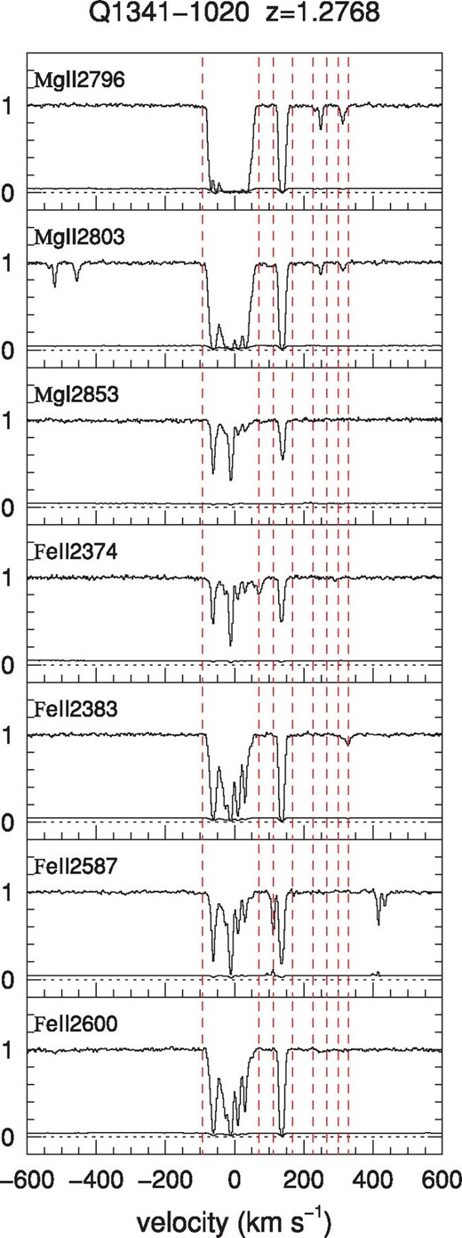
VLT/UVES profiles of Mg ii λ2796, Mg ii λ2803, Mg i λ2853, Fe ii λ2374, Fe ii λ2383, Fe ii λ2587 and Fe ii λ2600 (if covered) for the strong Mg ii absorption lines systems in our sample. The spectra are normalized and the different transitions are aligned in velocity space (zero-point corresponds to the optical depth mean of the Mg ii λ2796 profile). The vertical dashed lines delimit the regions in which Mg ii λ2796 is detected. (This is a sample of the complete figure; see the Supporting Information with the online version of the article for Figs 1.2–1.87.)

Open in new tabDownload slide

Open in new tabDownload slide

Open in new tabDownload slide

Table 1

Rest-frame equivalent widths for target transitions

Table 1 lists the rest-frame equivalent widths or equivalent width limits for the Mg ii, Fe ii and Mg i transitions of the 87 strong systems. Among them, 58 systems are moderately strong ( Å) and 29 systems are very strong absorbers ( Å). Blanks in Table 1 represent cases where the wavelength of the relevant transition was not covered in the VLT/UVES spectrum. In cases where the Fe ii transition or Mg i was covered, but not detected, 3σ upper limits are given. We visually inspected every Fe ii absorption feature, and carefully compared their profiles to each other and to the Mg ii profiles, in order to confirm that they were consistent. We rejected deviant parts of these components, mostly caused by blends with different transitions from systems at other redshifts. In cases where blends prevented the measurement of an accurate equivalent width, we place lower limits by avoiding the blended region and upper limits by including it. These results appear as a range of values in Table 1 (e.g. 0.354–0.426 Å for the W_r(2587) measurement for the absorption system at z_abs = 1.672 in the spectrum of Q0237−0023). When systems suffered from severe blending such that the above-mentioned procedure was not possible, we just include W_r upper limits. Fe ii λ2383 and Fe ii λ2600 are the strongest of the Fe ii transitions, and thus when Mg ii is saturated they may also be saturated. Therefore, we measured other weaker Fe ii transitions (Fe ii λ2374 and Fe ii λ2587), that are less likely to be saturated, and thus provide more leverage on an accurate measurement of the Fe ii.

In Figs Fig. 2–4 we characterize the Mg ii absorption properties of our sample. Fig. 2 shows the cumulative equivalent width distribution of Mg ii λ2796 for our sample of strong Mg ii absorbers. Fig. 3 shows the binned rest-frame Mg ii λ2796 equivalent width distribution. The distribution of equivalent widths is similar to that for the unbiased survey of Nestor et al. (2005), however, our sample has a slightly larger number of moderately strong systems relative to very strong systems. This small difference does not represent a problem for the present study, since our aim is to compare the same types of systems at different redshifts.

Figure 2

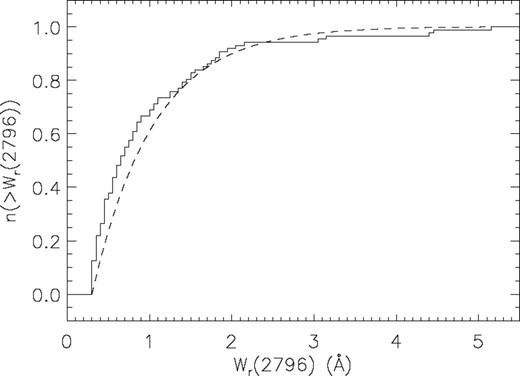
Cumulative Mg ii λ2796 equivalent width distribution for the systems detected in this study (shown as a solid line). Dashed line represents the distribution of systems in the larger sample of Nestor et al. (2005) using the median of our sample (〈z〉 = 1.268).

Open in new tabDownload slide

Figure 3

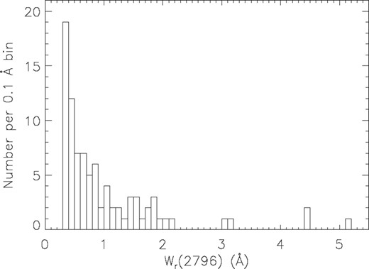
Distribution of the rest-frame equivalent width (W_r) of Mg ii λ2796 for the systems detected in this study. Most of the systems found lie in the lower part of the W_r range. The very strong systems comprise ∼33 per cent (29/87) of the total sample. Only ∼8 per cent (7/87) of all systems present W_r ≥ 2 Å.

Open in new tabDownload slide

Figure 4

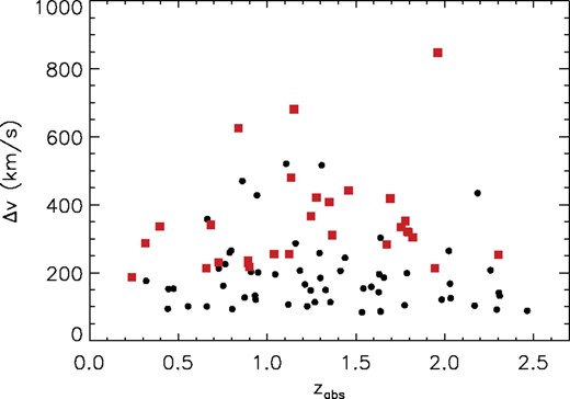
Redshift distribution of the strong Mg ii λ2796 in this study. The top panel shows rest-frame equivalent width of Mg ii versus the absorption redshift. Black circles represent the moderately strong absorption systems (0.3 <W_r < 1.0 Å) and red squares are used for very strong systems (W_r > 1.0 Å). Errors in W_r are smaller than the symbol sizes. The bottom panel shows a histogram of the redshift distribution. The total histogram represents the distribution of all systems (all symbols in top panel), and the red area the distribution of very strong systems with Å (red squares in top panel).

Open in new tabDownload slide

Fig. 4 presents the distribution of the Mg ii absorption systems in equivalent width–redshift (W_r–z_abs) parameter space. The top panel shows versus redshift for the 87 strong Mg ii absorption systems in our study. Throughout this paper we display moderately strong Mg ii absorption systems (0.3 < W_r < 1.0 Å) as black circles and very strong Mg ii systems (W_r > 1.0 Å) as red squares. The bottom panel shows the binned absorption redshift (z_abs) distribution of all the systems in top panel (in white). The 87 systems are roughly uniformly distributed over the absorption redshift range, from z_abs = 0.238 to 2.464, with their mean at 〈z〉 = 1.297. The redshift histogram for only the very strong Mg ii systems (red/shaded) is superimposed. The distributions in redshift for moderately strong (〈z〉 = 1.322) and very strong systems (〈z〉 = 1.247) are not different at a statistically significant level [the Kolmogorov–Smirnov (K–S) tests show that they are drawn from the same distribution]. However, we note that there is only one very strong system with z > 2.

3 Results

As mentioned in Section 1, the Fe/Mg abundance ratio is a tracer of the star formation history of a galaxy. For typical physical properties of interstellar gas, most of the Mg and Fe are in the form of Mg ii and Fe ii, respectively. Thus, although we detected Mg i (Fe i is almost never present, however, see Jones et al. 2010), hereafter we will focus on Mg ii and Fe ii. For some of the strong absorbers in this study, and more likely for the very strong absorbers, Fe ii λ2383 and Fe ii λ2600 are saturated, as well as Mg ii (see Fig. 1). Thus for these Fe ii transitions, there is a slower W_r(Fe II) increase, with increasing Fe ii column density, reducing the leverage of the W_r(Fe II)/W_r(Mg II) ratio in determining evolutionary trends. We compensate for this by using weaker Fe ii transitions, such as λ2374 and λ2587, which are less saturated, and for many systems do not show evidence of saturation. Since Fe ii λ2587 is more often covered in this VLT/UVES sample, we often emphasize it in drawing conclusions.

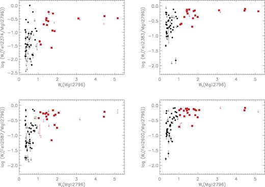
Fig. 5 shows the distribution of ratios of W_r(Fe II)/W_r(Mg II) with respect to W_r(Mg II) for the four Fe ii transitions measured in this study: Fe ii λ2374, Fe ii λ2383, Fe ii λ2587 and Fe ii λ2600. The ratio of W_r(Fe II)/W_r(Mg II) approaches unity as increases, since both the Fe ii and the Mg ii are saturated for the strongest systems. Fe ii λ2374 and Fe ii λ2587 show the largest range of ratio values for the very strong absorbers since they are less saturated than the other two Fe ii transitions. Although our number statistics are small for values of Å, all of our data points in that range have large ratios, fairly close to 1, even for Fe ii λ2374 and Fe ii λ2587.

Figure 5

Ratio of to , for the four Fe ii transitions measured in this study, versus equivalent width of the blue member of the Mg ii doublet (). Black circles represent moderately strong Mg ii absorption (0.3 < W_r < 1.0 Å) and red squares very strong Mg ii absorption (W_r > 1.0 Å). Arrows indicate upper limits (for blends in Fe ii as well as for cases with no detection), and error bars with no central symbol indicate cases where we estimated an upper and lower limit value for the Fe ii measurement (see ). The number of data points is not the same among the four panels due to the non-uniform coverage of the Fe ii transitions in the VLT/UVES spectra. As the values of increase, values tend to increase as well, and when both profiles show signs of saturation, the ratio W_r/ approaches unity. The figure shows how Fe ii λ2374 and Fe ii λ2587 display a larger range of W_r/ values than Fe ii λ2383 and Fe ii λ2600, because the former two transitions are weaker than the latter.

Open in new tabDownload slide

Section Fig. 6 shows the distribution of ratios of W_r(Fe II)/W_r(Mg II) in absorption redshift (z_abs), again for the four Fe ii ions measured in this study. We can see that these distributions for the two different absorption classes (moderately strong and very strong) show different trends. While moderately strong Mg ii absorption systems (black circles) present a wide range of W_r(Fe II)/W_r(Mg II) ratios, independent of redshift, very strong (red squares) Mg ii absorbers are preferentially present in certain regions of the W_r–z_abs parameter space. For very strong Mg ii absorbers (red symbols) at lower redshifts (z_abs < 1.2 in our sample, see below) W_r(Fe II)/W_r(Mg II) is concentrated at higher values, and there are few absorption systems with small ratios of W_r(Fe II)/W_r(Mg II). As redshift increases, a wider range of the ratio is found. As we showed in Fig. 4, there are a sufficient number of very strong systems at low redshift (as compared to high redshift) that we can be confident that this trend is not due to small number statistics.

Figure 6

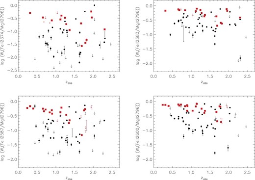
Ratio of versus absorption redshift (z_abs) for the four Fe ii transitions studied. Symbols are equivalent to those in Fig. ⁵. The distribution of moderately strong Mg ii absorbers seems to cover a large range of at all redshifts. In contrast, very strong Mg ii absorbers at lower redshifts (z_abs < 1.2) appear to cluster at high values of , which they do not do at higher redshifts.

Open in new tabDownload slide

The difference in the distribution of W_r(Fe II)/W_r(Mg II) between low and high redshift, for very strong absorbers, is clear from visual inspection of Fig. 6: at low redshift, the very strong Mg ii absorbers show near-unity W_r ratios while there is a much larger spread at high redshift, extending to smaller W_r ratio values. We proceed to quantify the significance of this trend by using several statistical techniques (Table 2). We investigate the probability that two subsamples were derived from the same population by performing K–S and Anderson–Darling (A–D) tests. The A–D test is a modification of the K–S test and gives more weight to differences in the tails of the distribution of the data (Scholz & Stephens 1987). Table 2 includes the comparisons between the W_r ratio distributions of moderately strong and very strong systems, and between high- and low-redshift subsamples of each. To divide each sample into low- and high-redshift subsamples we compute the median of the z_abs values, excluding upper limits, for each Fe ii transition and average them, which yields 〈z_abs〉 = 1.20.

Table 2

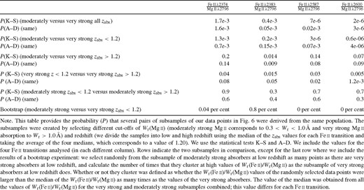
Statistical results on very strong and moderately strong absorption systems

Open in new tabDownload slide

The results in Table 2 confirm that the W_r(Fe II)/W_r(Mg II) distribution for moderately strong absorption systems is not consistent with that for the very strong absorption system population. We see that this difference is more significant in the low-redshift bin (see second row of Table 2) with W_r(Fe II)/W_r(Mg II) approaching unity for the very strong systems (see Fig. 6). Through bootstrapping, we found that in only ≤0.8 per cent of the realizations of the moderately strong sample at low redshift were there as many large W_r(Fe II)/W_r(Mg II) values (larger than the median of W_r(Fe II)/W_r(Mg II)) as in the very strong sample at low redshift (see Table 2 for more details). At higher redshifts, there is still some difference between the W_r(Fe II)/W_r(Mg II) values for very strong and moderately strong samples (see third row of Table 2), but it is not as pronounced.

A comparison of the low- and high-redshift subsamples of very strong absorption systems shows that there is only a small probability that they share the same parent population (see fourth row of Table 2). The largest probability of of the low- and high-redshift subsamples coming from the same parent population is for Fe ii λ2374, . Moderately strong absorption systems show no such difference (see fifth row of Table 2). Thus we conclude that there is a significant evolution in redshift in the W_r(Fe II)/W_r(Mg II) distribution for very strong Mg ii absorbers, but not for moderately strong absorbers.

The left-bottom quadrant of each of the Fig. 6 panels is almost, but not completely, devoid of very strong systems (red squares), thus we would like to comment on the exceptions that do lie in this quadrant. Furthermore, there are a few upper limits on the Fe ii measurements of each transition (red arrows), due to significant contamination, and some of these values could, in principle, come down into this quadrant if they could be accurately measured. In the case of the system at z_abs = 0.8919 towards Q0300+0048 the spectrum is very noisy (S/N < 5; see Fig. 1) around the Fe ii λ2374, Fe ii λ2383 and Fe ii λ2587 transitions, so a point does not appear on those panels. However, the quality of the spectrum at the position of Fe ii λ2600 is higher, and it does appear to yield a relatively low value of W_r(Fe II)/W_r(Mg II), which is apparent in the bottom right-hand panel of Fig. 6. A different situation applies in the case of the z_abs = 1.0387 system towards CTQ 0298, another of the low-redshift data points with a low value in the bottom right-hand panel. The Fe ii absorption for the transitions shortward of 2600 Å lie in the Lyα forest of CTQ 0298, and the resulting blends only allow us to place upper limits on for those transitions. In the case of the z_abs = 0.7261 system towards Q0453−0423, Fe ii λ2374 and Fe ii λ2383 appear to be also blended with other ions, but it is likely that their actual W_r values are close to the upper limits, which implies that their W_r(Fe II)/W_r(Mg II) values are truly in the upper-left quadrant. We have good estimates for the unblended Fe ii λ2587 and Fe ii λ2600 measurements which show large values of the W_r(Fe II)/W_r(Mg II). Finally, all of the Fe ii transitions associated with the z_abs = 1.1335 system towards Q1621−0042 suffer from severe blending in the Lyα forest, thus it is impossible to determine the true W_r values. Having considered these points, we conclude that, with a few possible exceptions, there is a true deficit of small W_r(Fe II)/W_r(Mg II) values for very strong Mg ii absorbers at low redshift.

3.1 Mg ii profile evolution

Fig. 6 shows there is an evolution of the W_r(Fe II)/W_r(Mg II) ratio of very strong Mg ii absorbers. We investigate the profile shape evolution of Mg ii for these systems in order to consider how it might affect the W_r(Fe II)/W_r(Mg II) ratio.

Fig. 7 includes all the normalized profiles of very strong Mg ii systems in our sample, and their corresponding Fe ii λ2587, ordered by increasing z_abs. In cases where Fe ii λ2587 is not covered, another transition is used as indicated on the panels in the figure. We find that the profile shape of Mg ii varies from a predominance of ‘boxy’ profiles at low redshift to the inclusion of more kinematically extended and less saturated Mg ii profiles at high redshift, as would be expected for outflows/superwinds.

Figure 7

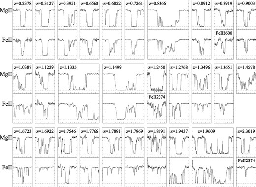
Normalized Mg ii and Fe ii profiles of the very strong Mg ii systems in our sample, in increasing order of z_abs, which is indicated at the top of each spectrum. Mg ii λ2796 and Fe ii λ2587 are plotted unless otherwise noted. There is no spectral coverage of Fe ii in the spectrum of Q1418−064 for the absorber at z_abs = 1.4578. Velocity ranges are (−250, 250) km s⁻¹ in the single boxes and (−500, 500) km s⁻¹ in the double boxes, thus the velocity scale is the same in all boxes, except for the case of Q0551−3637 at z_abs = 1.9609, where the range is (−600, 400) in order to include the entire profile. Dotted horizontal lines indicate flux zero.

Open in new tabDownload slide

Fig. 8 places the very strong Mg ii and Fe ii λ2587 absorption profiles at their corresponding points of the parameter space. This allows us to examine the relationship between profile shape and the W_r(Fe II)/W_r(Mg II) ratio. We can see from Fig. 8 that the evolution in the Mg ii profile kinematics with redshift seen in Fig. 7 is related to the evolution seen in Fig. 6 of the values of W_r(Fe II)/W_r(Mg II) of the very strong Mg ii systems. Most of the kinematically complex, broad profiles correspond to small W_r(Fe II)/W_r(Mg II) ratios at high redshift. We discuss this effect in Section 4.1 and, in Section 4.2, contrast it with the previous analysis of W_r(Fe II)/W_r(Mg II) for weak Mg ii systems.

Figure 8

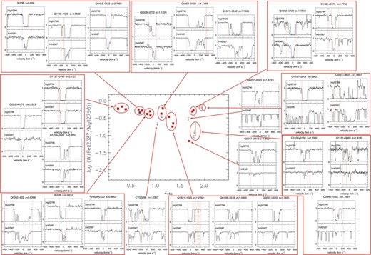
Mg ii λ2796 and Fe ii λ2587 profiles of very strong Mg ii systems (W_r > 1.0 Å) in the parameter space of versus z, which was previously displayed in Fig. ⁶ (symbols are equivalent). For ease of location, we have grouped contiguous systems in boxes and circles. The figure shows that while ‘boxy’ profiles appear at both low and high redshift, they are more predominant at low redshift. On the other hand, systems with ‘outflow/superwind’ type profiles (less saturated and showing larger velocity spreads) are only present at high redshift, and correspond to the systems with smaller values of .

Open in new tabDownload slide

3.2 Kinematical properties

To quantify the evolution we describe in Section 3.1, we also perform kinematic analysis on the Mg ii profiles of the systems in our sample. We saw in Figs ⁷ and ⁸ that systems with larger kinematically spreads tend to be more predominant at higher redshifts. We quantify this effect by calculating the velocity spread, which is a measure of the full absorption line width (in units of velocity), defined as

where v_low and v_high correspond to the minimum and maximum velocity of the absorption, defined by a 3σ absorption detection. Fig. 9 shows the velocity spreads (Δv) of the Mg ii λ2796 profiles in our sample. The distribution of Δv for moderately strong systems (black circles) is similar at all redshifts, but we find differences between the very strong absorbers (red squares) at low and high redshift. The median of the low- and high-redshift values of Δv differs (255 and 334 km s⁻¹, respectively) and the K–S test shows there is a probability of only 0.03 that both subsamples derive from the same population. If we omit the outliers of Δv > 600 km s⁻¹, the K–S test shows the two distributions to be different at an even larger significance level ().

Figure 9

Velocity spread versus absorption redshift of the 87 systems analysed. Symbols are equivalent to those in Fig. ⁵. Strong Mg ii absorption profiles (black circles) show a homogeneous distribution with redshift, but very strong Mg ii absorption profiles (red squares) show a significant difference in their median value of velocity spread between low (z_abs < 1.2) and high (z_abs > 1.2) redshift.

Open in new tabDownload slide

Fig. 10 shows the absorbed pixel fraction (APF) distribution of the Mg ii λ2796 absorption profiles, as a function of redshift. The APF is defined as the fraction of pixels with detected absorption over the entire velocity spread of the profile (Δv), as used in Mshar et al. (2007). The APF equals one in profiles where there is absorption over the entire velocity range, and it helps to quantify the separation between components in the absorption profile whenever the values are smaller. In Fig. 10 it can be seen that there is a large concentration of values with continuous coverage (APF equal 1). The majority (70 per cent; 61/87) of the absorbers in our sample show a complete absorbed coverage range, and 80 per cent (70/87) show a complete or close to complete (APF >0.95) coverage. We obtain slightly larger percentages if we restrict our computations to the very strong absorbers alone (72 and 86 per cent, respectively).

Figure 10

Absorbed pixel fraction versus absorption redshift of the systems in our sample. Values of 1 indicate systems where the whole velocity range is absorbed. Symbols are equivalent to those in Fig. 5.

Open in new tabDownload slide

As in Mshar et al. (2007), we find differences between the low- and high-redshift systems. High-redshift systems tend to show APF values closer to 1, which indicates that the absorption cover the full velocity range, while at low redshift it is more likely to find APF values lower than 1. This is due to a tendency for the high-redshift systems to have weak components connecting the stronger absorbing regions.

Because in the case of very strong absorbers, so many APF values are close to unity, this measurement does not provide much leverage in determining kinematic evolution. To further quantify the shape of the profiles, and in particular how ‘boxy’ or spread out they are, we define their dimensionless average depth as the fraction of normalized flux that is absorbed, averaged over the full range of Δv. In the case of a completely rectangular absorber, the depth would be equal to one (since our W_r is defined from normalized spectra). This averaged depth is equivalent to the D-index as defined in Ellison (2006), and posteriorly reviewed in Ellison, Murphy & Dessauges-Zavadsky (2009), except that we include the whole velocity range (Δv) in the average. We present this depth measurement versus some other properties of our sample in Figs 11–13. Figs Figs 11 and Figs 12 show profile depths versus W_r(Mg ii) and Δv, respectively. There is an envelope at the lower end of the depth distribution which depends on the value. This is regulated by the typical maximum Δv value for the profiles. In other words, we do not find shallow profiles with large values (see Figs ⁷ and ⁸), which would result from very large Δv values and would lead to a departure from the –Δv correlation. Only the several profiles with the largest have Δv ≳ 500–600 km s⁻¹. Thus, a given equivalent width can only result from a depth larger than some minimum value. Completely ‘boxy’ profiles are also rare, since weaker subsystems are common; because of this and the gradual recovery of profiles to meet the continuum, there is also a natural high limit for the depth value. Fig. 12 shows that moderately strong and very strong Mg ii absorbers occupy a different region of the depth–Δv parameter space. This is also partly due to the correspondence between larger W_r and larger Δv. Once saturation is present the only way to increase the W_r is through increasing the Δv of the profile.

Figure 11

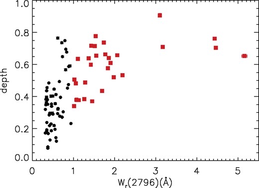
Profiles' depth distribution with rest-frame equivalent width of Mg ii λ2796. Depth is defined as the fraction of flux absorbed, averaged over the velocity width of a profile. Symbols are equivalent to those in Fig. 5. Moderately strong Mg ii absorption profiles (black circles) show a larger range of depths than very strong Mg ii systems (red squares), which show a minimum depth of ∼0.3. This is not surprising because there is a correlation between and Δv.

Open in new tabDownload slide

Figure 12

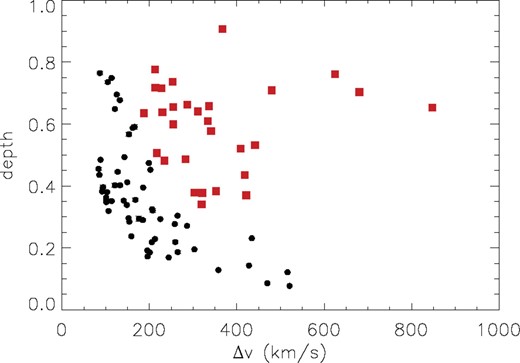
Depth versus Δv of the profiles in our sample. Symbols are equivalent to those in Fig. 5. Moderately strong (black circles) and very strong (red squares) Mg ii absorbers are confined in different regions of the depth–Δv parameter space.

Open in new tabDownload slide

Figure 13

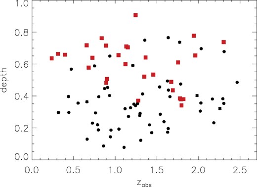
Depth versus absorption redshift of the profiles in our sample. Symbols are equivalent to those in Fig. 5. We can see that while the moderately strong Mg ii absorption profiles (black circles) show a similar distribution at low and high redshift, very strong ones (red squares) show evolution with a larger range of depths at high redshifts than at low redshifts.

Open in new tabDownload slide

Fig. 13 shows the distribution of depth with absorption redshift. There is a clear evolution for the very strong Mg ii absorption profiles, which is not present for the moderately strong ones. An A–D test results in a probability of only P = 0.03 that the depths of the low-redshift subsample of very strong absorbers are drawn from the same population as those of the high-redshift subsample. The distribution of depths of the moderately strong (black circles) and very strong absorbers (red squares) at low redshift is significantly more different (P(K–S) = 4e-7) than the distribution of the two subsamples at high redshift (). Because the depth is influenced both by W_r(Mg ii) and Δv, evolution of W_r(Mg ii) would play a role into depth evolution. However, in Fig. 4 we already showed that there is no significant evolution of W_r(Mg ii) with redshift in our sample, thus changes in Δv must dominate. Another way to consider the trend of depth evolution in Fig. 13 is to note that the cluster of very strong absorbers with depth values ∼0.4 in Fig. 12 are all in our high-redshift sample. The presence of small depths at high redshift, but not at low redshift, is reminiscent of the evolution of shown in Fig. 6, and we will consider this connection in Section 4.

4 Summary and Discussion

In a large sample (81) of high-resolution VLT/UVES spectra, we have found 58 moderately strong (0.3 < W_r < 1 Å) and 29 very strong (W_r > 1 Å) Mg ii absorption systems, and searched for accompanying Fe ii and Mg i absorption. We have investigated the profile shape evolution of Mg ii as well as the evolution of the ratio. Here we summarize the main results of this study.

• For moderately strong Mg ii absorbers, the ratio W_r(Fe II)/W_r(Mg II, does not evolve significantly from z ∼ 2.5 to ∼0.2.

• In contrast, very strong Mg ii absorbers show evolution in W_r(Fe II)/W_r(Mg II, with a deficit of small values at low redshift.

• Moderately strong Mg ii absorber profiles do not evolve significantly from z ∼ 2.5 to ∼0.2, as quantified by profile velocity spread and depth.

• However, very strong Mg ii absorbers at low redshift all have relatively high profile depth values, while those at high redshift have a wider range of values (more similar to the range for moderately strong systems).

4.1 Possible causes for the evolution of very strong Mg ii absorbers

It is not surprising to find an evolution in the population of very strong Mg ii systems. Nestor et al. (2005) already showed an excess of these systems at high redshift, relative to absorbers with smaller equivalent widths. Among the very strong Mg ii absorber population, the deviations from cosmological evolution are larger as increases (Nestor et al. 2005).

Given the observed evolution in the ratio for the class of very strong Mg ii absorbers, shown in Fig. 8, we consider several plausible reasons. These include (1) a changing ionization rate due to evolution of the extragalactic background; (2) a change in the level of α-enhancement due to changing contributions of Type II and Type Ia SNe to the absorbing gas; (3) a change in the kinematics of the profiles, including different levels of saturation and velocity spreads which affect the equivalent widths of Fe ii and Mg ii differently. Here we will consider the expected effect of each of these factors.

The parameter space of very strong Mg ii absorbers shows large W_r(Fe II)/W_r(Mg II at both low and high redshift, but small only at high redshift (see Figs ⁶ and ⁸). The profiles of very strong Mg ii absorbers (those with W_r >1 Å) are almost always saturated in Mg ii, and sometimes saturated even in the weakest accessible Fe ii transition as well (see Fig. 7). We should first consider this when interpreting the observed absence of low W_r(Fe II)/W_r(Mg II values in this population at low redshift. As shown in Section 3.1, Fig. 8 indicates that there is an evolution in the Mg ii profile kinematics that is relevant for our interpretation of the W_r(Fe ii)/ evolution for very strong Mg ii absorbers. At low redshift, many of the systems show ‘boxy’ profiles and they tend to have fewer, if any, satellite clouds around their compact, ‘boxy’ portions. Therefore, they do not have a significant range of velocity that is unaffected by saturation in Mg ii. A typical example of these ‘boxy’ profiles is the z = 0.2378 system towards Q0952+0179, shown in Fig. 1 (also see Figs ⁷ and ⁸). Because the weaker Fe ii λ2374 and Fe ii λ2587 transitions are not strongly saturated for many components, the Fe ii equivalent widths are less affected by saturation effects.

Furthermore, it is important to note that we are only comparing the equivalent widths of the Mg ii and Fe ii transitions, and not their column densities. In the case of a saturated profile, of course it is not possible to measure the column density, and we should interpret the equivalent width as a lower limit on how much material is present. For the W_r(Fe II)/W_r(Mg II ratio, in cases where the Mg ii is saturated and the Fe ii is not, our values are therefore upper limits. This alone could lead to the absence of very strong Mg ii absorbers with small W_r(Fe II)/W_r(Mg II values. The question then is why very strong Mg ii absorbers at high redshift do often have small values of W_r(Fe II)/W_r(Mg II, while those at low z do not.

The answer can be seen by examining the Mg ii profile shapes of the high-redshift systems in the lower right-hand quadrants of Figs ⁶ and ⁸. These profiles show components more spread out in velocity space, with several subsystems within the absorption profile. Because of this kinematic spread, even if the column densities and numbers of components are the same as for the low-redshift systems, we will see less saturation. This is evident in the existence of some low values of profile depth (see Fig. 13) among the high redshift very strong Mg ii absorbers. Several ‘boxy’ saturated Mg ii profiles are apparent among the high-z systems as well, and these have large values of W_r(Fe II)/W_r(Mg II, as did all of the systems at lower redshift. If the Mg ii profile suffers from significant saturation, the W_r(Fe II)/W_r(Mg II value is an overestimate and it is impossible for it to be small. In order that a very strong Mg ii absorber not have significant saturation it must be kinematically spread, and such kinematics are apparently more common at high redshift than at low redshift.

This is consistent with the conclusions of Mshar et al. (2007) on the evolving kinematics of a smaller sample of very strong Mg ii absorbers. That study found that complex systems with many components spread in velocity are more common at high redshift than at low redshift. For example, profiles typically associated with superwinds (Bond et al. 2001; Ellison et al. 2003) show large velocity spreads. The excess of very strong Mg ii absorbers at high redshift, found in Nestor et al. (2005), may be related to our findings if the excess systems correspond to outflows/superwinds, and are thus evolving together with the SFR in galaxies.

Returning to the three effects that could affect evolution of the W_r(Fe II)/W_r(Mg II ratio in very strong Mg ii systems, we have found that kinematic evolution of this population could explain the observed trend. This does not necessarily mean that ionization and abundance pattern changes are not taking place as well, just that we are not able to get an indication of the ionization parameter or abundance pattern for the saturated systems. In other words, some of the systems with ‘boxy’ profiles in Mg ii both at high and low redshift could have higher/lower ionization parameters or could be α-enhanced/depleted relative to the others, but would still not have small W_r(Fe II)/W_r(Mg II ratios relative to others because of saturation of the Mg ii. At higher redshift, however, it seems likely that systems with large kinematic spread and small values of W_r(Fe II)/W_r(Mg II (bottom right-hand quadrant of Fig. 8) are different than the ‘boxy’ profiles systems (top right-hand quadrant of Fig. 8) that also appeared in this redshift range. The strong Mg ii absorbers, with Å, also have the full range of W_r(Fe II)/W_r(Mg II, but not all of them with large values are strongly saturated in Mg ii.

It is natural to expect an absorber population to be more ionized at higher redshift because of the evolution of the extragalactic background radiation. This is due both to the changes in the ionizing extragalactic background radiation and due to the more intense local radiation field in starbursts, both of which are a consequence of the higher global SFR at higher redshift. Even without a contribution from local star formation, the photon number density, log n_γ changes from −4.7 cm⁻³ at z = 2 to −5.7 cm⁻³ at z = 0.3, which will lead to a significant difference in the ionization parameter affecting our Mg ii absorbing clouds. In particular, is relatively constant for ionization parameter log U < −4.5 but decreases rapidly from log U = −4 up to higher values. At z = 2, a cloud with n_H = 0.1 cm⁻³ would have log U = −3.7, while it would have log U = −4.7 at z = 0. If instead the Mg ii cloud has lower densities, for example n_H = 0.01 cm⁻³, it would result in log U = −2.7 at z = 2, and log U = −3.7 at z = 0. While the difference of between low- and high-redshift systems would be barely noticeable in the case of n_H = 0.1 cm⁻³, clouds of densities of n_H = 0.01 cm⁻³ would have significantly lower at high redshift than at low redshift. Thus, the systems with small values would result from systematically lower density clouds. A larger range of densities (and thus log U) would lead to ionization of the Fe ii and would give rise to small at high redshift, and thus we would expect more systems with small at high redshift. Although this clearly matches the observed behaviour for very strong Mg ii absorbers, we cannot measure this effect since it is disguised by the saturated Mg ii profiles in many of the systems.

Similarly, α-enhanced systems are expected to be more common at higher redshift, where the SFR is higher. It takes time for a stellar population to produce Type Ia SNe, leading to about a 1 billion year delay before the iron abundance would be elevated to the solar value, relative to magnesium. As will be discussed further in , Narayanan et al. (Section 2007) noted that this delay could be a significant contributing factor to the absence of weak Mg ii absorbers with large W_r(Fe II)/W_r(Mg II. The larger kinematic spreads of some of the high redshift very strong Mg ii absorbers may be related to enhanced star formation/starburst and wind activity at high redshift. Thus, these systems would be expected to be the α-enhanced systems with small W_r(Fe II)/W_r(Mg II values. It is plausible that there would be fewer such α-enhanced systems at low redshift. Furthermore, a stronger depletion of Fe relative to Mg would result in a smaller W_r(Fe II)/W_r(Mg II. It is known that Mg returns to the gas phase faster than Fe (Fitzpatrick 1996). Indeed, mild and high Fe depletion has been previously observed in some DLA and sub-DLA systems, both at low and high redshift (e.g. Ledoux, Bergeron & Petitjean 2002; Meiring et al. 2008, 2011; Noterdaeme et al. 2010). Like ionization effects, both α-enhancement and depletion of Fe contribute in the right direction to lead to a relative absence of very strong Mg absorption in the lower right-hand quadrant in the W_r(Fe II)/W_r(Mg II versus z diagram. However, we cannot tell if the lower left-hand quadrant is vacant because of the lack of α-enhancement/greater depletion of Fe at low redshift, or just because low-redshift systems preferentially have kinematics that lead to saturation of Mg ii and Fe ii.

We conclude that, in the case of very strong Mg ii absorbers, low values of W_r(Fe II)/W_r(Mg II at high redshift could be due to a larger ionizing radiation field or to α-enhancement of a larger fraction of systems, but the effects cannot be quantified in these mostly saturated systems. We also cannot be certain of the cause of the absence of low W_r(Fe II)/W_r(Mg II values at low redshift, because all the low-redshift systems in our sample have significant saturation of Mg ii and Fe ii. The significant evolution that we have detected, therefore, is the evolution of the kinematics of the Mg ii profiles, from a mixture of saturated, flat bottom profiles and kinematically spread components at high redshift to only predominantly saturated, flat bottom profiles at low redshift.

This is quite consistent with several recent studies of the nature of DLAs and sub-DLAs, which are coincident with the population of very strong Mg ii absorbers. Since very strong Mg ii absorbers are selected by an equivalent width criterion, they are not necessarily all among the highest column density absorbers, and thus are not all DLAs. The equivalent width of Mg ii can be very large either because the total column density of material is very large (thus it would likely be a DLA), or because the kinematic spread of components is large enough that the equivalent widths add up to a large total (in which case the system might be a DLA, but may also be a sub-DLA or even a Lyman limit system).

Indeed, the populations of DLAs and sub-DLAs have important intrinsic differences. Kulkarni et al. (2010) show that DLAs have systematically lower metallicities than sub-DLAs (based on Zn measurements), and furthermore that they have a smaller velocity spread than sub-DLAs. Kulkarni et al. (2010) suggest that the differences in metallicities between DLAs and sub-DLAs could be due to different star formation histories, where the galaxies observed as sub-DLAs undergo more rapid star formation. Both Kulkarni et al. (2010) and Nestor et al. (2011) suggest that DLAs are often dense regions in ordinary galaxies, while sub-DLAs are of higher metallicity and extended kinematics such as one would expect from a superwind. All these results would be consistent with the boxy profiles that we see in Mg ii tending to be DLAs, while the kinematically spread systems that are more common at higher redshift, would tend to be sub-DLAs, where the star formation is more likely to happen. Then, our finding that small W_r(Fe II)/W_r(Mg II values for very strong Mg ii absorbers are only present at high redshifts could be due to both α-enhancement and kinematics, expected from outflows/superwinds.

Another related factor that would condition the shape of the Mg ii profiles may be the association of the subset of very strong absorbers with galaxy overdensity regions such as groups or clusters where interactions and mergers are common. Nestor et al. (2007) found that field imaging of a subset of the strongest Mg ii absorbers ( Å) at low redshift (0.42 < z < 0.84) indicates that pairs of galaxies, often with distorted morphologies, and starburst related phenomena, are coincident with these Mg ii systems. Although, this redshift range is lower compared to the high z very strong systems in our sample, interactions would be only more frequent at high redshift. If these very strong Mg ii absorption systems are selecting group environments, star formation is also going to be higher compared to the average for that redshift (e.g. Kennicutt et al. 1987; and more recently Wong et al. 2011), which would push this subset of absorbing gas in the direction towards lower W_r(Fe II)/W_r(Mg II ratios. We find that our results are consistent with this scenario. In our sample, for one of the strongest Mg ii systems (Q0002−422, z = 0.837), Yanny, York & Williams (1990) have identified several emission line sources within 100 kpc, which indicates that there is probably a group environment (also see York et al. 1991). Similarly, the very strong Mg ii system in the line of sight of Q0453−423 at z = 0.726 also has multiple galaxies associated with it (Yanny et al. 1990).

4.2 Comparison to the evolution of weak Mg ii absorbers

The evolution of weak systems and their ratio was presented in Narayanan et al. (2007, 2008). Fig. 14 shows the evolution of the W_r ratio for very strong Mg ii absorption systems (red squares, top) and the weak Mg ii systems (green triangles, bottom) from Narayanan et al. (2007). For very strong absorption (top) is measured in the Fe ii λ2587 transition because it is weak enough not to be saturated, but is the most often observed Fe ii transition in our sample. Weak Mg ii absorption is accompanied by even weaker Fe ii troughs, and since Fe ii λ2383 is the strongest transition, it is the mostly likely to be detected and the one displayed in Fig. 14.³ Weak absorbers reflect a different trend than very strong absorbers: we find that large values are uncommon at higher redshifts, i.e. weak Mg ii systems show a deficit as well, but in the opposite quadrant of the –z parameter space.

Figure 14

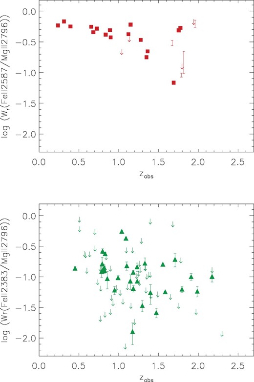
Ratio of versus absorption redshift (z_abs) for the very strong Mg ii systems (top) and weak Mg ii systems (bottom). Symbols are equivalent to those in Fig. ⁵. Two opposite trends are present. There is an absence of very strong absorbers with low ratios at low redshift (top) and an absence of weak absorbers with large ratios at high redshift (bottom). In the case of the very strong absorbers, we chose Fe ii λ2587, because it was less often saturated than the Fe ii λ2383 and λ2600 transitions, and was covered more often than the weaker Fe ii λ2374 transition. For weak Mg ii absorbers, Fe ii λ2383 was chosen because, as the strongest Fe ii transition, it is mostly likely to be detected.

Open in new tabDownload slide

Narayanan et al. (2007) considered the possible causes of the evolution of weak Mg ii absorbers. Since saturation of these weak profiles is fairly rare, the cause of the evolution could be (1) changing ionization or (2) abundance pattern changes in the population of gas clouds that produce these absorbers. In the first case, because of the known evolution of the extragalactic background radiation (higher at higher redshifts) and since Fe ii is more readily ionized than Mg ii, we would need higher density absorbers to populate the large W_r(Fe II)/W_r(Mg II) high-redshift quadrant, than we would at low redshift. In the second case, a delay between the Type II and Type Ia SNe, i.e. an α-enhancement, might help explain the absence of large W_r(Fe II)/W_r(Mg II) values at high redshifts. There may not yet have been time for Type Ia SNe to be active in weak Mg ii absorbing clouds at high redshift, which themselves tend to be less common at z > 1.4 than at lower redshifts (see Lynch, Charlton & Kim 2006; Narayanan et al. 2007, 2008).

In fact, the evolution of the very strong Mg ii absorbers and the weak Mg ii absorbers, though in the opposite sense, may be related. Weak Mg ii absorbers with require an abundance pattern influenced by Type Ia SNe, and their relative absence at z > 1.4 implies that they are related to a population of gas clouds that is not common at high redshifts. As described in Narayanan et al. (2008), this could either be because they are related to dwarf galaxies, in which star formation peaks later, or to a rarity of weak Mg ii clouds because haloes are more crowded so they are more commonly combined to form strong Mg ii absorbers. At least some weak Mg ii absorbers are produced by the same gas clouds that produce the ‘satellite clouds’ of strong Mg ii absorbers, simply viewed from a different vantage point. These are also likely to be analogous to Milky Way high-velocity clouds, at various redshifts (Richter et al. 2009).

What we have seen here is that some fraction of very strong Mg ii absorbers, those that are related to sub-DLAs and to star formation activity, have components spread in velocity space. Their W(Fe II)/W(Mg II) values are consistent with α-enhancement, just as are all of the weak Mg ii absorbers in the same redshift range. Since satellites around very strong Mg ii absorbers are analogues to isolated weak Mg ii absorbers, and since these are common in high redshift sub-DLAs, the picture of α-enhancement in both populations is consistent.

4.3 Conclusions and future work

The main result of this study is the evolution of the population of very strong Mg ii absorbers ( Å) over the redshift range 0.2 < z < 2.5. There is a significant absence of small W_r(Fe II)/W_r(Mg II) values at low redshift, as compared to the full range apparent at high redshift. A major contributing factor to this change is clearly the kinematic evolution of the profiles of the very strong absorbers. At low redshift, Mg ii presents simple, boxy, saturated profiles, while at high redshift there are also Mg ii profiles with multiple components, some unsaturated, that are spread over a larger range of velocity. Thus at high redshift, it is more likely that some of the Fe ii profiles will also be unsaturated, so that small W_r(Fe II)/W_r(Mg II) values can arise.

Other factors could also contribute to the absence of small W_r(Fe II)/W_r(Mg II) values at low redshift. Most notably a small ratio could be indicative of an α-enhanced abundance pattern, which would be characteristic of a young stellar population, such as one contributing to active galactic outflows. The absence of small ratios of Fe ii to Mg ii at low redshift is thus consistent with the idea that outflows are more active at high redshift.

The key to testing the hypothesis that abundance pattern is evolving, in addition to the known evolution in the kinematics, is to determine if the very strong Mg ii absorbers at z > 1.2 that have small W_r(Fe II)/W_r(Mg II) are truly α-enhanced. This requires a separation of saturation effects from the effect of changing abundance patterns. Transitions with lower oscillator strengths should be studied to facilitate this separation. There are numerous Fe ii transitions with various oscillator strengths in the rest frame λ = 1050–2600 Å regime. Since other Mg ii transitions are too weak to be detected, even in these very strong systems, we will need to consider other α-elements for comparison, e.g. Si ii, which has several promising transitions in the rest-frame far-UV, an ionization potential similar to Mg ii, and similar dust abundances at least in the Galactic disc and the interstellar medium (ISM; Cartledge et al. 2006; Whittet 2010). High-resolution quasar spectra with wide wavelength coverage (optical and UV) are thus essential to assessing evolving chemical abundance processes over cosmic time.

Acknowledgments

This research was funded by NASA under grant NAG5-6399 NNG04GE73G, and by the National Science Foundation (NSF) under grant AST-04-07138 and through the REU program. PRH would like to thank those who approached us during talks and posters, because those discussions helped shape the explanations in this paper.

Supporting Information

Additional Supporting Information may be found in the online version of this article:

Figure 1. VLT/UVES profiles.

Please note: Wiley-Blackwell are not responsible for the content or functionality of any supporting materials supplied by the authors. Any queries (other than missing material) should be directed to the corresponding author for the article.

References