


Abstract
The observed abundance of giant arcs produced by galaxy cluster lenses and the measured Einstein radii have presented a source of tension for Λ cold dark matter (ΛCDM), particularly at low redshifts (z ∼ 0.2). Previous cosmological tests for high-redshift clusters (z > 0.5) have suffered from small number statistics in the simulated sample and the implementation of baryonic physics is likely to affect the outcome. We analyse zoomed-in simulations of a fairly large sample of cluster-sized objects, with Mvir > 3 × 10¹⁴ h−1 M⊙, identified at z = 0.25 and 0.5, for a concordance ΛCDM cosmology. These simulations have been carried out by incrementally increasing the physics considered. We start with dark-matter-only simulations and then add gas hydrodynamics, with different treatments of baryonic processes: non-radiative cooling, radiative cooling with star formation and galactic winds powered by supernova explosions, and finally including the effect of active galactic nucleus (AGN) feedback. Our analysis of strong lensing properties is based on the computation of the cross-section for the formation of giant arcs and of the Einstein radii. We find that the addition of gas in non-radiative simulations does not change the strong lensing predictions significantly, but gas cooling and star formation together significantly increase the number of expected giant arcs and the Einstein radii, particularly for lower redshift clusters and lower source redshifts. Further inclusion of AGN feedback reduces the predicted strong lensing efficiencies such that the lensing probability distributions become closer to those obtained for simulations including only dark matter. Our results indicate that the inclusion of baryonic physics in simulations will not solve the arc-statistics problem at low redshifts, when the physical processes included provide a realistic description of cooling in the central regions of galaxy clusters. As outcomes of our analysis, we encourage the adoption of Einstein radii as a robust measure of strong lensing efficiency, and provide the ΛCDM predictions to be used for future comparisons with high-redshift cluster samples.
1 INTRODUCTION
The hierarchical formation paradigm describes a scenario in which small structures form earlier and then merge to form more massive objects. This description within the Λ cold dark matter (ΛCDM) model has been highly successful at explaining observations of structure on a large range of scales and redshifts (e.g. Efstathiou, Sutherland & Maddox ; White & Frenk ; Komatsu et al. ), including the formation of galaxy clusters (e.g. Kravtsov & Borgani ). However, the internal structure of galaxy clusters has posed a challenge. The earliest comparisons between simulated clusters and the observed frequency of gravitational lensing arcs revealed a serious discrepancy between the observations and ΛCDM predictions (Bartelmann et al. ; Li et al. ). More recent comparisons to X-ray-selected clusters find that the discrepancy remains for z < 0.3 and z > 0.5 but results are not definitive due to small simulated sample sizes at higher redshifts and uncertainties with selection procedures and biases (Horesh et al. ; Meneghetti et al. ). In addition, observations of clusters at redshifts 0.1 < z < 0.6 have found higher concentrations and larger Einstein radii than predicted (Broadhurst & Barkana ; Sadeh & Rephaeli ; Zitrin et al. ). These are related problems since both suggest a failure of ΛCDM to correctly infer the distribution of matter in the cores of clusters; the solution may be found in the details of the simulations used to formulate the predictions.
Simulations which only incorporate collisionless particles are commonplace in the literature. Dark matter (DM) structure is evolved under gravity with the effect of baryons ignored. On large scales, the distribution of gas follows the DM potential wells, so the collisionless simulations will suffice; however, on galaxy and group scales, gas cooling, star formation and feedback can alter the gravitational potential significantly (e.g. Blumenthal et al. ; Gnedin et al. ). Early simulations that were used to model the cluster lenses did not incorporate sufficient relevant physical processes (Hattori, Watanabe & Yamashita ; Sadeh & Rephaeli ). These simulations were originally justified by the premise that the temperature of the intracluster medium (ICM) is too hot to allow efficient cooling, so the baryonic matter must simply follow the DM potential and would not have a significant impact on its shape (e.g. Broadhurst & Barkana ). The role of baryons in shaping galaxy clusters has recently become a key point of discussion since hydrodynamic simulations have become more feasible; the findings are that baryons do, in fact, affect the shapes of gravitational potential of the simulated haloes. Gas cooling, for example, leads to adiabatic compression of galaxy haloes preferentially in the cluster centre, allowing more mass to be deposited around the core (Barkana & Loeb ). Cooling and star formation serve to steepen the density profile of clusters and thus increase the mass concentration and the strong lensing cross-section (Lewis et al. ; Gnedin et al. ; Puchwein et al. ; Rozo et al. ; Rudd, Zentner & Kravtsov ; Cui et al. ). Unfortunately, these processes lead to the well-known overcooling problem, in which the cold gas mass and stellar mass in the cluster core are overestimated.
Including in simulations feedback from gas accretion on to supermassive black holes (SMBHs) is a promising solution for overcooling (Sijacki et al. ; Fabjan et al. ; McCarthy et al. ; Teyssier et al. ), while simultaneously reproducing the drop in the cosmic star formation rate (SFR) for z < 2 (e.g. van de Voort et al. ). The resulting feedback from active galactic nuclei (AGN) significantly reduces the gas fraction in simulated galaxy groups and poor clusters (T ≲ 2 keV), but cannot remove gas from the deep potential wells of rich, massive clusters (Puchwein, Sijacki & Springel ; Fabjan et al. ; McCarthy et al. ). While the total baryonic content of massive clusters is relatively unaffected by cooling, star formation and energy feedback, such processes can imply a quite pronounced redistribution of baryons, particularly close to the cluster centre. Duffy et al. () analysed simulated haloes at z = 0 ranging from galaxy to cluster scales. They demonstrated that while radiative cooling increases mass concentration (see also Rudd et al. ), AGN feedback has the opposite effect; clusters modelled with AGN feedback have mass concentrations equal to those modelled with DM only. Consistent with these results, Mead et al. () demonstrated that AGN feedback is able to reduce the strong lensing cross-section for clusters at z = 0.2. Four of the five clusters they simulated had strong lensing efficiencies consistent with their DM counterparts, while the fifth remained a stronger lens.
Many of the previous works investigating the role of baryons in modifying cluster cores have told similar stories: while cooling and star formation either directly or indirectly leads to an increase of mass in the core, and therefore an increase in the strong lensing efficiency, AGN feedback negates this to some extent. Unfortunately, previous studies have had limited samples of massive clusters, especially at high redshift (z ≳ 0.3), and have utilized simulations generated with values for cosmological parameters that have since been revised. The strong lensing studies of Puchwein et al. (), Rozo et al. () and Mead et al. () were undertaken in the 1-year Wilkinson Microwave Anisotropy Probe (WMAP1) type cosmology with σ8 = 0.9. As shown by Macciò, Dutton & van den Bosch (), changing the cosmology from WMAP1 to WMAP3 best-fitting models can lead to a 20 per cent decrease in the predicted mass concentration of relaxed clusters. This is primarily due to the decrease of the power-spectrum normalization, σ8, from 0.9 to 0.7, and the subsequent delay in the assembly of haloes. The current WMAP7 best-fitting values lie between these two extremes; the expected reduction in the concentration of masses considered in this work from WMAP1 to WMAP5/7 is closer to 14 per cent (e.g. Duffy et al. ; Macciò et al. , but see also Prada et al. ).
In this work, we improve upon the aforementioned works by analysing the strong lensing efficiencies of a larger sample of clusters simulated within the currently favoured cosmology (σ8 = 0.8) with only DM, and also including the hydrodynamical treatment of gas, along with cooling, star formation and feedback from both supernova (SN) and AGN. Strong lensing properties of our fairly large sample of massive clusters are analysed at two redshifts, z = 0.25 and 0.5. A description of the cosmological simulations and the cluster sample follows in Section . Earlier studies have characterized strong lensing by the cross-section for the formation of giant arcs. A comparison with observational data requires the cross-section, as a function of source redshift, to be convolved with the source redshift distribution; uncertainties in this source redshift distribution weaken the cosmological test. We, therefore, propose that the Einstein radius is a more robust proxy for strong lensing; critical curves are determined at a single source redshift (usually zs =2), regardless of the range of source redshifts used for lens mass reconstructions. Therefore, in Sections and we present the strong lensing properties for the relaxed subsample and discuss the influence of the baryonic processes; in the former section we characterize strong lensing with the cross-section for the formation of giant arcs, while in the latter we consider the Einstein radii instead. At the end of this section, we describe the strong lensing properties of unrelaxed subsample. These results are then interpreted in terms of variation of the density profiles induced by the presence of baryons in the simulated clusters. Finally, we summarize our findings in Section .
2 SIMULATIONS
2.1 The simulated set of clusters
The set of simulated clusters analysed in this study have been previously presented by Fabjan et al. () and Bonafede et al. (), and a more comprehensive description will be provided in a forthcoming paper (Planelles et al., in preparation), but we describe them in brief here. Cluster haloes have been identified in a low-resolution simulation box having a periodic comoving size of 1 h−1 Gpc for a flat ΛCDM model whose cosmological parameters were chosen as follows: present-day vacuum density parameter ΩΛ, 0 = 0.76, matter density parameter ΩM, 0 = 0.24, baryon density parameter Ωb, 0 = 0.04, Hubble constant h = 0.72, normalization of the matter power spectrum σ8 = 0.8 and primordial power spectrum P(k) ∝ kn with n = 0.96. The parent simulation followed 10243 collisionless particles in the box. Clusters were identified at z = 0 using a standard Friends-of-Friends (FoF) algorithm, and Lagrangian regions around 24 of the clusters found to have masses MFOF > 1015 h−1 M⊙ were resimulated at higher resolution employing the Zoomed Initial Conditions code (zic; Tormen, Bouchet & White ), while resolution is progressively degraded outside these regions, so as to save computational time while still providing a correct description of the large-scale tidal field. The Lagrangian regions were large enough to ensure that only high-resolution particles are present within five virial radii of the central cluster.
Simulations have been carried out using the TreePM smoothed particle hydrodynamics (SPH) gadget-3 code, a newer version of the original gadget-2 code by Springel () that adopted a more efficient domain decomposition to improve the work–load balance. Each resimulation has been repeated with a unique set of included baryonic processes, some of which are analysed here: one simulation set uses collisionless DM particles only; one is a non-radiative run; another two implement a number of processes associated with baryons; one of these two includes AGN feedback. The basic characteristics of these resimulation sets are described below.
DM. Simulations including only DM particles that, in the high-resolution region, have a mass  . The Plummer-equivalent comoving softening length for gravitational force in the high-resolution region is fixed to
  kpc physical at z < 2 while being fixed to
  kpc comoving at higher redshift.
NR. Non-radiative hydrodynamical simulations. Initial conditions for these hydrodynamical simulations are generated starting from those of the DM-only simulations, and splitting each particle in the high-resolution region into one DM and one gas particle, with their masses chosen so as to reproduce the assumed cosmic baryon fraction. The mass of each DM particle is then mDM = 8.47 × 10⁸ h−1 M⊙ and the mass of each gas particle is mgas = 1.53 × 10⁸ h−1 M⊙. For the computation of the hydrodynamical forces, we assume the minimum value attainable by the SPH smoothing length of the B-spline interpolating kernel to be half of the corresponding value of the gravitational softening length. No radiative cooling is involved.
CSF. Hydrodynamical simulations including the effect of cooling, star formation and SN feedback. Radiative cooling rates are computed by following the same procedure presented by Wiersma, Schaye & Smith (). We account for the presence of the cosmic microwave background (CMB) and for the model of ultraviolet/X-ray background radiation from quasars and galaxies, as computed by Haardt & Madau (). Contributions to cooling from each one of the 11 elements (H, He, C, N, O, Ne, Mg, Si, S, Ca, Fe) have been pre-computed using the publicly available cloudy photoionization code (Ferland et al. ) for an optically thin gas in (photo)ionization equilibrium. Gas particles above a given threshold density are treated as multiphase, so as to provide a subresolution description of the interstellar medium, according to the model originally described by Springel & Hernquist (). Within each multiphase gas particle, a cold and a hot phase coexist in pressure equilibrium, with the cold phase providing the reservoir of star formation. We include a detailed description of metal production contributed by SN II, SN Ia and low- and intermediate-mass stars, as described by Tornatore et al. (). Stars of different masses, distributed according to a Chabrier initial mass function (Chabrier ), release metals over the time-scale determined by the corresponding mass-dependent lifetimes (taken from Padovani & Matteucci ). Kinetic feedback contributed by SN II is implemented according to the scheme introduced by Springel & Hernquist (); a multiphase star particle is assigned a probability to be uploaded in galactic outflows, which is proportional to its SFR. For this set of simulations, we assume vw = 500 km s−1 for the wind velocity.
AGN. The same as CSF, with a lower wind velocity of vw = 350 km s−1, also including the effect of AGN feedback. In the model for AGN feedback, released energy results from gas accretion on to SMBHs. This model introduces some modifications with respect to that originally presented by Springel, Di Matteo & Hernquist (, hereafter SMH), to which is largely inspired, and will be described in detail by Dolag et al. (in preparation). Black holes (BHs) are described as sink particles, which grow their mass by gas accretion and merging with other BHs. Gas accretion proceeds at a Bondi rate, while being Eddington-limited. Once the accretion rate is computed for each BH particle, a stochastic criterion is used to decide which of the surrounding gas particles contribute to the accretion. Unlike in SMH, in which a selected gas particle contributes to accretion with all its mass, we included the possibility for a gas particle to accrete only with a slice of its mass, which corresponds to 1/4 of its original mass. In this way, each gas particle can contribute with up to four ‘generations’ of BH accretion events, thus providing a more continuous description of the accretion process (see also Fabjan et al. ). BH particles are initially seeded with a mass of 0.05 mDM, 10, where mDM, 10 is the DM particle mass in units of 1010 h−1 M⊙. Seeding of BH particles takes place in haloes when they first reach a minimum FoF mass of 2.5 × 10³ mDM, 10 (using a linking length of 0.16 in units of the mean interparticle separation in the high-resolution region), with the further condition that such haloes should contain a minimum mass fraction in stars of 0.02. The first condition on the minimum halo mass guarantees that such haloes are resolved with at least ≳200 DM particles, while the second condition requires that substantial star formation took place in such haloes. This criterion prevents seeding BHs in haloes possibly located at the border of the high-resolution region, which spuriously contain a low amount of cooled gas, due to the interaction with nearby low-resolution DM particles. Eddington-limited Bondi accretion produces a radiated energy which corresponds to a fraction  of the rest-mass energy of the accreted gas, which is determined by the radiation efficiency parameter εr. The BH mass is correspondingly decreased by this amount. A fraction of this radiated energy is thermally coupled to the surrounding gas. We use
  for this feedback efficiency, which increases to
  whenever accretion enters in the quiescent ‘radio’ mode and takes place at a rate smaller than one-hundredth of the Eddington limit (e.g. Sijacki et al. ; Fabjan et al. ).
2.2 The identification of clusters
The cluster haloes are identified as follows. First, a standard FoF algorithm is run over the DM particles in the high-resolution regions, using a linking length of 0.16 in units of the mean interparticle separation. Within each FoF group, we identify the position of the particle with the minimum gravitational potential, which is then taken as the centre from where clusters are then identified according to a spherical overdensity (SO) method. The virial radius is defined as the smallest radius of a sphere centred on the cluster, for which the mean density falls below the virial overdensity. The virial overdensity is measured relative to the critical density and calculated using the fitting formula of Bryan & Norman (), so for clusters at z = 0.25,  and for clusters at z = 0.5,
  .
.
Cluster haloes are chosen for our strong lensing analysis only if no low-resolution particles contaminate the region within five virial radii of the cluster centre. In Fig. 0001, we show the number of clusters above a given mass limit at the two redshifts considered in our analysis. Note that this is not equivalent to a halo mass function since the resimulated regions do not cover the entire box. The sample has 42 clusters with Mvir > 3 × 10¹⁴ h−1 M⊙ at a redshift of z = 0.25. Moving to higher redshifts, we find 34 clusters with Mvir > 3 × 10¹⁴ h−1 M⊙ at a redshift of z = 0.5.
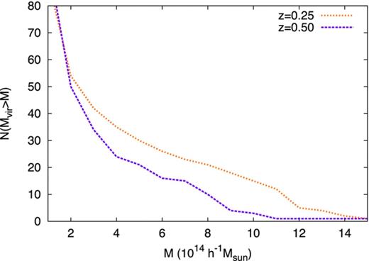
The cumulative virial-mass distribution of clusters in the sample at redshifts z = 0.25 (orange dotted curve) and z = 0.5 (purple dashed curve).
2.3 Relaxed clusters
If mergers between clusters take place along the line of sight the strong lensing efficiency can be enhanced. If the merger occurs across the sky, we will see multiple critical curves, which positively biases the cross-section for giant arcs. In the case that critical curves are merging, both the Einstein radii and the cross-section for giant arcs would be biased large. This could confuse our interpretation of the effects of baryon physics.
 , where
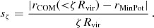
As a visual aid, the offset parameter for each cluster at z = 0.5 is shown in Fig. 0002 plotted against the aperture radius; each curve corresponds to an individual cluster. Any cluster for which the curve exceeds the dotted line (sζ = 0.1) for any radius in the given range is considered to be unrelaxed. Our adopted criterion to classify relaxed and unrelaxed clusters corresponds to similar definitions in the literature when we choose only one aperture radius, the virial radius, i.e. when we set ζ = 1 (e.g. Crone, Evrard & Richstone ; Thomas et al. ; D'Onghia & Navarro ; Neto et al. ; Power, Knebe & Knollmann ). However, we note that adopting this common choice we would be less sensitive to complex mass distributions near the core of a cluster, which is more important in the context of strong lensing. Our definition, in a sense, weights the disturbance caused by substructure by the inverse of radial position of the substructure. In order to verify whether there is any correlation within our sample between degree of relaxation and cluster mass, we plot in Fig. 0003 the positions of our clusters in the smax - Mvir plane. There is negligible correlation between the cluster's mass and the offset parameter that describes the degree of relaxation. The choice of threshold for smax above which a cluster is considered unrelaxed does not appear to bias the sample in terms of mass. The total sample of 42 clusters at z = 0.25 includes 17 relaxed clusters, and of the 34 clusters in total at z = 0.5, 14 are classified as relaxed. In Section and at the beginning of Section , we present the statistical results only for the relaxed subsample. In Section , we compare these results to those for unrelaxed clusters. For comparison, we note that if we had defined the relaxed subsample as those for which the offset at the virial radius is s1 < 0.07, as is common in the literature, we would have 23 relaxed clusters at z = 0.25 and 12 relaxed clusters at z = 0.5.

The offset parameter, sζ, as a function of aperture radius within which centre of mass is calculated, for all clusters at z = 0.5. The dotted horizontal line shows the value of the maximum offset parameter, smax = 0.1, allowed for a cluster to be classified as relaxed. Red and blue curves correspond to clusters which are then classified as unrelaxed and relaxed, respectively.
Relation between the maximum centre shift, smax, and the virial mass, Mvir, for all clusters. The orange circles represent clusters at z = 0.25, while the purple squares represent the clusters at z = 0.5.
3 CROSS-SECTION FOR GIANT Arcs

3.1 Calculating the lensing cross-section
 is the angular source position and
  is the angular position of the image on the sky. Producing maps of the deflection angle at each grid point requires a few steps, as shown in the schematic diagram in Fig. 0004. We describe the procedure below. The angular and spatial resolutions are quoted for sources at zs =2 and clusters at zL =0.25, but quantities for clusters at zL =0.5 are given in square brackets. The lensing mass is projected on to one of the two possible lens planes, depending on the position of the particles. Those that lie at a projected comoving distance of more than 0.9 h−1 Mpc [1.35 h−1 Mpc] from the cluster centre are placed on a low-resolution 2048 × 2048 grid. The angular resolution of this grid is 1.7 arcsec [0.9 arcsec]. Particles that are projected closer to the cluster core, and are therefore responsible for the bulk of the strong lensing, are placed on a high-resolution 2048 × 2048 grid. The angular resolution of this grid is 0.3 arcsec [0.2 arcsec]. The mass on each grid is smoothed with a truncated Gaussian filter of size σ = 5 h−1 kpc, to match the force-softening length of the simulation. The size of each grid is sufficiently larger than the projected extent of the mass on that grid, so that smoothing does not result in any loss of mass.
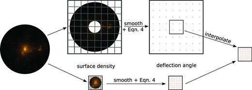
A schematic diagram describing the calculation of deflection angle,  , across a high-resolution grid. The lensing mass is divided into two parts: an inner and an outer region (shown in the bottom and top rows, respectively), each of which is projected on to a small high-resolution grid and a large low-resolution grid, respectively. The surface density distribution on each grid, κ, is smoothed and then the deflection angle is calculated using equation . The total deflection angle is the sum of these two. However, the deflection angle calculated in the inner region of the large grid must first be interpolated on to the small high-resolution grid. See the text for further details.
We convolve each of the two convergence maps with the appropriate kernel from equation . This leaves us with two maps of the deflection angle: one at high resolution where the deflection is solely due to the mass in the projected cluster core; the other at low resolution from the rest of the lensing mass. For the subsequent ray-shooting procedure, we use a single map of deflection angle for each cluster projection; the final map has the same size and resolution as the high-resolution grid described above. The deflection angle at each grid point is determined with bilinear interpolation from the closest grid points of the low-resolution map, and adding the corresponding grid point from the high-resolution map. The resulting deflection angle map has an angular resolution of 0.3 arcsec for clusters at zL =0.25 and 0.2 arcsec for clusters at zL =0.5.
Calculating the cross-section for giant arc formation requires a ray-shooting and arc-identifying procedure, which has been previously presented in Meneghetti et al. (, ). Elliptical sources with an equivalent radius of size 0.5 arcsec are placed throughout the source plane; more sources are placed in regions identified as caustics. The deflection angle maps allow mock images to be generated from the sources. The images are fitted to ellipses and the length-to-width ratio, L/W, is determined. If L/W surpasses some threshold elongation, η, the image is identified as a ‘giant arc’. The cross-section for giant arc formation, ση, is the area in the source plane covered by sources that are mapped on to giant arcs. For the present study, the L/W threshold is chosen to be η = 7.5 – following Puchwein et al. (), Mead et al. () and Meneghetti et al. () – because much larger cross-sections are subject to small number statistics, and much smaller cross-sections are too sensitive to the intrinsic ellipticities of the source galaxy. We discuss other choices of threshold of Section .
We present results in this section and Section for sources at redshift zs =2, but include the statistical results for a source redshift of zs =1 in Table 0001. For these lower source redshifts, we would expect smaller Einstein radii, so the deflection angle maps have a higher angular resolution: 0.2 arcsec for clusters at zL =0.25 and 0.1 arcsec for clusters at zL =0.5.
Statistical analysis of strong lensing properties of relaxed clusters. Column 1: simulation set. Columns 2 and 3: redshifts of the lens, zL, and of the source, zs. Column 4: Pearson correlation coefficient r for the log(σ7.5)–log(θE) relation. Columns 5 and 6: least-squares fit to the log(σ7.5)–log(θE) relation (see equation ). Column 7: typical value of the Einstein radius, θE, computed as the median value over 50 lines of sight through each cluster and then averaged over all clusters (units of arcseconds). Columns 8 and 9: values of  and
and  , defined as the lower and upper limits, respectively, of a true p-value from a KS test performed to compare the θE probability distribution of each simulation set against the corresponding result for the DM simulation. Column 10: the typical cross-section for the lensing of galaxies at zs into giant arcs with elongation η = 7.5, σ7.5, defined as the median value over 50 lines of sight through each cluster and then averaged over all clusters (units of 10−4 h−2 Mpc2). Columns 11 and 12: the same as in columns 8 and 9, respectively, but to compare the σ7.5 probability distribution
| Simulation | zL | zs | r | a | b | θE |  |  | σ7.5 |  |  |
| DM | 0.25 | 2 | 0.94 | 2.15 ± 0.02 | −6.04 ± 0.03 | 29 | – | – | 16 | – | – |
| NR | 0.25 | 2 | 0.92 | 1.93 ± 0.03 | −5.70 ± 0.04 | 30 | 0.02 | 1.00 | 17 | 0.11 | 1.00 |
| CSF | 0.25 | 2 | 0.97 | 2.02 ± 0.02 | −5.72 ± 0.03 | 33 | <10−5 | 0.87 | 24 | <10−5 | 0.35 |
| AGN | 0.25 | 2 | 0.97 | 2.11 ± 0.02 | −5.96 ± 0.03 | 30 | 1 × 10⁻⁴ | 1.00 | 18 | 3 × 10⁻⁴ | 1.00 |
| DM | 0.5 | 2 | 0.96 | 2.10 ± 0.02 | −5.90 ± 0.03 | 20 | – | – | 8.2 | – | – |
| NR | 0.5 | 2 | 0.95 | 2.08 ± 0.02 | −5.89 ± 0.03 | 21 | 0.11 | 1.00 | 8.9 | 0.14 | 1.00 |
| CSF | 0.5 | 2 | 0.96 | 1.87 ± 0.02 | −5.45 ± 0.03 | 21 | 7 × 10⁻⁵ | 1.00 | 12.4 | <10−5 | 0.59 |
| AGN | 0.5 | 2 | 0.96 | 2.09 ± 0.02 | −5.84 ± 0.03 | 21 | 0.93 | 1.00 | 10.6 | 0.07 | 1.00 |
| DM | 0.25 | 1 | 0.94 | 2.02 ± 0.02 | −5.92 ± 0.03 | 21 | – | – | 5.0 | – | – |
| NR | 0.25 | 1 | 0.91 | 1.81 ± 0.03 | −5.65 ± 0.04 | 22 | 0.008 | 1.00 | 5.6 | 0.16 | 1.00 |
| CSF | 0.25 | 1 | 0.96 | 2.10 ± 0.02 | −5.92 ± 0.03 | 25 | <10−5 | 0.80 | 10.5 | <10−5 | 0.11 |
| AGN | 0.25 | 1 | 0.95 | 2.18 ± 0.02 | −6.14 ± 0.03 | 22 | <10−5 | 0.99 | 6.1 | <10−5 | 1.00 |
| DM | 0.5 | 1 | 0.89 | 2.21 ± 0.04 | −6.13 ± 0.04 | 9 | – | – | 1.6 | – | – |
| NR | 0.5 | 1 | 0.88 | 2.29 ± 0.04 | −6.29 ± 0.05 | 10 | 4 × 10⁻⁴ | 1.00 | 1.5 | 0.20 | 1.00 |
| CSF | 0.5 | 1 | 0.93 | 2.02 ± 0.03 | −5.78 ± 0.03 | 12 | <10−5 | 0.46 | 2.9 | <10−5 | 0.25 |
| AGN | 0.5 | 1 | 0.92 | 2.32 ± 0.03 | −6.22 ± 0.04 | 10 | <10−5 | 0.95 | 2.2 | <10−5 | 0.99 |
| Simulation | zL | zs | r | a | b | θE | | | σ7.5 | | |
| DM | 0.25 | 2 | 0.94 | 2.15 ± 0.02 | −6.04 ± 0.03 | 29 | – | – | 16 | – | – |
| NR | 0.25 | 2 | 0.92 | 1.93 ± 0.03 | −5.70 ± 0.04 | 30 | 0.02 | 1.00 | 17 | 0.11 | 1.00 |
| CSF | 0.25 | 2 | 0.97 | 2.02 ± 0.02 | −5.72 ± 0.03 | 33 | <10−5 | 0.87 | 24 | <10−5 | 0.35 |
| AGN | 0.25 | 2 | 0.97 | 2.11 ± 0.02 | −5.96 ± 0.03 | 30 | 1 × 10⁻⁴ | 1.00 | 18 | 3 × 10⁻⁴ | 1.00 |
| DM | 0.5 | 2 | 0.96 | 2.10 ± 0.02 | −5.90 ± 0.03 | 20 | – | – | 8.2 | – | – |
| NR | 0.5 | 2 | 0.95 | 2.08 ± 0.02 | −5.89 ± 0.03 | 21 | 0.11 | 1.00 | 8.9 | 0.14 | 1.00 |
| CSF | 0.5 | 2 | 0.96 | 1.87 ± 0.02 | −5.45 ± 0.03 | 21 | 7 × 10⁻⁵ | 1.00 | 12.4 | <10−5 | 0.59 |
| AGN | 0.5 | 2 | 0.96 | 2.09 ± 0.02 | −5.84 ± 0.03 | 21 | 0.93 | 1.00 | 10.6 | 0.07 | 1.00 |
| DM | 0.25 | 1 | 0.94 | 2.02 ± 0.02 | −5.92 ± 0.03 | 21 | – | – | 5.0 | – | – |
| NR | 0.25 | 1 | 0.91 | 1.81 ± 0.03 | −5.65 ± 0.04 | 22 | 0.008 | 1.00 | 5.6 | 0.16 | 1.00 |
| CSF | 0.25 | 1 | 0.96 | 2.10 ± 0.02 | −5.92 ± 0.03 | 25 | <10−5 | 0.80 | 10.5 | <10−5 | 0.11 |
| AGN | 0.25 | 1 | 0.95 | 2.18 ± 0.02 | −6.14 ± 0.03 | 22 | <10−5 | 0.99 | 6.1 | <10−5 | 1.00 |
| DM | 0.5 | 1 | 0.89 | 2.21 ± 0.04 | −6.13 ± 0.04 | 9 | – | – | 1.6 | – | – |
| NR | 0.5 | 1 | 0.88 | 2.29 ± 0.04 | −6.29 ± 0.05 | 10 | 4 × 10⁻⁴ | 1.00 | 1.5 | 0.20 | 1.00 |
| CSF | 0.5 | 1 | 0.93 | 2.02 ± 0.03 | −5.78 ± 0.03 | 12 | <10−5 | 0.46 | 2.9 | <10−5 | 0.25 |
| AGN | 0.5 | 1 | 0.92 | 2.32 ± 0.03 | −6.22 ± 0.04 | 10 | <10−5 | 0.95 | 2.2 | <10−5 | 0.99 |
Statistical analysis of strong lensing properties of relaxed clusters. Column 1: simulation set. Columns 2 and 3: redshifts of the lens, zL, and of the source, zs. Column 4: Pearson correlation coefficient r for the log(σ7.5)–log(θE) relation. Columns 5 and 6: least-squares fit to the log(σ7.5)–log(θE) relation (see equation ). Column 7: typical value of the Einstein radius, θE, computed as the median value over 50 lines of sight through each cluster and then averaged over all clusters (units of arcseconds). Columns 8 and 9: values of and , defined as the lower and upper limits, respectively, of a true p-value from a KS test performed to compare the θE probability distribution of each simulation set against the corresponding result for the DM simulation. Column 10: the typical cross-section for the lensing of galaxies at zs into giant arcs with elongation η = 7.5, σ7.5, defined as the median value over 50 lines of sight through each cluster and then averaged over all clusters (units of 10−4 h−2 Mpc2). Columns 11 and 12: the same as in columns 8 and 9, respectively, but to compare the σ7.5 probability distribution
| Simulation | zL | zs | r | a | b | θE | | | σ7.5 | | |
| DM | 0.25 | 2 | 0.94 | 2.15 ± 0.02 | −6.04 ± 0.03 | 29 | – | – | 16 | – | – |
| NR | 0.25 | 2 | 0.92 | 1.93 ± 0.03 | −5.70 ± 0.04 | 30 | 0.02 | 1.00 | 17 | 0.11 | 1.00 |
| CSF | 0.25 | 2 | 0.97 | 2.02 ± 0.02 | −5.72 ± 0.03 | 33 | <10−5 | 0.87 | 24 | <10−5 | 0.35 |
| AGN | 0.25 | 2 | 0.97 | 2.11 ± 0.02 | −5.96 ± 0.03 | 30 | 1 × 10⁻⁴ | 1.00 | 18 | 3 × 10⁻⁴ | 1.00 |
| DM | 0.5 | 2 | 0.96 | 2.10 ± 0.02 | −5.90 ± 0.03 | 20 | – | – | 8.2 | – | – |
| NR | 0.5 | 2 | 0.95 | 2.08 ± 0.02 | −5.89 ± 0.03 | 21 | 0.11 | 1.00 | 8.9 | 0.14 | 1.00 |
| CSF | 0.5 | 2 | 0.96 | 1.87 ± 0.02 | −5.45 ± 0.03 | 21 | 7 × 10⁻⁵ | 1.00 | 12.4 | <10−5 | 0.59 |
| AGN | 0.5 | 2 | 0.96 | 2.09 ± 0.02 | −5.84 ± 0.03 | 21 | 0.93 | 1.00 | 10.6 | 0.07 | 1.00 |
| DM | 0.25 | 1 | 0.94 | 2.02 ± 0.02 | −5.92 ± 0.03 | 21 | – | – | 5.0 | – | – |
| NR | 0.25 | 1 | 0.91 | 1.81 ± 0.03 | −5.65 ± 0.04 | 22 | 0.008 | 1.00 | 5.6 | 0.16 | 1.00 |
| CSF | 0.25 | 1 | 0.96 | 2.10 ± 0.02 | −5.92 ± 0.03 | 25 | <10−5 | 0.80 | 10.5 | <10−5 | 0.11 |
| AGN | 0.25 | 1 | 0.95 | 2.18 ± 0.02 | −6.14 ± 0.03 | 22 | <10−5 | 0.99 | 6.1 | <10−5 | 1.00 |
| DM | 0.5 | 1 | 0.89 | 2.21 ± 0.04 | −6.13 ± 0.04 | 9 | – | – | 1.6 | – | – |
| NR | 0.5 | 1 | 0.88 | 2.29 ± 0.04 | −6.29 ± 0.05 | 10 | 4 × 10⁻⁴ | 1.00 | 1.5 | 0.20 | 1.00 |
| CSF | 0.5 | 1 | 0.93 | 2.02 ± 0.03 | −5.78 ± 0.03 | 12 | <10−5 | 0.46 | 2.9 | <10−5 | 0.25 |
| AGN | 0.5 | 1 | 0.92 | 2.32 ± 0.03 | −6.22 ± 0.04 | 10 | <10−5 | 0.95 | 2.2 | <10−5 | 0.99 |
3.2 The impact of baryons on the cross-section for giant arcs
The baryonic processes as implemented in the hydrodynamical simulations affect the details of the structure of each cluster halo. Fig. 0005 shows a single cluster of mass Mvir = 8 × 10¹⁴ h−1 M⊙ in our zL =0.5 sample as found in each of the four resimulations. The basic structure is recognizable in each simulation and the subhaloes appear in much the same positions, as seen in the convergence maps along the top row. However, the distribution of matter near the clusters’ centre is sufficiently altered by baryonic physics so that the caustics, as shown in the bottom row of the same figure, are distinct. In particular, note that the CSF simulation produces larger source caustics, shown in blue, and larger tangential image caustics – or critical curves – shown in red. The tangential part of the image caustic extends around a substructure that was subcritical in the other simulations. For this particular cluster, as seen from one line of sight, the strong lensing efficiency is the highest when the cluster is generated within the CSF simulation.

One cluster at zL =0.5 seen from the same viewpoint within different simulations: DM (left-hand panel), NR (second panel), CSF (third panel) and AGN (right-hand panel). Along the top row, we show the convergence map of the cluster, ∼410 arcsec across, in which brighter regions represent higher surface densities; along the bottom row is the corresponding source caustic in blue and image caustic, also known as the critical curve, in red, both determined for a source at redshift zs =2.
It is our aim to determine whether this is generally true for simulated galaxy clusters, and in particular, how the strong lensing properties predicted by the AGN simulations compare with the other simulations. We have a large sample of galaxy cluster, but we should not consider only one line of sight through each cluster. Due to the aspherical nature of clusters, as well as the presence of substructure, each line of sight produces a unique cross-section. Therefore, each cluster is associated with a distribution of possible cross-sections (see e.g. fig. 3 of Dalal, Holder & Hennawi ). In Fig. 0006, we show such a distribution by measuring the cross-section, σ7.5, for 50 lines of sight through one cluster in our sample, also seen in Fig. 0005. In the present study, we analyse projections of each cluster along 50 randomly chosen lines of sight. The results for all our sets of simulated clusters are combined in the left-hand panel of Fig. 0007.
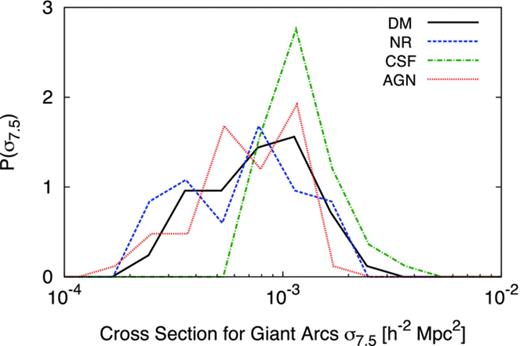
The probability distributions for the cross-section that would be measured for a single simulated cluster at zL =0.5 for a source redshift of zs =2; the cluster is the same as that shown in Fig. 0005. Different curves refer to the distributions produced by the four different simulations: DM (black solid line), NR (blue dashed line), CSF (green dash–dotted line) and AGN (red dotted line).
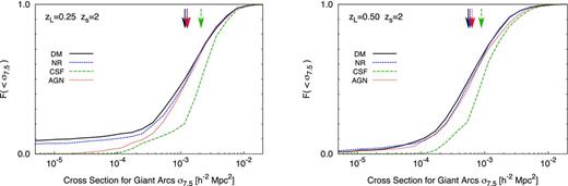
The cumulative probability distribution for the source-plane cross-section for the formation of giant arcs combining 50 lines of sight through the relaxed clusters at zL =0.25 (left-hand panel) and zL =0.5 (right-hand panel). Different lines and colours have the same meaning as in Fig. 0006. The arrows mark the median values of the σ7.5 cross-section for the models.
We conduct a two-sample Kolmogorov–Smirnov (KS) test to compare the probability distribution of σ7.5 values for each simulation against the same distribution for the DM simulations. The D-statistic is the maximum difference between the two cumulative probability distributions. Ideally, we would like to determine the probability, pσ, that the D-statistic would be at least as large as that measured assuming the samples are drawn from the same underlying distribution. We recognize that while the clusters are independent, the many lines of sight analysed for each cluster are not independent of each other. In an actual observational sample, one would measure a single strong lensing efficiency for each cluster; however, using a simulated sample, scatter due to orientation has to be taken into account. Therefore, stacking the results for all lines of sight analysed, we calculate the D-statistic. Using the total number of lines of sight (50 times the number of clusters) as the ‘sample size’ provides a lower limit for the p-value,  . Alternatively, by letting the number of clusters to be the ‘sample size’, we can obtain an upper limit on the p-value,
  . Both are listed in Table 0001. If the clusters were all perfectly symmetrical, so that all lines of sight resulted in the same value of σ7.5, then
  would be equivalent to the required pσ.
Table 0001 also include the typical cross-sections for clusters in each simulation, for low and high source redshifts: zs =1 and 2. These are calculated by taking the median value of the cross-section over the 50 lines of sight analysed for each cluster and then averaging over all clusters. Comparing the results for DM and NR simulations, we find that the ability to lens background galaxies into giant arcs is similar, independent of whether the cluster lens is simulated with collisionless particles only, or with additional non-radiative gas. As seen for the CSF simulation, when cooling and star formation are implemented, the cross-section for the formation of giant arcs is boosted by a factor of ∼1.5 for high source redshifts (zs =2) and ∼2 for lower source redshifts (zs =1). This is a slightly smaller ‘boost’ relative to the findings of Puchwein et al. (), Rozo et al. () and Mead et al. (). This difference with respect to previous simulation models can be understood in terms of the more efficient SN feedback implemented in our CSF simulation set, which more efficiently counteracts the effect of halo contraction induced by cooling. In fact, Puchwein et al. () use the same model for galactic ejecta, but with a smaller velocity of galactic winds, with vw =350 km s−1. Furthermore, Rozo et al. () and Mead et al. () only include thermal schemes for SN feedback, which are rather inefficient in regulating cooling at the centre of cluster-sized haloes.
AGN feedback reduces the giant-arc cross-section and makes it comparable to the predicted cross-section from collisionless simulations. When we compare clusters modelled with DM only (DM results shown in black) and their counterparts modelled with the complete set of baryonic processes, including AGN feedback (AGN shown in red), we find surprisingly little difference in the typical cross-sections for clusters at zL =0.25 – now a boost of only ∼10 per cent. However, at zL =0.5 clusters modelled with AGN feedback are ∼30 per cent more efficient at lensing background galaxies into giant arcs. Given the results for Einstein radii (see Section ), this is likely due to the presence of substructures that produce additional arcs rather than the redistribution of mass near the cluster centre. The difference in the results between CSF and the AGN simulations arise from a combination of the reduced SN wind speed and the introduction of thermal AGN feedback. However, if the CSF simulations had a similarly reduced wind speed, the reduced feedback efficiency would lead to increased cooling and a higher lensing cross-section, therefore it is the AGN feedback that is responsible for reducing the lensing efficiency. Mead et al. () analysed three projections for each of the five clusters at zL =0.2 with similar simulation sets. For four of these five clusters, the strong lensing cross-sections for the DM simulation and their AGN simulation were very similar. At this redshift, given the small sample and number of projections, this is consistent with our findings.
As described earlier, images are identified as arcs if their L/W surpasses the threshold elongation η. Although extreme values for this threshold are not useful, the exact value is somewhat arbitrarily chosen; to be sure that the results are not qualitatively affected by this choice, we plot the cross-section as a function of η in Fig. 0008. The lines represent the median cross-section over the 50 lines of sight for each individual cluster and then averaged over all the clusters in the (relaxed) sample. The error bars represent the 16th and 84th percentiles for individual clusters and then averaged over all the clusters. These error bars, therefore, reflect the triaxiality of the clusters. Unsurprisingly, a larger and more extreme choice of threshold allows a smaller cross-section, since less sources would be able to produce such long and thin arcs, but the qualitative differences between the different simulation sets are the same.
The giant-arc cross-section plotted against the chosen elongation threshold η for the relaxed cluster subsample at zL =0.25 (left-hand panels) and zL =0.5 (right-hand panels). The cross-section for a given value of η is the median of 50 lines of sight through each cluster and then averaged over all clusters. The error bars mark the 16th and 84th percentiles for each cluster and then averaged over all clusters. The source redshift is zs =2.
By comparing the error bars in Fig. 0008 for all resimulations, we find that as in Rozo et al. (), the spread in the distribution of possible cross-sections is also reduced significantly in the CSF simulations. These clusters are less susceptible to line-of-sight effects than those modelled with DM only or non-radiative gas, predominantly due to the more spherical shape of the clusters resulting from the condensing of baryons and the subsequent response from the DM component (Blumenthal et al. ; Gnedin et al. ; Kazantzidis et al. ; Bryan et al. ). The steeper inner profile (see Section ) makes the clusters less susceptible to coincidental mass along the line of sight. Although AGN feedback regulates the isotropic condensation of baryons, the reduced spread in cross-sections is also found for the AGN clusters, particularly at zL =0.5.
Fig. 0009 shows the giant-arc cross-section, σ7.5, plotted against the mass of each cluster. Each cluster is represented as a single point in the graph, with different colours representing the counterparts in the four resimulations. The error bars mark the 16th and 84th percentiles of σ7.5 found over the 50 lines of sight analysed. The figure suggests that there exists a scaling relation between lensing efficiency and mass, but that the correlation is tighter at higher overdensities; this reflects the region most responsible for strong lensing. The higher scatter when σ7.5 is plotted as a function of M500 reflects the fact that different resimulations create differing distributions of baryons in the cluster core, when comparing clusters at a fixed mass at lower overdensities.
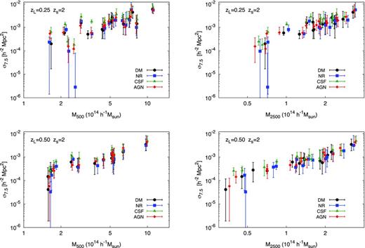
The cross-section for the formation of giant arcs at source redshift of zs =2 as a function of cluster mass, for our relaxed cluster subsample. Each dot represents the median cross-section from the 50 lines of sight analysed for a single cluster, while the error bars mark the 16th and 84th percentiles. In the left-hand panels the characteristic mass is M500, while for the right-hand panels the characteristic mass is M2500. The clusters at zL =0.25 are shown in the top row, while the clusters at zL =0.5 are shown in the bottom row.
4 Einstein RADII
The cosmological test based on arc statistics is subject to uncertainty in the characteristics of the source population. Performing a comparison with observed arc statistics requires one to convolve the predicted giant-arc cross-section with an assumed redshift distribution for the background galaxies. The uncertainties in this redshift distribution create an additional uncertainty in the cosmological test. This additional uncertainty is unnecessary since one might instead characterize strong lensing efficiency by the angular scale which separates highly magnified images; this is known as the Einstein radius. Measuring the Einstein radii requires the observer to measure the shape and redshift of a reasonable number of highly magnified high-redshift sources, reconstruct the lens mass distribution, and infer the critical curves at a single redshift. This is achievable even if the various sources are at different redshifts, and bypasses the need to independently measure the expected number density and redshift evolution of the sources. We therefore measure the Einstein radii for our cluster sample and compare the results between the different resimulations.
4.1 Measuring the Einstein radius
The angular separation of highly magnified background galaxies has a formal definition, which is strictly applicable only in the case of axially symmetric lenses. However, galaxy clusters are not axially symmetric in general; there exist a number of different definitions in the literature for how one might calculate the Einstein radius for more realistic lenses. For example, one might divide the area enclosed within the tangential critical curve by π, as per the so-called ‘equivalent Einstein radius’ definition used, e.g. by Puchwein & Hilbert (), Zitrin et al. () and Redlich et al. (). On the other hand, Broadhurst & Barkana () define the ‘effective Einstein radius’ as the radius that encloses a mean surface density equal to the critical surface density κ = 1 (see Puchwein & Hilbert for further discussion on how these two definitions compare). We, instead, follow the definition of Meneghetti et al. () and characterize our statistics by a ‘median Einstein radius’: the median distance of the tangential critical points from the clusters centre. Meneghetti et al. () have demonstrated that the median Einstein radius has a tighter correlation with strong lensing cross-section than the ‘equivalent Einstein radius’. When measuring the Einstein radius, Meneghetti et al. () define the cluster centre to be the location of the maximum of the projected mass distribution. In the present work, we define the centre to be the projected position of the particle in the simulated cluster with the lowest potential. This is done in order to avoid attributing the position of the centre to a subhalo in cases in which such a subhalo is fortuitously projected, so it has a higher projected mass density than the centre of the main halo.
We use the high-resolution deflection-angle map (as described in Section ) to identify tangential critical points within the same field of view at the same angular resolution. There can be complications in the presence of substructure, which require one to discard some of the critical points before measuring the Einstein radius. We show an unrelaxed cluster in Fig. 0010 as an example. There is a large substructure present and, from some lines of sight, visible within the field of view. For each line of sight analysed, critical points are mapped out across the lens plane forming a ‘critical curve’ also known as an image caustic; these correspond to the caustics in red. Then, critical points associated with the tangentially sheared images (as opposed to radially sheared) at the ‘primary’ critical curve around the centre of the cluster are identified, so that ‘secondary’ critical curves associated with substructure do not bias the measurement. These are the ‘cleaned’ curves shown in black. The projected distance of each ‘clean’ point from the cluster centre is measured; the Einstein radius, θE, is the median value over all these points.
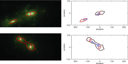
The surface density map (left-hand panels) and image and source caustic (right-hand panels) of an unrelaxedzL =0.5 cluster in our sample. In the left-hand panels, brighter regions correspond to higher surface density and the image caustic is overlaid in red. In the right-hand panels, the image caustic is shown in red, with the ‘cleaned’ caustic – used to infer the Einstein radius – drawn in black, and the source caustic at zs =2 shown in blue. The ‘primary’ image caustic is associated with the centre of the cluster, while a large substructure present within the field of view produces a ‘secondary’ image caustic. Seen from one line of sight (top row), the secondary caustic is distinct, so the cleaned caustic captures only the primary caustic, while from the other line of sight (bottom row) the primary and secondary caustics are merged, so the cleaned caustic captures both, and artificially enhances the inferred Einstein radius.
If the secondary critical curve merges with the primary, as shown in the bottom row of Fig. 0010, they cannot be distinguished, and θE is artificially increased. The cross-section σ7.5 gives, to a first approximation, the region enclosed by the source caustics (shown in blue). The measurement of σ7.5 can be artificially enhanced by the presence of substructure. We discuss this further in Section . For a relaxed cluster, there would be fewer lines of sight in which the secondary and primary critical curves merge, and the cluster will have smaller secondary critical curves which have a less significant impact on the measurement of σ7.5 and θE.

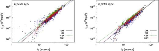
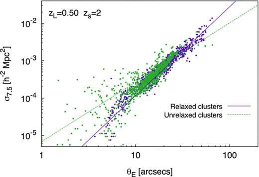
Relationship between the giant-arc cross-section, σ7.5, and the Einstein radius, θE, for each of the 50 orientations of each cluster. In the left-hand panel, we show the results from the clusters at zL =0.25, and in the right-hand panel, we show the results from the clusters at zL =0.5; both are for source redshift of zs =2. Results for the four simulations are combined: DM only (black), DM and non-radiative gas (blue), with cooling and star formation (green) and with AGN feedback (red).
We can expect the slope of the log(σ7.5)–log(θE) relation to reflect the inner mass profile of the lens (Redlich et al. ). DM haloes, such as those in DM simulations, follow Navarro–Frenk–White (NFW) profiles (Navarro, Frenk & White ), with inner density profiles that fall off as ρ(r) ∝ r−1. In clusters with significant gas cooling, such as those in the CSF simulations, the density profile is close to isothermal (ρ ∝ r−2), and so produce a large tangential magnification relative to radial magnification, and therefore a boost in σ7.5 compared to the DM clusters. Since the positions of the critical points are relatively stable to the inner slope – assuming no significant redistribution of mass to larger radii – there is a greater boost in the giant-arc cross-section as opposed to the Einstein radius, particularly for low-mass lenses (see fig. 5.7 in Oguri ), which results in a shallower slope in the log(σ7.5)–log(θE) relation, and a smaller value of a. For low source redshifts, lensing efficiencies are lower, resulting in greater scatter as the source sizes approach the resolution of the lensing maps; the line of best fit is sensitive to this scatter and less sensitive to the inner mass profiles.
4.2 The impact of baryons on the Einstein radii
We plot the cumulative probability distribution for Einstein radii in Fig. 0012 combining all 50 lines of sight through each of the relaxed clusters. As given in Section , we conduct a two-sample KS test to compare the probability distribution for each simulation against the DM simulation. We want to determine the probability, pθ, that the D-statistic would be at least as large as that measured assuming the samples are drawn from the same underlying distribution. As noted before, while the clusters are independent, the many lines of sight analysed for each cluster are not independent of each other. However, for the simulated sample, scatter due to orientation has to be taken into account. Stacking the results for all lines of sight analysed, we calculate the D-statistic. Defining the ‘sample size’ as the total number of lines of sight (50 times the number of clusters) provides a lower limit for the p-value,  . Alternatively, by letting the number of clusters to be the ‘sample size’, we can obtain an upper limit on the p-value,
  . Both are listed in Table 0001.
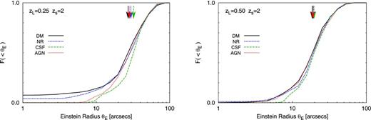
The cumulative distribution of Einstein radii obtained by combining 50 lines of sight through each of the relaxed clusters in the sample. The source redshift is assumed here to be zs =2. In the left-hand panel, we show the results for the 24 relaxed clusters with Mvir > 3 × 10¹⁴ h−1 M⊙ at redshift zL =0.25. In the right-hand panel, we show the results for the 18 relaxed clusters above the same mass limit at redshift zL =0.5.
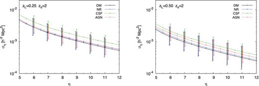
Table 0001 also includes the typical Einstein radii for clusters in each simulation, for low and high source redshifts: zs =1 and 2. These are calculated by taking the median value of the Einstein radius over the 50 lines of sight analysed for each cluster and then averaging over all clusters. The strong lensing efficiency of a cluster is sensitive to the enclosed mass within θE. Therefore, lens–source configurations that produce larger Einstein radii are less susceptible to the effects of baryons, since AGN lead to the redistribution of mass within reasonably small radii; we leave a more detailed discussion to Section . Comparing the results for DM and NR simulations, we find that Einstein radii are similar whether the cluster lens is simulated with collisionless particles only or with additional non-radiative gas. Comparing the results for DM and CSF simulations, gas cooling and star formation increase the predicted Einstein radii by ∼10 per cent for high source redshifts (zs =2) and ∼20–40 per cent for lower source redshifts (zs =1). This effect is more significant for lower source redshifts for which the Einstein radii are typically smaller. With the inclusion of AGN feedback, the typical Einstein radii are reduced with respect to the CSF case. For Einstein radii calculated for source redshifts of zs =2, the fractional increase relative to the clusters in the DM simulations is only ∼5 per cent. This is the source redshift that reconstructed critical curves are commonly scaled to in observational studies. The greatest difference between the predicted Einstein radii from DM and AGN simulations occurs for high-z clusters and low-z sources, which corresponds to the smaller Einstein radii (θ < 20 arcsec).
Fig. 0013 shows the Einstein radius for each cluster as a function of its mass. We plot the median value of θE measured over the 50 lines of sight for an individual cluster; the error bars, denoting the 16th and 84th percentiles, reflect a measure of spread associated with the line-of-sight variance. We note that one of the clusters has an unusually large scatter in θE associated with the different orientations. This cluster has a small Einstein radius and is probably on a similar scale to angular resolution. The cluster mass is measured at two different overdensities: Δ = 500 and 2500. The Einstein radius increases with cluster mass, as expected, but the correlation is tighter at higher overdensities. This is in line with the expectation that high overdensities are responsible for strong lensing. The Einstein radius for a fixed value of M500 is slightly larger for clusters in the CSF simulations due to the higher concentration of these clusters. The asphericity, reflected in the size of the error bars, is also smaller for clusters in these simulations.
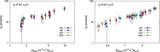
The Einstein radius for a source redshift of zs =2 versus cluster mass combining 50 lines of sight through the relaxed clusters at zL =0.5. For the left-hand panels, the characteristic mass is M500, while for the right-hand panels, the characteristic mass is M2500.
4.3 Unrelaxed clusters
Unrelaxed clusters produce highly complex caustic structures which are the consequence of high-mass subhaloes that lie within the field of view. These can create non-trivial complications in measurements of both the giant-arc cross-section and the Einstein radius. In the previous sections, we have discussed the lensing properties of relaxed clusters so as not to be susceptible to the effects of massive substructures. We now consider the subsample of unrelaxed clusters to verify how their properties differ and how they would affect lensing predictions. We remind the reader that at zL =0.25 there are 25 unrelaxed clusters and at zL =0.5 there are 20 unrelaxed clusters in our sample. Fig. 0014 shows the correlation between σ7.5 and θE for clusters in the DM simulation comparing the relaxed and unrelaxed subsamples. The unrelaxed clusters in our sample would introduce a large scatter. We verify that as the threshold for the unrelaxedness parameter smax is increased, the scatter increases in the relaxed subsample. This is primarily due to giant arcs associated with substructure which induce a positive bias on the calculation of σ7.5. The Pearson correlation coefficient, r, for unrelaxed clusters in all simulations ranges from 0.87 to 0.92 at zL =0.25 and from 0.82 to 0.90 at zL =0.5.
The relationship between the giant-arc cross-section, σ7.5, and the Einstein radius, θE, for each of the 50 lines of sight analysed for each relaxed cluster in the DM simulation at zL =0.5, for a source redshift of zs =2. Results for relaxed clusters are shown in purple (solid line of best fit), while the unrelaxed clusters are shown in green (dotted line of best fit). The unrelaxed subsample exhibits a larger intrinsic scatter.
The scatter above the σ7.5–θE lines of best fit is primarily because of substructures that are large enough to produce distinct caustics (see the top row in Fig. 0010), which induce a positive bias on the cross-section; as long as the caustics associated with projected substructures are well separated from the primary caustic, the Einstein radius measurement is not affected. On the other hand, if substructures are projected near the clusters centre, their caustics merge and produce highly elongated, critical curves (see the bottom row in Fig. 0010); this artificially increases the Einstein radius more than the cross-section, thus down-scattering results for unrelaxed clusters with respect to the σ7.5–θE lines of best fit obtained for relaxed clusters.
Fig. 0015 shows the cumulative probability distribution of Einstein radii for the unrelaxed subsample. Clusters identified as unrelaxed are more likely to be merging systems in which the main lens has a significantly lower mass than the total mass within the system. Hence, we find that typical Einstein radii are only 50–70 per cent of the size of Einstein radii for the relaxed counterparts.
The probability distribution for Einstein radii combining 50 lines of sight through each of the unrelaxed clusters in the sample. The source redshift is zs =2. In the left-hand panel, we show the results for clusters at zL =0.25; in the right-hand panel, we show the results for clusters at redshift zL =0.5.
We may now consider whether the effect of baryons on strong lensing properties is similar for the relaxed and unrelaxed subsamples. Gas cooling and star formation produce clusters with a higher mass concentration; unrelaxed clusters have more substructures, which are also more compact than their collisionless counterparts (see e.g. the substructures visible in the cluster shown in Fig. 0005). Therefore, the unrelaxed clusters in the CSF simulations have larger primary caustics than their DM counterparts, but, compared to relaxed clusters, are also more likely to host secondary caustics that merge with the primary and boost the Einstein radius. Thus, the Einstein radii at zs =2 for clusters in the CSF simulations are higher by ∼20 per cent than for their collisionless counterparts. This boost increases to ∼50–70 per cent when we measure the Einstein radii at lower source redshifts. This is significantly larger than the boost for relaxed clusters.
The introduction of AGN feedback once again reduces the strong lensing efficiency of unrelaxed clusters; the Einstein radii at zs =2 for unrelaxed clusters in the AGN simulations are only 5 per cent larger than those for their collisionless counterparts in the DM simulations. The difference in strong lensing efficiency is essentially the same for both relaxed and unrelaxed clusters. However, a mixed sample – with both relaxed and unrelaxed clusters – would have smaller Einstein radii on average, than a relaxed-only sample.
4.4 Cluster mass profiles
In the previous sections, we have seen that gas cooling, star formation and stellar and AGN feedback have varying and often counteracting effects on strong lensing efficiencies. Here, we look at the mass profiles of the cluster haloes to trace the origin of the change in strong lensing properties. However, a detailed analysis of the mass profile fitting and the effect of baryons on the concentration–mass relation is beyond the scope of this paper.
Previous analyses of non-radiative simulations in the literature have found that the gas profiles exhibit cores (e.g. Rasia, Tormen & Moscardini ; Rudd et al. ). Fig. 0016 shows the spherically averaged differential density profile for the relaxed clusters in two of our simulations: CSF and AGN. The profiles are shown for different components: dark matter, dark matter and gas, dark matter and gas and stars. The shaded regions mark the cluster-to-cluster scatter, while the error bars mark the error of the mean; the small size of the error bars reflect the consistency in the profiles across the clusters.
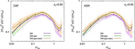
The differential density profile of DM (purple); DM and gas (green); DM, gas and stars (yellow). Clusters included in analysis are the relaxed subsample at zL =0.5 in the CSF simulation (left-hand panel) and the AGN simulation (right-hand panel). The solid lines represent the average over all clusters, the shaded regions (in the respective colours) are between the 16th and 84th percentiles among the clusters, while the error bars correspond to the estimated error of the mean. The profile for each cluster has been normalized to the average mass density within the virial radius, and scaled with the square of the radius in order to reduce the dynamic range.
In keeping with previous analyses, we confirm that within r ≲ 0.1Rvir gas cooling and star formation steepen the total mass profile with respect to DM-only simulations. In both CSF and AGN simulations, the baryonic component is dominated by stars within r ≲ 0.1Rvir; the gas component has a core and is distributed primarily beyond 10 per cent of the virial radius. The steepening of the inner profile is associated with the build-up of stellar mass; AGN heating regulates star formation and therefore reduces the inner slope. We have mentioned earlier that comparisons between these two simulations must be interpreted carefully given that in the AGN simulations SN wind speeds are increased while simultaneously introducing AGN feedback. Interestingly, Duffy et al. () have shown that in simulations without AGN feedback, the inner slope of the DM profile of clusters at z = 0 actually steepens slightly when the SN wind speed is reduced, but the stellar fraction within r < 0.05Rvir is increased significantly, which we might expect to lead to an overall increase in the inner slope of the total mass profile. They find that the introduction of AGN feedback reduces both the stellar fraction within r < 0.05Rvir and the inner slope of the DM profile. Our findings are in agreement with Duffy et al. () as well as several previous studies (e.g. Gnedin et al. ; Puchwein et al. ; Mead et al. ; Martizzi et al. ), in which the simulated clusters are analysed at z ≲ 0.3. In our analysis, we also included clusters identified at higher redshift, z = 0.5, and found no strong redshift dependence of the results.
In order to see how the redistribution of baryons affects the strong lensing, it is helpful to analyse the cumulative mass within different radii. In Fig. 0017, we show the cumulative mass profiles for the clusters at zL =0.25 and 0.5, respectively. The smallest radius shown corresponds to 1 per cent of the virial radius, which corresponds to 16 h−1 kpc for the smallest virial radius of all the clusters, or at least three times the softening length.
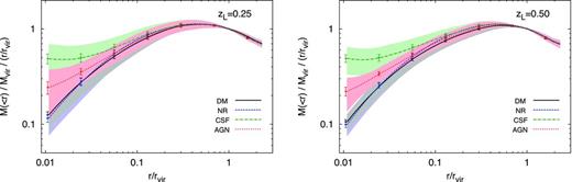
The cumulative mass profile for the relaxed clusters at zL =0.25 (left-hand panel) and zL =0.5 (right-hand panel). The lines reflect the average profile stacking all the clusters, while the shaded regions are between the 16th and 84th percentiles among the clusters. The profile for each cluster has been normalized to the virial mass, and scaled with the radial distance in order to reduce the dynamic range.
Our non-radiative NR simulations generate clusters with slightly more mass within r < 0.1Rvir than their DM counterparts; however, this is too mild to produce significantly stronger lenses in agreement with the findings of Rozo et al. () and Puchwein et al. (). The CSF simulations produce clusters that contain significantly more mass within r < 0.1Rvir (see also Gnedin et al. ; Puchwein et al. , for comparable results on steepening of density profiles in radiative simulations). However, these simulations suffer the ‘overcooling’ problem – on average, 22 per cent of the baryonic mass within r500 in CSF clusters is in the form of stars – thus implying that the corresponding boost in strong lensing efficiency ought to be unrealistic. A more detailed comparison between simulation and observation results on the stellar fraction will be presented by Planelles et al. (in preparation).
AGN feedback reduces the total mass within 0.1Rvir for clusters at both redshifts. If we compare the DM and AGN simulations, we note that including AGN feedback results in clusters that contain more mass within r < 0.03Rvir relative to their collisionless counterparts. However, this does not translate into larger strong lensing efficiencies. The reason for this is seen in Fig. 0018 which shows the fraction of the virial radius encompassed by the Einstein radius at the cluster redshift, as a function of cluster mass. Typical Einstein radii are larger than the radius within which enclosed mass is affected by baryonic physics. However, while clusters in the AGN simulations have a different structure with respect to their DM counterparts, this difference does not produce stronger lenses, for sources at zs =2. If we consider the results for sources at zs =1, as shown in Table 0001, the typical Einstein radii are smaller than for sources at zs =2. As a consequence, there is a higher significance to the probability that clusters in the CSF simulations are stronger lenses than their DM counterparts. Still, the strong lensing properties of clusters in the AGN simulations are still fairly consistent with the DM counterparts.
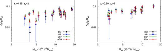
The Einstein radius relative to the cluster radius as a function of cluster mass. For each cluster, the median of the 50 analysed lines of sight is plotted with error bars reflecting the 16th and 84th percentiles over the distribution of lines of sight. In the left-hand panel, we show relaxed clusters at zL =0.25, while relaxed clusters at zL =0.5 are in the right-hand panel.
We defer a more detailed comparison with observations, extending the simulated cluster sample to a wider range of masses, to a future study. For the purpose of the present study, it is sufficient to say that the suppression of star formation due to gas heating by AGN feedback in the AGN simulations is responsible for the decrease in total mass in the cluster core, and subsequently, the decrease in the strong lensing efficiency of these clusters compared to their counterparts in the CSF simulations.
5 CONCLUSIONS
In the present study, we have analysed the strong lensing efficiency of about 15 relaxed simulated clusters at zL =0.25 and 0.5. The clusters were resimulated under a number of different physical models: DM only (DM); non-radiative gas (NR); cooling, star formation, SN feedback (CSF); and additional AGN feedback (AGN). Our main findings are as follows.
There are no significant differences in the strong lensing properties and density profiles of clusters modelled with DM only and those that include a non-radiative gas component.
Gas cooling and star formation have the effect of increasing the giant arc counts and Einstein radii even in the presence of stellar feedback, which can push gas out of galaxies and reduce star formation.
When AGN feedback is included in the simulations, the strong lensing efficiency of the clusters is significantly reduced. Einstein radii at zs =2 are only 5 per cent larger than those for the DM counterparts, a boost that is increased to 10–20 per cent for lower source redshifts. There is a smaller orientation dependence, reflecting a more spherical shape due to gas cooling, even in the presence of AGN feedback. Small Einstein radii (θ ≲ 3 arcsec) are less likely to be produced.
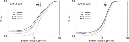
The median Einstein radius is strongly correlated with the giant-arc cross-section for the relaxed cluster subsample. Unrelaxed clusters are especially problematic for the calculation of strong lensing efficiency using the production of giant lensing arcs as a proxy; they also have smaller strong lensing efficiencies.
There exists a scaling relation between strong lensing efficiencies and mass, particularly for higher overdensities (Δ = 2500). As we move to lower overdensities, the normalization for the each simulation differs primarily due to the redistribution of baryons near the cluster core.
We search for an explanation for these findings by analysing the mass profiles of our cluster sample; the distribution of mass in the centres of clusters is significantly influenced by baryonic physics. AGN feedback reduces the stellar mass in the core of otherwise ‘overcooled’ clusters. Nevertheless, within r/Rvir ≲ 0.03 the total mass is still significantly larger than that of the DM counterparts. However, this does not translate to higher lensing efficiencies for zs =2 because θE ≳ 0.03Rvir for most clusters in our chosen mass range.
Where there is overlap in cluster masses and redshifts, our results are similar to those obtained by Duffy et al. () and Mead et al. () with regards to the effect of AGN feedback on density profiles and giant-arc cross-sections. The AGN feedback prescription used in each work is all inspired by the model of SMH but with somewhat different implementations and choice of the relevant model parameters. Therefore, it is reassuring that the strong lensing predictions are not sensitive to these details. However, Teyssier et al. (), who include thermal AGN feedback into a Eulerian AMR code, have noted that stellar fractions are sensitive to implementation. An open question is then whether different implementations of AGN feedback in different codes produce comparable effects on the inner density profiles of massive haloes and, therefore, on the strong lensing properties of galaxy clusters.
As for the comparison with observational data, available results on strong lensing arc statistics for samples of nearby and distant clusters have been recently carried out, for instance, by Horesh et al. (). Furthermore, the ongoing Cluster Lensing And Supernova survey with Hubble (CLASH; Postman et al. ) project, thanks to the superior sensitivity of deep Hubble Space Telescope imaging, is providing unprecedented detail in the internal mass distribution of galaxy clusters through strong lensing studies. These results represent an excellent test ground for the comparison with simulation results, like those presented in this paper. Self-consistent comparisons with data are deferred for future study, as this will require more careful selection of clusters, with a comparable mix of relaxed and unrelaxed objects in the observational and simulated samples, as well as consistent methods of measuring strong lensing properties. As Wyithe, Turner & Spergel () have shown, a reduction in the lensing efficiency due to a decreased mass concentration may be partially compensated by a higher magnification for individual images. Therefore, a comparison of giant arc counts will require not only a prediction for the strong lensing cross-section, but also the magnification of images that are potential giant arcs, in order to determine if they would be detected in flux-limited imaging; this is particularly important for images that lie near the flux limit.
Approaches to resolving the arc-statistics problem have generally involved questioning three aspects of the cosmological test: the assumed source redshift distribution, the realism of simulations, and the self-consistency in selection criteria for simulated and observed clusters. We prefer the Einstein radius as a proxy for strong lensing, since it allows one to avoid uncertainties with describing realistic source populations. None of the simulated models are tuned to reproduce all observable properties of clusters, but the AGN set of simulations is the most realistic one. Our study shows that AGN feedback is a game-changer; it is hard to explain a possible discrepancy between observed and simulated lensing efficiency by resorting to the effect of baryons. Therefore, it will be crucial to make self-consistent comparisons between simulations and observations at a range of redshifts to understand if lensing efficiency truly presents a challenge for ΛCDM.
The authors would like to thank Volker Springel for making available to us the non-public version of the gadget-3 code, and Annalisa Bonafede for her help with generating the initial conditions for the simulations. The authors would also like to thank the anonymous referee for useful comments that improved the paper, as well as Weiguang Cui, Geraint Lewis, Giuseppe Murante, Susana Planelles, Ewald Puchwein, Joop Schaye, Piero Rosati and Simon White for helpful discussions. Simulations have been carried out at the CINECA Supercomputing Centre in Bologna (Italy), with CPU time assigned through ISCRA proposals and through an agreement with University of Trieste. MK acknowledges a fellowship from the European Commission's Framework Programme 7, through the Marie Curie Initial Training Network CosmoComp (PITN-GA-2009-238356). DF acknowledges funding from the Centre of Excellence for Space Sciences and Technologies SPACE-SI, an operation partly financed by the European Union, European Regional Development Fund and Republic of Slovenia, Ministry of Higher Education, Science and Technology. This work has been supported by the PRIN-INAF09 project ‘Towards an Italian Network for Computational Cosmology’, by the PRIN-MIUR09 ‘Tracing the growth of structures in the Universe’ and by the PD51 INFN grant.
It is informative to consider AGN feedback prescriptions implemented in Adaptive Mesh Refinement (AMR) codes, such as those presented by Teyssier et al. (). They report a stellar mass fraction of f★ ≈ 0.01 which increases with resolution to f★ ≈ 0.02. Although the concept of mass resolution is not directly comparable between SPH and AMR codes, their results do caution that AGN feedback may be sensitive to resolution.
