


Abstract
Foreground removal is a major challenge for detecting the redshifted 21 cm neutral hydrogen (H i) signal from the Epoch of Reionization. We have used 150 MHz Giant Metrewave Radio Telescope observations to characterize the statistical properties of the foregrounds in four different fields of view. The measured multifrequency angular power spectrum Cℓ(Δν) is found to have values in the range 104–2 × 10⁴ mK2 across 700 ≤ ℓ ≤ 2 × 10⁴ and Δν ≤ 2.5 MHz, which is consistent with model predictions where point sources are the most dominant foreground component. The measured Cℓ(Δν) does not show a smooth Δν dependence, which poses a severe difficulty for foreground removal using polynomial fitting.
The observational data were used to assess point source subtraction. Considering the brightest source (∼1 Jy) in each field, we find that the residual artefacts are less than 1.5 per cent in the most sensitive field (FIELD I). Considering all the sources in the fields, we find that the bulk of the image is free of artefacts, the artefacts being localized to the vicinity of the brightest sources. We have used FIELD I, which has an rms noise of 1.3 mJy beam−1, to study the properties of the radio source population to a limiting flux of 9 mJy. The differential source count is well fitted with a single power law of slope −1.6. We find there is no evidence for flattening of the source counts towards lower flux densities which suggests that source population is dominated by the classical radio-loud active galactic nucleus.
The diffuse Galactic emission is revealed after the point sources are subtracted out from FIELD I. We find Cℓ ∝ ℓ−2.34 for 253 ≤ ℓ ≤ 800 which is characteristic of the Galactic synchrotron radiation measured at higher frequencies and larger angular scales. We estimate the fluctuations in the Galactic synchrotron emission to be  at ℓ = 800 (θ > 10 arcmin). The measured Cℓ is dominated by the residual point sources and artefacts at smaller angular scales where Cℓ ∼ 103 mK2 for ℓ > 800.
1 INTRODUCTION
Observations of the high-redshift Universe with the 21-cm hyperfine line emitted by neutral hydrogen gas (H i) during the Epoch of Reionization (EoR) contains a wealth of cosmological and astrophysical information (see Furlanetto, Oh & Briggs ; Morales & Wyithe , for recent reviews). Analysis of quasar absorption spectra (Becker et al. ; Fan et al. ) and the cosmic microwave background radiation (CMBR; Komatsu et al. ) together indicates that reionization probably started around a redshift of 15 and lasted until a redshift of 6. The Giant Metrewave Radio Telescope (GMRT; Swarup et al. ) is currently functioning at several bands in the frequency range of 150–1420 MHz and can potentially detect the 21-cm signal at high redshifts. Several upcoming low-frequency telescopes such as Low Frequency Array (LOFAR), Murchison Widefield Array (MWA) and Precision Array for Probing the Epoch of Reionization (PAPER) are also targeting a detection of the high-redshift 21-cm signal. LOFAR is already operational and will soon start to collect data for the EoR project.
In this paper we have carried out GMRT observations to characterize the statistical properties of the background radiation at 150 MHz. These observations cover a frequency band of ∼5 MHz with a ∼100 kHz resolution, and cover the angular scales ∼30 arcmin to ∼30 arcsec. The 21 cm radiation is expected to have an rms brightness temperature of a few mK on angular scales of a few arcminute (Zaldarriaga, Furlanetto & Hernquist ). This signal is, however, buried in the emission from other astrophysical sources which are collectively referred to as foregrounds. Foreground models (Ali, Bharadwaj & Chengalur ) predict that they are dominated by the extragalactic radio sources and the diffuse synchrotron radiation from our own Galaxy which makes a smaller contribution. Analytic estimates of the H i 21-cm signal indicate that the predicted signal decorrelates rapidly with increasing Δν and the signal falls off 90 per cent or more at Δν ≥ 0.5 MHz (Bharadwaj & Sethi ; Bharadwaj & Ali ). The foreground from different astrophysical sources is expected to be correlated over a large frequency separation. This property of the signal holds the promise of allowing us to separate the signal from the foregrounds (Ghosh et al. ). In this paper we have characterized the foreground properties across a frequency separation Δν of 2.5 MHz, the signal may be safely assumed to have decorrelated well within this frequency range.
There currently exist several surveys which cover large regions of the sky at around 150 MHz like the 3CR survey (Edge et al. ; Bennett ), the 6C survey (Hales, Baldwin & Warner ; Waldram ) and the 7C survey (Hales et al. ). These surveys have a relatively poor angular resolution and a limiting flux density of ∼100 mJy. Di Matteo et al. () have used the 6C survey, the 3CR survey and the 3CRR catalogue (Laing, Riley & Longair ) to estimate the extragalactic point source contribution at 150 MHz. The GMRT, which is currently the most sensitive telescope at 150 MHz, offers the possibility to perform deeper surveys with a higher angular resolution. A few single pointing 150 MHz surveys (Sirothia et al. ; Ishwara-Chandra et al. , ; Intema et al. ) have been performed with an rms noise of ∼1 mJy beam−1 at a resolution of 20–30 arcsec. The TIFR GMRT Sky Survey (TGSS) is currently underway to survey the sky north of the declination (Dec.) −30° with an rms noise of 7–9 mJy beam−1 at an angular resolution of 20 arcsec.
Diffuse synchrotron radiation produced by cosmic ray electrons propagating in the magnetic field of our Galaxy (Ginzburg & Syrovatskii ) is a major foreground component. This component, which is associated with our Galactic disc, is particularly strong in the plane of our Galaxy. Our target fields were selected well off the Galactic plane with b > 10° where we expect a relatively lower contribution from the Galactic synchrotron radiation.
Radio surveys at 408 MHz (Haslam et al. ), 1.42 GHz (Reich ; Reich & Reich ) and 2.326 GHz (Jonas, Baart & Nicolson ) have measured the diffuse Galactic synchrotron radiation at angular scales larger than ∼1° where it is the most dominant contribution, exceeding the point sources. Platania et al. () have analysed these observations to show that the Galactic synchrotron emission has a steep spectral index of α ≈ 2.8. The angular power spectrum Cℓ has been measured at 2.3 (Giardino et al. ) and 2.4 GHz (Giardino et al. ) where they find Cℓ ∼ ℓ−2.4 at angular multipoles ℓ < 250. Wilkinson Microwave Anisotropy Probe (WMAP) data show Cℓ ∼ ℓ−2 at ℓ ≤ 200 (Bennett et al. ) which is slightly flatter compared to the findings at lower frequencies. It is relevant to note that all of these results are restricted to angular scales greater than 43 arcmin (ℓ < 250), little is known (except Bernardi et al. discussed later) about the structure of the Galactic synchrotron radiation at the subdegree angular scales probed in this paper.
Ali et al. () have carried out GMRT observations to characterize the foregrounds on subdegree angular scales at 150 MHz. They have used the measured visibilities to directly determine the multifrequency angular power spectrum (MAPS) Cℓ(Δν) (Datta, Roy Choudhury & Bharadwaj ) which characterizes the statistical properties of the fluctuations in the background radiation jointly as a function of the angular multipole ℓ and frequency separation Δν. They find that the measured Cℓ(Δν) has a value of around 104 mK2 which is seven orders of magnitude larger than the expected H i signal. The measured Cℓ(Δν) was also found to exhibit relatively large (∼10–20 per cent) fluctuations in Δν which poses a severe problem for foreground removal. Further, it was attempted to remove the foregrounds by subtracting out all the identifiable point sources above 8 mJy. The resulting Cℓ, however, only dropped to approximately three times the original value due to residual artefacts.
Bernardi et al. () have analysed 150 MHz Westerbork Synthesis Radio Telescope (WSRT) observations near the Galactic plane ((l = 137°, b = +8°) to characterize the statistical properties of the diffuse Galactic emission (after removing the point sources) at angular multipoles ℓ < 3000 (θ > 3.6 arcmin). They find that the measured total intensity angular power spectrum shows a power-law behaviour Cℓ ∝ ℓ−2.2 for ℓ ≤ 900. They also measured the polarization angular power spectrum for which they find Cℓ ∝ ℓ−1.65 for ℓ ≤ 2700. Their observations indicate fluctuations of the order of ∼5.7 and 3.3 K on 5 arcmin angular scales for the total intensity and the polarized diffuse Galactic emission, respectively. Pen et al. () have carried out 150 MHz GMRT observations at a high Galactic latitude to place an upper limit of  on the polarized foregrounds at ℓ < 1000.
There has been a considerable amount of work towards simulating the foregrounds (Gleser, Nusser & Benson ; Jelić et al. ; Sun et al. ; Bowman, Morales & Hewitt ; Harker et al. ; Liu, Tegmark & Zaldarriaga ; Liu et al. ) in order to develop algorithms to subtract the foregrounds and detect the redshifted 21-cm signal. These simulations require guidance from observational data, and it is crucial to accurately characterize the foregrounds in order to have realistic simulations for future observations.
One of the challenges for the detection of this cosmological 21-cm signal is the accuracy of the foreground source removal. Our current paper aims at characterizing the foreground at arcminute angular scales which will be essential for extracting the 21-cm signal from the data. In this paper we study the radio source population at 150 MHz, which is still less explored, to determine the differential source count which plays a very important role in predicting the angular power spectrum of point sources (Ali et al. ; Ghosh et al. ). We find that the point sources are the most dominating foreground component at the angular scales of our analysis. The accuracy of point source removal is one of the principal challenges for the detection of the 21-cm signal. We investigate in detail the extragalactic point source contamination in our observed fields and study how accurately the bright point sources can be removed from our images. We also estimate the level of residual contamination in our images. It is expected that the diffuse Galactic emission will be revealed if the point sources are individually modelled and removed with high level of precession. To our knowledge, the present work is only the second time that the fluctuations in the Galactic diffuse emission have been detected at around 10 arcmin angular scales at a frequency of 150 MHz. We also complement this with a measurement of the angular power spectrum of the diffuse Galactic foreground emission in the ℓ range 200–800.
In this paper we have analysed GMRT observations to characterize the foregrounds in four different fields at 150 MHz which corresponds to the H i signal from z = 8.3. We note that unless otherwise stated we use the cosmological parameters (Ωm0, ΩΛ0, Ωb h2, h, ns, σ8) = (0.3, 0.7, 0.024, 0.7, 1.0, 1.0) in our analysis. We now present a brief outline of the paper. Section describes the observations and data analysis. We have used the MAPS Cℓ(Δν) to quantify the statistical properties of the background radiation in the observed fields. Section presents the technique that we have used to estimate Cℓ(Δν) directly from the measured visibilities. We show the measured Cℓ(Δν), and discuss its properties in Section . In this section we have also compared the measured Cℓ(Δν) with foreground model predictions. In Section we consider the extragalactic point sources which form the most dominant foreground component in our observations. In order to assess how well we can subtract out the point sources, we consider point source subtraction for the brightest source in each field, as well as subtracting out all the identifiable sources. We use the most sensitive field (FIELD I) in our observation to study the nature of the radio source population at 150 MHz, and we also provide a source catalogue for this field in the online version of this paper (Appendix ). In Section we have used the residual data of FIELD I, after point source removal, to study the diffuse Galactic synchrotron radiation. We have summarized the results of the entire paper in Section .
2 GMRT OBSERVATIONS AND DATA ANALYSIS
The GMRT has a hybrid configuration (Swarup et al. ), each of diameter 45 m, where 14 of the 30 antennas are randomly distributed in a central square which is approximately 1.1 × 1.1 km in extent. The rest of the antennas lie along three ∼14 km long arms in an approximately ‘Y’ configuration. The shortest antenna separation (baseline) is around 60 m including projection effects while the largest separation is around 26 km. The hybrid configuration of the GMRT gives reasonably good sensitivity to probe both compact and extended sources. Table 0001 summarizes our observations including the calibrators used for each field. For all observations, visibilities were recorded for two circular polarizations (RR and LL) with 128 frequency channels and 16 s integration time.
Observation summary
| FIELD I | FIELD II | FIELD III | FIELD IV | |
| Date | 2008 January 08 | 2010 February 07 | 2010 February 08 | 2005 June 15 |
| Working antennas | 28 | 28 | 26 | 23 |
| Central frequency | 153 MHz | 148 MHz | 148 MHz | 153 MHz |
| Channel width | 62.5 kHz | 125.0 kHz | 125.0 kHz | 62.5 kHz |
| Bandwidth | 3.75 MHz | 8.75 MHz | 10.0 MHz | 4.37 MHz |
| Total observation time | 11 h | 6 h | 6 h | 13 h |
| Flux calibrator | 3C 147 | 3C 147 | 3C 286 | 3C 48 |
| Observation time | 1.2 h | 1.75 h | 0.5 h | 2 h |
| Flux density (Perley–Taylor 99) | ∼72.5 Jy | ∼72.6 Jy | ∼33.41 Jy | ∼62.5 Jy |
| Phase calibrator | 3C 147 | 3C 147 | 1459+716 | 3C 48 |
| Observation time | – | – | 1.6 h | – |
| Flux density | – | – | ∼38.7 Jy | – |
| Target field (α, δ)2000 | (05h30m00s, | (06h00m00s, | (12h36m49s, | (1h36m48s, |
| +60°00′00′′) | +62°12′58′′) | +62°12′58′′ ) | +41°24′23′′) | |
| Galactic coordinates (l, b) | 151°.80, 13°.89 | 151°.49, 18°.12 | 125°.89, 54°.83 | 132°.00, 20°.67 |
| Sky temp. (Haslam map, 408 MHz) | ∼40 K | ∼30 K | ∼20 K | ∼30 K |
| Observation time | 9.8 h | 4.25 h | 3.9 h | 11 h |
We have observed FIELD I in GMRT Time Allocation Committee (GTAC) cycle 15 in 2008 January, whereas FIELD II and FIELD III were observed in cycle 17 during 2010 February. Our target fields were selected at high Galactic latitudes (b > 10°) which were up at night time during the GTAC cycles 15 and 17, and which contain relatively few bright sources (≥0.3 Jy) in the 1400 MHz NRAO VLA Sky Survey (NVSS). We have selected such fields where the 408 MHz Haslam map sky temperature is relatively low (in the range of 30–40 K) and there is no significant structure visible at the angular resolution (∼0°.85) of Haslam map. FIELD IV had been observed in cycle 8 (2005 June) and the 150 MHz foregrounds in this field have been analysed and published earlier (Ali et al. ). We have used the calibrated data set of Ali et al. (), the foreground characterization has, however, been redone using an improved technique (Ghosh et al. ).
The observations were largely carried out at night to minimize the radio frequency interference (RFI) from man-made sources. Further, the ionosphere is considerably more stable at night, and the scintillation due to ionospheric oscillations is expected to go down. The duration of our observations (∼4–10 h) was chosen so as to achieve a reasonably high signal-to-noise ratio, and also to have a reasonably large number of visibilities adequate for a statistical analysis of the foregrounds.
We have followed the standard procedure of interferometric observations where we observe a flux calibrator of known strength and a phase calibrator whose structure is known but whose strength varies from epoch to epoch. The flux calibrator, which is observed at the start of the observation, sets the amplitude scale of the gains and this is used to set the amplitude of the phase calibrator. Phase calibrators were chosen near the target fields, and these were observed every half an hour so as to correct for temporal variations in the system gain. We have used the observations of the phase calibrators to determine the complex gains of the antennas, and these gains were interpolated to the observations of the target fields.
The data for FIELDS I, II and III were reduced using flagcal (Prasad & Chengalur ) which is a flagging and calibration software for radio interferometric data. FIELD IV, however, was not analysed with flagcal, it was flagged manually and then calibrated using the standard task within Astronomical Image Processing Software (aips). The details of the observation, data reduction and relevant statistics for FIELD IV are discussed in Ali et al. ().
RFI is a major factor limiting the sensitivity of at low frequencies. RFIs effectively increase the system noise and corrupt the calibration solutions. It also restricts the available frequency bandwidth. The effect is particularly strong at frequencies below 0.5 GHz. flagcal identifies and removes bad visibilities by requiring that good visibilities be continuous in time and frequency, computes calibration solutions using known flux and phase calibrators and interpolates these on to the target fields (see Prasad & Chengalur for more details). The flagged and calibrated visibility data were used to make continuum images using the standard tasks in the aips.
The large field of view (FoV; θFWHM = 3°.8) of the GMRT at 150 MHz leads to considerable error if the non-coplanar nature of the GMRT antenna distribution is not taken into account. We use the three-dimensional (3D) imaging feature (Perley ) in the aips task ‘imagr’ in which the entire FoV is divided into multiple subfields (facets), each of which is imaged separately. Table 0002 contains a summary of the imaging details with all the relevant parameters which are mostly self-explanatory.
Wide field imaging summary
| FIELD I | FIELD II | FIELD III | FIELD IV | |
| Image size | 5700 × 5700 | 5500 × 5500 | 5500 × 5500 | 5500 × 5500 |
| Pixel size | 3.22 × 3.22 arcsec2 | 3.32 × 3.32 arcsec2 | 3.27 × 3.27 arcsec2 | 3.40 × 3.40 arcsec2 |
| Number of facets | 121 with 2 overlap | 109 with 2 overlap | 109 with 2 overlap | 109 with 2 overlap |
| Off-source noise | 1.3 mJy beam−1 | 2.5 mJy beam−1 | 4.5 mJy beam−1 | 1.6 mJy beam−1 |
| Peak/noise | 700 | 620 | 422 | 550 |
| Flux density (max., min.) | (905 mJy beam−1, | (1.55 Jy beam−1, | (1.9 Jy beam−1, | (900 mJy beam−1, |
| −14 mJy beam−1) | −28 mJy beam−1) | −45 mJy beam−1) | −47 mJy beam−1) | |
| Synthesized beam | 21 × 18 arcsec2, PA = 61° | 30 × 22 arcsec2, PA = −52° | 33 × 20 arcsec2, PA = 53° | 24 × 18 arcsec2, PA = 70° |
The presence of a large number of bright sources in the fields that we have observed allows us to carry out self-calibration to improve the complex gains. This reduces the errors from temporal variations in the system gain, and spatial and temporal variations in the ionospheric properties. For all the target fields, the data went through three rounds of phase self-calibration followed by one round of self-calibration for both amplitude and phase. The phase variations often occur on time-scales of as few minutes or less. The time interval for gain correction was chosen as 5, 3, 2 and 5 min for the successive self-calibration loops. In successive self-calibration loops, the gain solution converged rapidly with less than 0.1 per cent bad solutions in each loop. The final gain table was applied to all the 128 frequency channels.
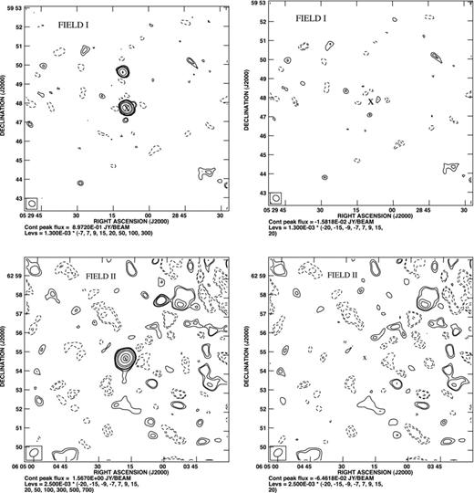
The final continuum images for the four fields are shown in Fig. 0001. The images all have a FoV of 4°.0 × 4°.0. To avoid bandwidth smearing in the continuum image, we have collapsed adjacent channels within ≤0.7 MHz and separately combined the respective images.
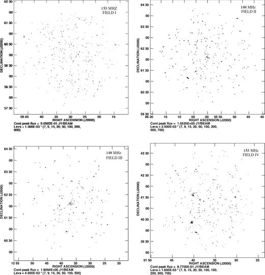
The continuum images of bandwidth 3.75, 8.75, 10.0 and 4.37 MHz of FIELD I, FIELD II, FIELD III and FIELD IV, respectively. The off source rms noise is around 1.3, 2.5, 4.5 and 1.6 mJy beam−1 for FIELD I, FIELD II, FIELD III and FIELD IV, respectively.
The subsequent analysis was done using the final; calibrated visibilities of the original 128 channel data. The final data contain visibilities for two circular polarizations. The visibilities from the two circular polarizations were combined ( ) for the subsequent analysis.
3 ESTIMATION OF ANGULAR POWER SPECTRUM FROM VISIBILITY CORRELATIONS
In this paper we have used the MAPS Cl(Δν) (Datta et al. ) to quantify the statistical properties of the sky signal. This jointly characterizes the dependence on angular scale ℓ−1 and frequency separation Δν. In this section we briefly present how we have estimated Cℓ(Δν) from the measured visibilities.
 may be expanded in spherical harmonics as

 and
and  to estimate Cℓ(Δν), where
  :
: 
For the sky signal which is dominated by foregrounds the measured Cℓ(Δν), for a fixed ℓ, is expected to vary smoothly with Δν and remain nearly constant over the observational bandwidth. In a recent 610 MHz observations (Ghosh et al. ) we find instead that in addition to a component that exhibits a smooth Δν dependence, the measured Cℓ(Δν) also has a component that oscillates as a function of Δν (around 1–4 per cent). We note that similar oscillations, with considerably larger amplitudes, have been reported in earlier GMRT observations at 153 MHz (Ali et al. ). In our recent work (Ghosh et al. ) we have noted that these oscillations could arise from bright continuum sources located at large angular separations from the phase centre. The problem can be mitigated by tapering the array's sky response with a frequency-independent window function  that falls off before the first null of the primary beam (PB). RFI sources, which are mostly located on the ground, are picked up through the side lobes of the primary beam. Tapering the array's sky response is also expected to mitigate the RFI contribution.
Close to the phase centre, the 150 MHz GMRT PB is reasonably well modelled by a Gaussian  , where the parameter θ0 is related to the full width at half-maximum (FWHM) of the PB as θ0 ≈ 0.6 θFWHM, and θ0 = 2°.3 (θFWHM = 3°.8). We taper the array's sky response by convolving the observed visibilities with a suitably chosen function
  . The sky response of the convolved visibilities
  is modulated by the window function
  which is the Fourier transform of
  . We have used a window function
  with θw < θ0 to taper the sky response so that it falls off well before the first null. We parametrize θw as θw = fθ0 with f ≤ 1, where θ0 here refers to the value at the fixed frequency 150 MHz.

 which corresponds to half of the FWHM of
  , and we have estimated
  at every grid point using all the baselines within a disc of radius 2ΔUg centred on that grid point. Using equation , however, introduces an undesirable positive noise bias in the estimated
  (e.g. Begum, Chengalur & Bhardwaj ). It is possible to avoid the noise bias if we use the estimator
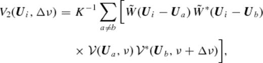
 is a normalization constant and Ua, Ub refer to the different baselines in the observational data. The noise bias is avoided by dropping the self-correlations (i.e. the terms with a = b). We finally determine Cℓ(Δν) using (Ali et al. )
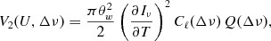
 and
and  as constants in our analysis. We have used Q(Δν) = 1 which introduces an extra Δν dependence in the estimated Cℓ(Δν). This, we assume, will be a small effect and can be accounted for during foreground removal. The gridded data have been binned assuming that the signal is statistically isotropic in U. We finally invert equation to determine the angular power spectrum:
The measured V2(U, Δν) will, in general, have a real and imaginary parts (e.g. Fig. 0002). The expectation value of V2(U, Δν) (equation ) is predicted to be real, and the imaginary part is predicted to be zero. We use the real part of the measured V2(U, Δν) to estimate Cℓ(Δν) using equation . A small imaginary part, however, arises due to the noise in the individual visibilities. The fact that we are correlating two slightly different visibilities also makes a small contribution to the imaginary part. Fig. 0002 shows the real and imaginary parts of the measured V2(U, Δν = 0) as a function of U for all the four fields that we have analysed. As expected, the imaginary part is much smaller than the real part. We use the requirement that the imaginary part of V2(U, Δν) should be small compared to the real part as a consistency check of our analysis. It also establishes that we are truly measuring a sky signal, and our results are not dominated by noise or other local effects in the individual visibilities.
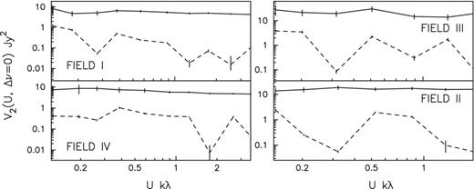
The real (upper curve) and imaginary (lower curve) parts of the observed visibility correlation V2(U, 0) as a function of baselines U. The 1σ error bars shown on the plot include contribution from both cosmic variance and system noise.
We next investigate whether tapering the sky response of the PB actually mitigates the oscillations reported in earlier work at 150 MHz (Ali et al. , FIELD IV of this paper). For this purpose, we introduce the dimensionless decorrelation function κℓ(Δν) = Cℓ(Δν)/Cℓ(0) which has the maximum value κℓ(Δν) = 1 at Δν = 0, and is in the range ∣κℓ(Δν)∣ ≤ 1 for other values of Δν. We use κℓ(Δν) to quantify the Δν dependence of Cℓ(Δν) at a fixed value of ℓ. Fig. 0003 shows κℓ(Δν) for FIELD IV with and without the tapering. We have considered f = 0.6 and 0.8 which, respectively, correspond to a tapered sky response with FWHM 2°.3 and 3°.04 as compared to the untapered PB which has a FWHM of 3°.8 at 150 MHz. The oscillatory pattern is distinctly visible when the tapering is not applied. For most values of ℓ, the oscillations are considerably reduced and are nearly absent when tapering is applied. We do not, however, notice any particular qualitative trend with varying f. The tapering, which has been implemented through a convolution, is expected to be most effective in a situation where the uv plane is densely sampled by the baseline distribution. Our results are limited by the patchy uv coverage of the observational data that is being analysed here. This also possibly explains why some small oscillations persist even after tapering is applied.
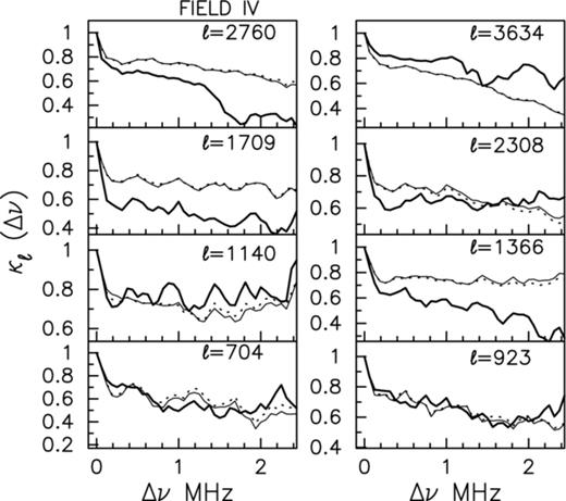
The measured κℓ(Δν) as a function of Δν for the different ℓ values as shown in each panel, for FIELD IV. The thick solid, thin solid and dotted curves show results for no tapering, and tapering with f = 0.8 and 0.6, respectively.
The results for the other fields are very similar to FIELD IV, and we have not shown these here. We have used a tapered PB with f = 0.8 for all the fields in the entire subsequent analysis.
4 THE MEASURED MAPS ![graphic]()
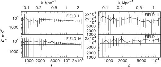
Fig. 0004 shows the measured Cℓ(Δν) and 1σ error estimates for two of our observed fields that we have analysed. We note that the 1σ error estimate has two different contributions, the cosmic variance and system noise, added in quadrature. In our observations the error is mainly dominated by the cosmic variance due to the limited number of independent estimates. The system noise makes a smaller contribution. We have determined Cℓ(Δν) in the range 0 ≤ Δν ≤ 2.5 MHz and 700 ≤ ℓ ≤ 2 × 10⁴ for FIELDS I and IV. FIELDS II and III have been observed for shorter time period (Table 0001), and the measured Cℓ(Δν) becomes relatively noisy at the large baselines which are sparsely sampled in our observational data. The ℓ range has been restricted to 700 ≤ ℓ ≤ 104 for FIELDS II and III. This corresponds to the angular scales 64 arcsec to 15 arcmin.
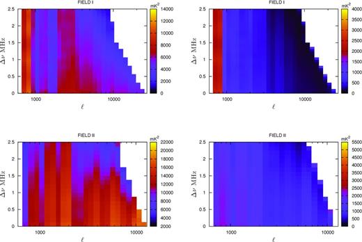
The left- and right-hand panels show the measured Cℓ(Δν) and the 1σ error bars, respectively. The white regions have been blanked as no data points are available.
A visual inspection of Fig. 0004 shows certain regions (large ℓ and Δν) where we do not have estimates of Cℓ(Δν), and these regions have been blanked in the figure. This arises due to a combination of two factors. To start with, the large baselines are sparsely sampled in the observational data. Subsequent flagging of the bad channels further depletes the data. These two factors together lead to a situation where there is practically no data at large Δν separations in the large baselines. It is reassuring to note that this effect is very similar in all the four FIELDS, of which one was manually flagged and the rest underwent automated flagging. This establishes that this effect is not an artefact introduced by the flagging technique.
Continuing with the visual inspection of Fig. 0004, we do not find any significant pattern in the variation of Cℓ(Δν) with either ℓ or Δν. However, the values seem to change more along ℓ as compared to Δν. For each of the four fields, the values of Cℓ(Δν) are nearly all within ±5σ of the mean value of Cℓ(Δν) which is 5146, 9117, 14 000 and 4939 mK2 for FIELDS I, II, III and IV, respectively. The corresponding values of σ are shown in the right-hand side of each panel of Fig. 0004. The measured Cℓ(Δν) is dominated by the contribution from extragalactic point sources, and for each field the mean value of Cℓ(Δν) is determined by the flux density of the brightest source (Sc) in that field. The variation in the mean value of Cℓ(Δν) across the different fields is primarily due to the variation in maximum source flux density Sc which has values Sc = 0.905, 1.55, 1.9 and 0.9 Jy in FIELDS I, II, III and IV, respectively (Table 0001).
We next fix Δν and study the ℓ dependence of Cℓ ≡ Cℓ(Δν = 0) (Fig. 0005). The variations in the values of Cℓ do not seem to exhibit any particular pattern, and Cℓ appears to fluctuate randomly around the mean values quoted earlier. These fluctuations, as noted earlier, are nearly all within ±5σ of the mean values (Fig. 0005). We see that the ℓ dependence of the measured Cℓ is consistent with random fluctuations arising from the statistical uncertainties in the measured Cℓ. Note that the 5σ error bars shown in Fig. 0005 reflect the estimated uncertainties arising from both, the cosmic variance and the system noise.
This shows the measured Cℓ as a function of ℓ. The constant straight line shows the mean Cℓ corresponding to each field. The range of Fourier modes k corresponding to the ℓ modes probed by our observations is also shown on the top x-axis of the figure. The 5σ error bars shown here have contributions from both the cosmic variance and system noise.
We model the measured Cℓ using the foreground model presented in Ali et al. (). The model predictions, shown in Fig. 0006, are dominated by the contribution from extragalactic point sources. At small ℓ, or large angular scales, the signal is dominated by the angular clustering of the extragalactic point sources, whereas the Poisson fluctuation due to the discrete nature of these sources is the dominant contribution at large ℓ which corresponds to small angular scales. This transition between these two occurs somewhere in the ℓ range 5000–104, and it is different in the four fields. The transition shifts to smaller ℓ values in the fields which have a larger value of Sc. The uncertainty in the model predictions is dominated by the Poisson fluctuation of the discrete point sources, and this is nearly constant across the entire ℓ range. The measured Cℓ is consistent with the predictions of the foreground model. Nearly all the measured Cℓ values lie within the 1σ error bars of the model predictions. Other astrophysical sources like the diffuse synchrotron radiation from our own Galaxy, the free–free emissions from our Galaxy and external galaxies (Shaver et al. ) make much smaller contributions, though each of these is individually larger than the H i signal.
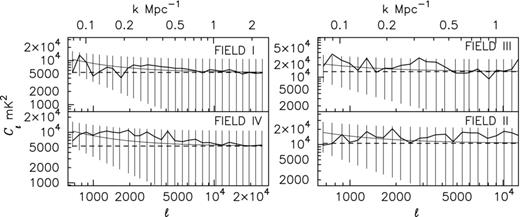
The thick solid line shows the measured Cℓ as a function of ℓ. The thin solid line with 1σ error bars shows the total foreground contribution based on the model prediction of Ali et al. (). The dashed line shows the contribution from the Poisson fluctuation of the point sources which is the most dominant contribution at large ℓ.
Both simulations (Jelić et al. ) and analytical predictions (Zaldarriaga et al. ; Bharadwaj & Ali ; Cooray & Furlanetto ; Santos et al. ) suggest that at low ℓ (ℓ ∼ 103) the EoR H i signal is approximately  , while at the larger ℓ values (ℓ ∼ 104)
  drops to 10−5–10−6 mK2. We find that the measured Cℓ, arising from foregrounds, has values around 104 mK2 at ℓ ∼ 1000, and it drops by 50 per cent at the smallest angular scales probed by our observations (ℓ ∼ 104). This suggests that the expected H i signal
  is (∼107) times smaller than the measured Cℓ arising from foregrounds.
We next shift our attention to the Δν dependence of the measured Cℓ(Δν), holding ℓ fixed. We have restricted our analysis to large angular scales (ℓ < 2000) where the H i signal is predicted to be relatively stronger, and we have a higher chance of an initial detection. We find that for nearly all the ℓ values for FIELD I and IV the variation in Cℓ(Δν) with Δν is roughly between 4 × 10³ and 104 mK2, whereas for FIELD II and III Cℓ(Δν) roughly varies between 6 × 10³ and 3.5 × 10⁴ mK2 across the 2.5 MHz Δν range that we have analysed. The fractional variation in Cℓ(Δν) ranges from ∼20 to 40 per cent for all the fields. Our foreground model prediction shows that the measured 150 MHz sky signal is dominated by extragalactic point sources. These are believed to have slowly varying, power-law να frequency spectra. We expect the resultant Cℓ(Δν) to have a smooth Δν dependence, and essentially show very little variation over the small Δν range (2.5 MHz) that we have considered here (Δν/ν ≪ 1). For a fixed ℓ, the cosmic variance is expected to introduce the same error (independent of Δν) across the entire band. As a consequence we do not show the cosmic variance for the Δν dependence of the measured Cℓ(Δν).
The measured Cℓ(Δν) is, by and large, found to decrease with increasing Δν if we hold ℓ fixed. However, contrary to our expectations, the Δν dependence is not completely smooth. There are a few ℓ values, particularly in FIELDS II and III, where the Δν dependence appears to be rather smooth. We however have abrupt variations and oscillations in the Δν dependence for most of the remaining data. FIELDS I and IV, which have a channel width of 62.5 KHz, have a relatively high frequency resolution as compared to FIELDS II and III which have a channel width of 125 KHz. For FIELDS I and IV, an oscillatory pattern is clearly visible in Cℓ(Δν) at nearly all the ℓ values. These oscillations, however, are not noticeable in FIELDS II and III which have a lower frequency resolution. It is possible that the oscillations are actually also present in FIELDS II and III, but we are missing them due to the lower frequency resolution in these two fields. To test this we have also analysed FIELDS I and IV at a lower frequency resolution by collapsing the original data. We find that the oscillations seen in FIELDS I and IV are somewhat reduced, but they can still be made out at the lower frequency resolution of 125 KHz. We find that though the oscillations in all the fields have reduced considerably after tapering the sky response (Section ), a residual oscillatory pattern still persist. The oscillations are most pronounced at the lowest ℓ values where the period of oscillation varies between ∼1 and 2 MHz (Fig. 0007). The period and amplitude of these oscillations both decrease with increasing ℓ (Fig. 0008). The exact cause of this residual oscillatory pattern is, at the moment, not known. We recollect that the sky tapering is implemented through a convolution whose efficiency depends on the uv coverage of the baselines. It is possible that the residual oscillations are a consequence of the finite and sparse uv coverage of our data.
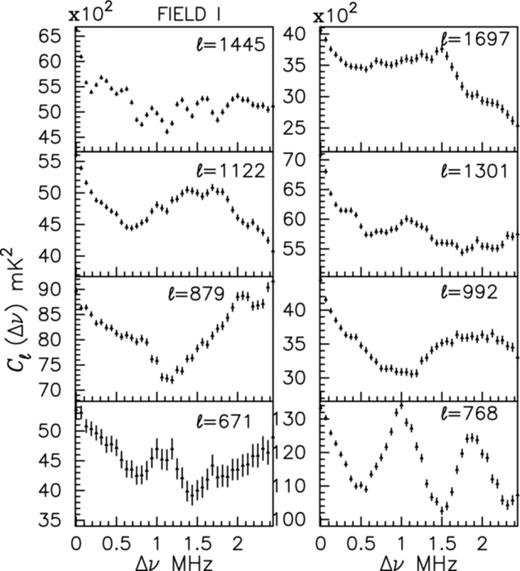
For FIELD I, this shows the measured Cℓ(Δν) as a function of Δν for the fixed values of ℓ shown in the panels. The error bars show 10σ system noise.
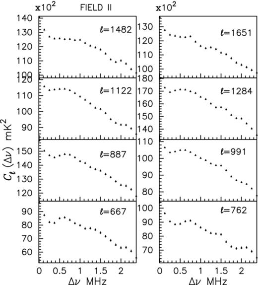
For FIELD II, this shows the measured Cℓ(Δν) as a function of Δν for the fixed values of ℓ shown in the panels. The error bars show 10σ system noise.
The oscillations and abrupt changes in the Δν dependence of Cℓ(Δν) pose a severe impediment for foreground removal. Foreground removal relies on the key assumption that the foregrounds have a Δν dependence which is distinctly different from that of the H i signal. The foreground contributions are expected to vary slowly with increasing Δν, whereas the H i signal is expected to decorrelate rapidly well within Δν ≤ 0.5 MHz (Bharadwaj & Sethi ; Bharadwaj & Ali ; Ghosh et al. ). It is then possible to remove the foregrounds by modelling and subtracting out any component that varies slowly with increasing Δν. For example, it is possible to use low-order polynomials to model the Δν dependence of the measured Cℓ(Δν) at fixed valued of ℓ, and use these to subtract out the foreground contribution (Ghosh et al. ). It is quite evident that the oscillations and abrupt changes in the Δν dependence of the measured Cℓ(Δν) pose a severe challenge for this technique, or any other technique that is based on the assumption that the foregrounds vary smoothly with frequency. It is relevant to note that Jelić et al. () and Harker et al. () have shown that the foreground subtraction using polynomial fitting can easily cause overfitting, in which we fit away some of the cosmological signal, or underfitting, in which the residuals of the foreground emission can overwhelm the cosmological signal. Therefore, one needs to use non-parametric methods that allow data to determinate their shape without selecting any a priori functional form of the foregrounds (Harker et al. ; Chapman et al. ).
We would like to point out that a possible line of approach in foreground removal is to represent the sky signal as an image cube where in addition to the two angular coordinates on the sky we have the frequency as the third dimension (Jelić et al. ; Harker et al. ; Chapman et al. ; Zaroubi et al. ). For each angular position, polynomial fitting is used to subtract out the component of the sky signal that varies slowly with frequency. The residual sky signal is expected to contain only the H i signal and noise (Jelić et al. ; Bowman et al. ; Harker et al. , ; Liu et al. ). Liu et al. () showed that this method of foreground removal has problems which could be particularly severe at large baselines if the uv sampling is sparse. We would also like to point out that in a typical GMRT observation the uv plane is not completely sampled and due to this limited baseline coverage there exist correlated noise in the image plane which is a problem for estimating the power spectrum in the image plane (for details see Dutta , appendix A). Although, the upcoming low-frequency radio telescopes such as the LOFAR, MWA, etc. will have a much dense uv coverage compared to GMRT, where in the core region most of the baselines relevant for the EoR experiments will be sampled and the foreground removal technique in image-frequency space can also be applied (Jelić et al. ; Harker et al. ; Chapman et al. ; Zaroubi et al. ).
5 POINT SOURCES
The discrete sources seen in Fig. 0001 dominate the 150 MHz radio sky at the angular scales probed in our observations. These sources are typically smaller than the angular resolution of our observations. It is now well accepted that these are extragalactic, being mainly associated with active galactic nuclei (AGN). It is of considerable interest to study the properties of these sources (Dunlop & Peacock ; Jackson & Wall ; Peacock ; Seymour, McHardy & Gunn ; Garn et al. ).
There currently exist several radio surveys at 150 MHz like the 3CR survey (Bennett ), the 3CRR catalogue (Laing et al. ), the 6C (Hales et al. ; Waldram ) and the 7C survey (Hales et al. ), which cover large regions of the sky. The 6C and 7C surveys have angular resolutions of ∼4.2 arcmin and ∼70 arcsec, respectively, and the limiting source flux density of these surveys is ∼100 mJy.
Point sources are the most dominant foreground component and it creates a major problem for detecting the 21-cm signal from the redshifted H i emission in the ℓ range 103–104 probed here. Di Matteo et al. () have used the results of the previous surveys to estimate the point source contribution to the foregrounds at 150 MHz. However, these have a limiting source flux density of ∼100 mJy, and the extrapolation to fainter sources is rather uncertain. The GMRT has an angular resolution of ∼20 arcsec at 150 MHz. We are able to achieve an rms noise of around 1.3 mJy beam−1 in the observations reported here. The GMRT is currently the only instrument capable of achieving this level of sensitivity in terms of angular resolution and rms noise. We note that there are relatively few GMRT results regarding the radio source population at 150 MHz (Intema et al. ; Ishwara-Chandra et al. ) with sensitivity comparable to that reached in our observation. Recent simulations (Bowman et al. ; Liu et al. ) also indicate that point sources should be subtracted down to a ∼10–100 mJy threshold in order to detect the EoR signal. In this section we use our 150 MHz observations to explore the population of radio sources in our observed fields down to the detection limit of ∼9 mJy.
In order to detect the H i signal, it is very important to correctly identify the point sources and subtract these out at a high level of precision (Bernardi et al. ; Pindor et al. ). It is quite evident that a template of detected point sources above a given threshold level is an essential part of foreground removal where we have noticed that the Poisson and clustering component of the point sources are the most dominating foreground component at our angular scales of analysis. We first focus on the brightest source in each of the four fields that we have analysed. In each field, the brightest source (Table 0002) alone contributes around 10 per cent of the total measured Cℓ. We consider the brightest source as a test case to investigate how well it is possible to image and subtract out the point sources.
We note that FIELDS I and IV have a relatively longer on-source observation time in comparison to FIELDS II and III, and this is reflected in the fact that FIELDS I and IV have a lower noise level and higher sensitivity in comparison to FIELDS II and III (Table 0002). The left-hand panel of Fig. 0009 shows a more detailed view of the brightest source for the most sensitive and the least sensitive fields among the four fields that we have imaged. For making these images, we have applied the appropriate phase shifts so as to bring the brightest source to the phase centre of the image. The ratio of the peak flux density to the rms noise (peak/noise, Table 0002) has a maximum value of 700 in FIELD I, and a minimum value of (422) in FIELD III. The brightest source in each of our fields is also found to be accompanied by several regions of negative flux density. These are presumably the result of residual phase errors which were not corrected in our self-calibration process. We find that the peak negative flux density is 14 mJy beam−1 in FIELD I, and 47 mJy beam−1 in FIELD IV. These correspond to 1.5 and 5.3 per cent of the peak flux density in the respective fields, the values lie within this range for the two other fields (Table 0002). In addition to the pixels with negative flux densities, we also see several regions of positive flux densities well above the 5σ noise levels. Both the positive and negative regions are imaging artefacts which are possibly the outcome of calibration errors. The self-calibration steps implemented in the earlier stage of the analysis have considerably reduced the imaging artefacts. The artefacts, however, not entirely removed through self-calibration. A visual inspection of the image of the brightest source in FIELD I (top left-hand panel of Fig. 0009) shows that there are around 10 distinct features with flux densities around 7 mJy arising from imaging artefacts. The artefacts effectively increase the local rms noise in the vicinity of the brightest source, and reduce the dynamic range of the image.
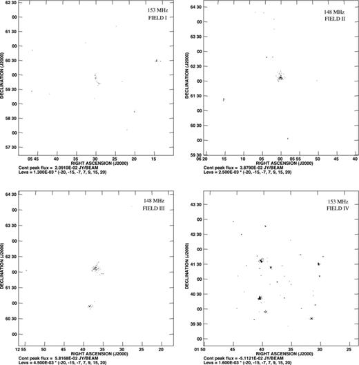
The position around the brightest source (marked with ‘X’) for FIELDS I and II before (left-hand panel) and after (right-hand panel) the source is subtracted.
We next consider how well we can subtract out the brightest source in the four fields that we have analysed. We model the brightest source using the clean components of the continuum image. The visibilities corresponding to these clean components were subtracted from the original full frequency resolution uv data using the aips task uvsub. The right-hand panel of Fig. 0009 shows the continuum image made with the residual visibilities after the brightest source was subtracted out. We find that the peak residual has values (−15, −64, −54, 34) mJy beam−1 which correspond to (1.6, 4.0, 3.1, 3.8) per cent of the original source that was subtracted out from the four fields, respectively. FIELD I has the least residuals and the image is largely featureless in comparison to FIELD II which has the maximum residuals.
The continuum image used for source subtraction does not take into account the possibility that the variation in the source flux across the observational band. In principle, we do not expect a significant flux variation across the relatively small frequency bands in our observation. Fig. 0010 shows the channel spectra through the brightest pixel in two of our observed fields. Contrary to our expectation, we find 15–30 per cent variations in the spectra. Further, these variations are not smooth and they show random and abrupt variations. The channels where data are missing have been flagged to avoid broad-band RFI. This spectral variation is mainly due to errors in the bandpass calibration. It is very clear that it will not be very effective to model the observed spectral variation of the source using a smooth polynomial or power law. It may be a better strategy to make separate images at each frequency channel and individually subtract out the clean component from each channel of the uv data, provided the signal-to-noise ratio is sufficient for single channel images.
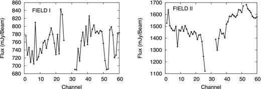
The flux/beam versus channel (frequency) plots at the brightest source position for two fields. Note that some channels were heavily corrupted by broad-band RFIs and we flagged those channels which are shown as ‘gap’ in FIELDS I and II.
We next consider source subtraction from the entire FoV. Pixels with flux density above 7σ times the rms noise were visually identified as sources and subtracted out using exactly the same procedure as used for the brightest source. It is expected that at this stage most of the genuine sources seen in Fig. 0001 have been removed from the uv data. Fig. 0011 shows the corresponding images made from the residual visibilities after source subtraction. The flux density in these images is in the range of (21, 39, 58, 30) to (−14, −29, −51, −51) mJy beam−1, respectively, for the four fields that we have analysed. Most of the residuals, we find, are clustered in a few regions in the image. These regions have a typical angular extent of 15 arcmin and are centred on the locations of the bright sources in the FoV. The residuals are essentially imaging artefacts that were not modelled using clean components. The rest of the image, leaving aside a few isolated regions, is largely free of artefacts and devoid of any visible feature. We find that FIELD I has the highest sensitivity (lowest rms noise) amongst our observed fields. We also see that source removal is most effective for this field. We see (Fig. 0011) that most of the image is free of residual structures after source subtraction, except for two small regions where most of the artefacts are localized. It is quite evident that FIELD I is the best field and we use this for the entire subsequent analysis.
The same as Fig. 0001 except that all the pixels with flux density above 7σ noise value were visually identified as genuine sources and not artefacts have been fitted with clean components and removed from the visibility data from which this image was made. It is expected that most of the genuine sources have been removed from this data.
5.1 Differential source count
The differential source count plays a very important role in estimating the power spectrum of point sources. Further, this also provides invaluable information as to the nature of the radio sources. Here we evaluate the differential source count using the discrete sources identified in FIELD I down to a flux limit of 9 mJy.
We use the aips task sad to identify and extract the sources from the continuum image of FIELD I (Fig. 0001). sad identifies potential sources based on the peak brightness and fits a Gaussian model to the sources. Source identification was restricted within a radius of 1°.45 from the phase centre, where the primary beam response is within 50 per cent of its central value. We have used a conservative peak brightness detection limit of 7σ (>9 mJy beam−1) for the initial source selection using sad. This minimizes the number of noise spikes that are spuriously detected as sources.
As mentioned earlier, the local rms noise increases near the bright sources due to the presence of imaging artefacts. We have estimated the local rms in different parts of the residual image by applying the aips task rmsd. The local rms at each pixel was estimated using an area of approximately 256 × 256 pixels centred on that pixel. Sources with a peak brightness in excess of 5σ times the local rms noise were finally selected. Further, we have visually inspected the regions close to the brightest sources and discarded sources that appeared to be imaging artefacts. This ensures that we do not include any bright imaging artefacts as sources. The flux density of all the extracted sources was corrected for the GMRT primary beam using an eighth-order polynomial (Kantharia & Pramesh Rao ).
We have finally identified a total of 206 sources (Fig. 0012) within a 1°.45 radius from the pointing centre. The full source catalogue is given in the online version of the paper (Appendix ) and is presented in order of increasing right ascension (RA). For each source, the catalogue lists the position of the sources in RA, Dec., peak flux density, local rms noise at the source location, the integrated flux density and the error in the integrated flux density.
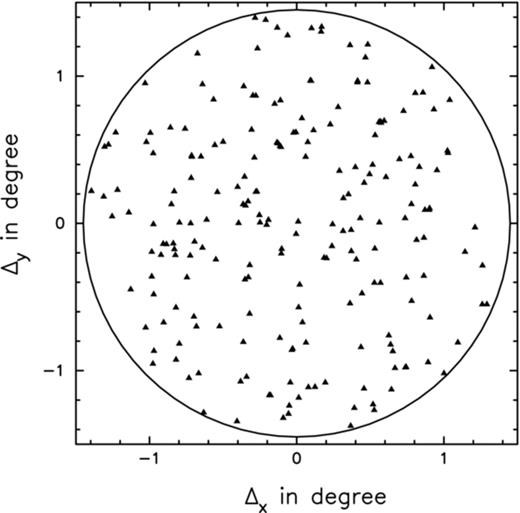
The triangles show the 206 sources within a radius of 1°.45 from the phase centre. Here, Δx = cos (Dec.C)(RA − RAC) and Δy = (Dec. − Dec.C) are the angular displacements from the phase centre RAC and Dec.C. The RA and Dec. represent the positions of the different sources.
We have used the source catalogue to determine the differential source count dN/dS, the number of sources dN in the flux interval dS. Note that S here refers to the integrated flux density of the source. To determine dN/dS we have binned the sources in the range 9.11 ≤ S ≤ 945.71 mJy into 10 logarithmic bins in S (Table 0003) and counted the number of sources (N) in each bin. We next consider two corrections that have to be considered in interpreting the source counts. The first is the Eddington bias where the random noise artificially boosts the number of sources in the faintest bin. The 7σ detection limit and the subsequent visual inspection help to avoid spurious sources and minimize the effect of the Eddington bias. Further, studies at 610 MHz, Moss et al. () indicate that the Eddington bias only influences the faintest flux density bin, increasing the source count by approximately 20 per cent. Since the number of sources in our lowest flux bin is comparatively small, we decided to make no correction for this effect.
150 MHz differential source counts for FIELD I. The columns show bin flux limits, the mean flux density of sources in each bin, number of sources, the noise corrected number of sources and dN/dS with error
| Flux bin | S | N | Nc | dNc/dS |
| (mJy) | (mJy) | (sr−1 Jy−1) | ||
| 9.11–14.49 | 12.23 | 9 | 32.82 | (3.03 ± 0.53) × 106 |
| 14.49–23.06 | 18.48 | 25 | 35.15 | (2.04 ± 0.34) × 106 |
| 23.06–36.68 | 29.38 | 44 | 44.16 | (1.61 ± 0.24) × 106 |
| 36.68–58.35 | 44.96 | 38 | 38.00 | (8.72 ± 1.41) × 105 |
| 58.35–92.82 | 72.71 | 27 | 27.00 | (3.89 ± 0.75) × 105 |
| 92.82–147.67 | 118.51 | 23 | 23.00 | (2.08 ± 0.43) × 105 |
| 147.67–234.91 | 192.87 | 18 | 18.00 | (1.03 ± 0.24) × 105 |
| 234.91–373.70 | 306.16 | 10 | 10.00 | (3.58 ± 1.13) × 104 |
| 373.70–594.48 | 495.95 | 8 | 8.00 | (1.80 ± 0.64) × 104 |
| 594.48–945.71 | 799.70 | 4 | 4.00 | (5.66 ± 2.83) × 103 |
The second effect is related with the fact that extended sources with peak brightnesses below the survey limit but integrated flux densities above this limit would not be detected by our source detection procedure. It is possible to get an estimate of this effect with the knowledge of the angular size distribution of the sources as a function of flux density. This helps to identify the incompleteness due to extended sources in the estimated source count distribution, well known as resolution bias. Recently, Moss et al. () have estimated that they will miss approximately 3 per cent of the sources due to the resolution bias at 610 MHz. In our case, we do not find a significant number of extended sources and therefore we choose to make no correction for this effect.

 to estimate the error in the differential source count.
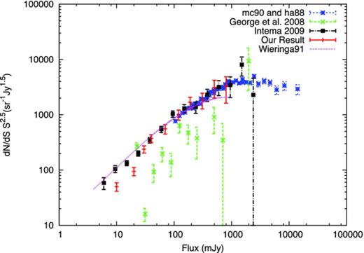
The differential source counts at 150 MHz (mc90 and ha88: McGilchrist et al. and Hales et al. ; George & Stevens ; Intema et al. ; our result), normalized by the value expected in a static Euclidean universe. A steady decrease in the source counts is observed as we approach lower flux values. The continuous curve represents the functional form of the fit (valid from 4 mJy to 1 Jy) to the source counts by Wieringa (), scaled down to 150 MHz assuming a mean spectral index of −0.70.
This source count model was scaled down to our observing frequency of 150 MHz assuming that the source fluxes can be scaled as S ∝ ν−α. We have tried out various values of the mean spectral index α. We find that the model (equation ) is most consistent with our measurements for a mean spectral index of α = 0.7 (Fig. 0013).
We find that our differential source count (Fig. 0013) which is determined over a flux range from 9 mJy to 1 Jy is well fitted by a single power law of slope 0.97 ± 0.07. We note that George & Stevens () have estimated a single power law of slope 0.72 in the flux range of 20 mJy to 2 Jy from a 150 MHz GMRT survey centred around ε Eridanus. In Fig. 0013 we show the normalized differential source count from their survey. We find that they have underdetermined the normalized differential source count in the entire flux range and it is most likely due to the low number of sources (113) that were used to determine the source count. For comparison we also plot the combined results from 6C and 7C surveys in Fig. 0013. We find that there is a good agreement between our source count and those derived from the 6C and 7C surveys (Hales et al. ; McGilchrist et al. ) in the flux range 0.1–1.0 Jy. Intema et al. () have determined the normalized differential source count at 153 MHz using a catalogue of 598 sources in the flux range of 4.75 mJy to 3 Jy. We notice that our source counts are roughly equal to their in the high flux range of 30.0 mJy to 1.0 Jy. Towards the lower flux ends (<30.0 mJy) we find their source counts are increasingly higher compared to our source count. We note that our estimated source count agrees well with Ishwara-Chandra et al. () in the low flux range (<30.0 mJy) where they found a relatively low population of sources compared to Intema et al. ().
The simulated source count model proposed by Jackson () at 151 MHz predicts a flattening in the power-law shape below 10 mJy due to a growing population of Fanaroff–Riley (Fanaroff & Riley ) class I (FR I) radio galaxies. The turnover in the source count is a well-known observed feature at 1.4 GHz (Condon ; Hopkins et al. ; Seymour et al. ) and occurs around 1 mJy, which is equivalent to ∼5 mJy for an average spectral index of 0.7. We note that although this flattening is observed in deep radio surveys at higher frequencies (1.4 GHz: Windhorst, Mathis & Neuschaefer ; 610 MHz: Garn et al. , ), our current survey depth is not sufficient to detect this flattening. This suggests that our catalogue is dominated by the classical radio-loud AGN population which are the predominant sources at higher flux densities.
We note that the predicted angular power spectrum Cℓ (Fig. 0006) does not change very significantly if we use the differential source count measured here instead of the foreground model used for the predictions in Section .
6 DIFFUSE GALACTIC FOREGROUND
The diffuse synchrotron radiation from our Galaxy dominates the sky at low radio frequencies like 150 MHz. Haslam et al. () surveyed the full sky with an angular resolution of 0°.85 at 408 MHz using single dish observations. The sky brightness temperature is found to vary in the range 11–4247 K across the entire sky. Assuming that the synchrotron brightness temperature scales as T ∝ ν−2.8 with frequency (Platania et al. ), we have a conversion factor of 16.47 from 408 to 150 MHz. This gives the brightness temperature range from 181 to 69 948 K across the entire sky at 150 MHz, and (660, 495, 330, 495) K at the respective phases centres of the four fields that we have observed (Table 0001). The subsequent analysis is restricted to FIELD I where we have been able to achieve the best sensitivity, and point source subtraction is also most effective. Further this is the lowest Galactic latitude field (b = 13°.89) among our observed fields and it may provide an upper limit on the expected diffuse foreground emission for four fields that we have observed. Fig. 0014 shows the 408 MHz (Haslam et al. ) brightness temperature distribution within a 10° × 10° region of FIELD I. The figure also shows the 150 MHz brightness temperature distribution obtained by scaling the 408 MHz maps. The scaling to 150 MHz takes into the angular variation of the spectral index (Platania et al. ), and we have used LFmap (Polisensky ) to generate the data for these figures. The smallest baseline in our observation is around U = 100, which corresponds to an angular scale of U−1 ≈ 30 arcmin. Our observations are not sensitive to intensity variations at angular scales larger than this, and consequently we do not expect the structures seen in Fig. 0014 to be imprinted in our observation. Very little is known about the angular structure of the diffuse Galactic synchrotron radiation on subdegree scales.
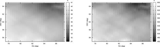
In the left-hand panel we show the brightness temperature distribution around FIELD I at 408 MHz (Haslam et al. ) after destriping (Platania et al. ). In the right-hand panel we show the temperature values at 150 MHz where we scale the temperature values with the average spectral index map from Platania et al. (). We use Polisensky () to generate this figures.
Model predictions (Ali et al. ), which extrapolate the statistical properties measured at large angular scales and higher frequencies, predict that point sources are the most dominant contribution at subdegree scales. We expect the diffuse radiation to dominate if the point sources can be individually modelled and removed with high level of precession. Bernardi et al. () have analysed 150 MHz WSRT observations where they have subtracted out the point sources to reveal the structure of the fluctuations in the diffuse Galactic synchrotron radiation at 13 arcmin angular scales. We note that their observation was carried out at a low Galactic latitude (b = 8°) where the Galactic emission is expected to be relatively larger than our targeted field. It is expected that we should be able to use the residual data to characterize the diffuse radiation provided the point sources have been removed to an adequate level of sensitivity.
We have discussed point source subtraction in Section . For FIELD I, Figs 0001 and 0011 show 4°.0 × 4°.0 continuum images of the field before and after source subtraction. All the pixels with flux density greater than 10 mJy beam−1 were visually inspected, and those which appeared to be genuine sources were fitted with clean components using tight boxes. The continuum clean components were then subtracted from the visibility data. The image, after source subtraction, has residual flux density in the range of −14 to 21 mJy beam−1 arising from imaging artefacts. We recollect here that these residuals are highly localized in the vicinity of a few regions that contained the brightest sources (Fig. 0011). The bulk of the field is largely free of artefacts and is consistent with noise.
It is possible that very bright sources beyond the 4°.0 × 4°.0 field that we have imaged also contribute to the measured visibilities. To account for this possibility we have also imaged a 8°.0 × 8°.0 region after the sources within the central 4°.0 × 4°.0 region have been subtracted out. We have then removed all the sources automatically to a 10 mJy beam−1 level using the 8°.0 × 8°.0 image.
We expect to see the diffuse background radiation after the point sources have been removed, however, the high-resolution (20 × 18 arcsec2) residual image does not exhibit any diffuse structure. The noise and the residuals after point source removal appear to dominate the high-resolution image. We expect the Galactic synchrotron radiation to be relatively larger in comparison to the noise and residuals if we consider larger angular scales. We have considered the angular scale 10 arcmin, and following Bernardi et al. () we have made two images which refer to this angular scale. Initially, we made an image which does not have any visibilities with baselines |U | < 170. This restriction imposes the condition that the resulting image does not contain any information on angular scales greater than 10 arcmin. For the second image (Fig. 0015), the visibilities were tapered with a Gaussian in the uv plane so as to produce a synthesized beam of FWHM 620 × 540 arcsec2. This image does not contain information at angular scales below 10 arcmin.
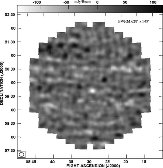
The image where we tapered the uv plane at |U | = 200. The synthesized beam has a FWHM of 620 × 540 arcsec2. All the genuine point sources were removed down to 10 mJy level. Diffuse structures begin to appear on >10 arcmin scales. The brightest structures in this map are at a ∼5σ level compared to the local rms of 23.5 mJy beam−1.
We see that the image, made by including only the baselines |U | > 170, which does not contain any information above 10 arcmin looks very similar to the high-resolution image. Both of these images are dominated by the noise, and the residuals from the brightest point sources are seen to be localized near the centre of the image. In contrast, the low-resolution image (Fig. 0015), which does not contain information at angular scales below 10 arcmin, shows fluctuations which are uncorrelated with the point source distribution seen in the high-resolution image (Fig. 0001). The maximum and minimum values of flux density in Fig. 0015 are 113 and −139 mJy beam−1, respectively, which are comparable to 5σ, where σ (rms) is 23.5 mJy beam−1 (Table 0004). The individual regions corresponding to the very high (or low) pixel values also have an angular extent that is comparable to the synthesized beam. We interpret these features, which correspond to brightness temperature fluctuations of the order of 20 K (Table 0004), as a tentative detection of the Galactic synchrotron radiation at the 10 arcmin angular scale.
Rms fluctuations in the FIELD I as a function of angular resolution
| Angular | Rms | Conversion factor | Rms |
| resolution | (mJy beam−1) | (mJy beam−1) to (K) | (K) |
| 20 × 18 arcsec2 | 1.30 | 171.80 | 223.34 |
| 620 × 540 arcsec2 | 23.50 | 0.17 | 4.00 |
| 1070 × 864 arcsec2 | 35.00 | 0.06 | 2.1 |
| Angular | Rms | Conversion factor | Rms |
| resolution | (mJy beam−1) | (mJy beam−1) to (K) | (K) |
| 20 × 18 arcsec2 | 1.30 | 171.80 | 223.34 |
| 620 × 540 arcsec2 | 23.50 | 0.17 | 4.00 |
| 1070 × 864 arcsec2 | 35.00 | 0.06 | 2.1 |
We next increase the uv taper to produce a synthesized beam with a larger FWHM of 1070 × 864 arcsec2. Fig. 0016 shows the corresponding image which does not have any information at angular scales below approximately 16 arcmin. The maximum and minimum values of flux density in this image are 436 and −353 mJy beam−1, respectively, which are greater than 10σ, where σ (rms) is 35 mJy beam−1 (Table 0004). The individual regions corresponding to the very high (or low) pixel values have an angular extent that is comparable to, if not bigger than, the synthesized beam. In fact the size of these regions approaches the largest angular scales (∼30 arcmin) that can be probed in our observation. We interpret these 10σ fluctuations as a detection of the fluctuations in the Galactic synchrotron radiation at the 16 arcmin angular scale. Converting to brightness temperature (Table 0004), we have a peak fluctuation of 26 K in our FoV.
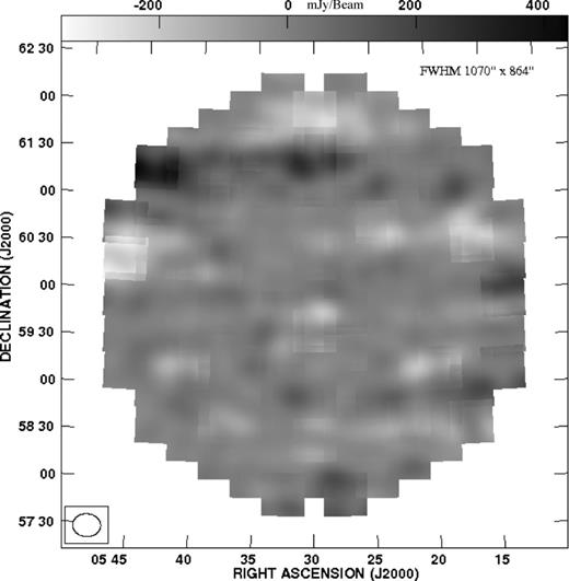
The image where we tapered the uv plane at |U | = 100. The synthesized beam has a FWHM of 1070 × 864 arcsec2. All the genuine point sources were removed down to 10 mJy level. The brightest structures in this map are at a 10σ level compared to the local rms of 35 mJy beam−1.
Based on our observation we conclude that the residuals after point source subtraction represent structures in the Galactic synchrotron radiation on angular scales of 10–20 arcmin. The noise and the residuals from point source subtraction, however, dominate the data at smaller angular scales where we are unable to make out the Galactic synchrotron radiation.
6.1 Power spectrum
We have used the visibilities, after point source subtraction, to estimate the angular power spectrum Cℓ ≡ Cℓ(Δν = 0). The angular power spectrum Cℓ (Fig. 0017) clearly shows two different scaling behaviour as a function of ℓ. At low angular multipoles (ℓ ≤ 800), which correspond to angular scales larger than 10 arcmin, we find a steep power-law behaviour which is typical of the Galactic synchrotron emission observed at higher frequencies and larger angular scales (Bennett et al. ). The angular power spectrum flattens out for l > 800, and we find that it remains nearly flat out to ℓ ≈ 8000 which corresponds to angular scales of ∼1 arcmin. The nearly flat region arises from the point sources which have a flux that is below the threshold for source identification and removal, and hence have not been subtracted from the data. The errors in modelling and subtracting the identified sources also contribute to this.
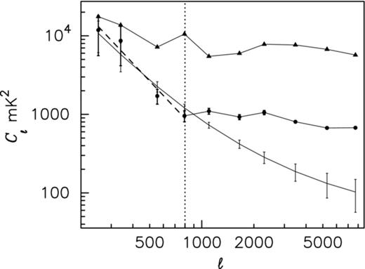
The measured Cℓ before (triangle) and after (circle) source subtraction, with 1σ error bars shown only for the latter. The dashed line shows the best-fitting power law (ℓ ≤ 800) after source removal. The thin solid line (lowest curve) with 1σ error bars shows the model prediction of Ali et al. () assuming that all point sources above Sc = 20 mJy have been removed.
 at ℓ = 800 which is comparable to the 20 K features seen in the 10 arcmin resolution image (Fig. 0015). We have used a weighted least square to fit a power law,
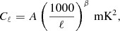
Bernardi et al. () have analysed 150 MHz WSRT observations, where they have subtracted out point sources above 15 mJy and used the resulting image to estimate the angular power spectrum Cℓ. We note that their analysis differs from our in that they have estimated Cℓ from the image whereas we have directly used the measured visibilities to estimate Cℓ (Fig. 0017). Our findings, however, are very similar to those of Bernardi et al. () who find that the measured Cℓ is well described by a power law for ℓ ≤ 900. Their best-fitting parameters are A = 253 ± 40 mK2 and β = 2.2 ± 0.3. The slope, we note, is consistent with our findings, the amplitude, however, is half to our value. The difference in amplitude is not surprising as the two different values refer to observations in two different parts of the sky. The amplitude measured by Bernardi et al. () refers to a field with Galactic latitude b = 8°, whereas FIELD I of our observations is at b = 13°.89. We would generally expect lesser synchrotron emission in our field which is at a higher elevation from the Galactic plane, however, the amplitude of Cℓ shows the opposite behaviour. The variation of the subdegree scale angular structure of the Galactic synchrotron emission across different parts of the sky is not known at present, and it is not possible to make any conclusive statement about this apparent discrepancy. It is possible that there may be some extra power coming from the clustering of unresolved point sources below ℓ ≤ 800. We note that our estimate of the angular power spectrum for the Galactic diffuse emission (Fig. 0017) matches quite well with the foreground model prediction of Ali et al. (), assuming that all point sources above a threshold flux limit of 20 mJy (see for reference top left-hand panel of Fig. 0011, FIELD I) have been removed.
Strictly speaking, it is not justified to compare the amplitude of the angular power spectrum obtained in observations at two different frequencies unless their slopes (angular spectral index) are consistent with each other. We have not found any other observations (except Bernardi et al. ) of the northern Galactic plane where the angular spectral index is consistent with our findings. Despite this, we have used an earlier work (La Porta et al. ) at higher frequencies to estimate the amplitude of the angular power spectrum expected at our observing frequency. La Porta et al. () have estimated angular power spectrum of all-sky total intensity maps at 408 (Haslam et al. ) and 1420 MHz (Reich ; Reich & Reich ; Reich, Testori & Reich ). The angular power spectrum of the Galactic synchrotron emission is measured down to the angular mode of ℓ = 200 and 300 at 408 and 1420 MHz, respectively. Using the best-fitting parameters (tabulated at ℓ = 100) at 408 and 1420 MHz, we obtain the amplitude of the angular power spectrum Cℓ = 200 ≃ 230 and 0.22 mK2, respectively, close to the Galactic latitude of b = 15° (close to FIELD I). By extrapolating the values of Cℓ = 200 from 408 and 1420 MHz using a mean frequency spectral index of α = 2.5 (de Oliveira-Costa et al. ) (Cℓ ∝ ν−2 α) we find that the expected contributions at 150 MHz from the Galactic synchrotron emission are 3.42 × 10⁴ and 2.08 × 10⁴ mK2, respectively. In our observation we find Cℓ = 200 = 2.22 × 10⁴ mK2 which lies within the range 2.08 × 10⁴–3.42 × 10⁴ mK2, and hence we conclude that our finding is consistent with the values extrapolated from higher frequency and larger angular scales.
Giardino et al. () have analysed the fluctuations in the Galactic synchrotron radiation using the 2.3 GHz Rhodes Survey where they find a slope β = 2.43 ± 0.01 across the range 2 ≤ ℓ ≤ 100. Giardino et al. () have analysed the 2.4 GHz Parkes radio continuum and polarization survey of the southern Galactic plane where they find a slope β = 2.37 ± 0.21 across the range 40 ≤ ℓ ≤ 250. Our slope, measured at smaller angular scales, is consistent with these findings. There has been considerable work on modelling the Galactic synchrotron radiation at the higher frequencies relevant for the CMBR (tens of GHz). These models predict a power-law scaling behaviour Cℓ ∝ ℓ−β, where β have values in the range 2.4–3 down to ℓ = 900 (Tegmark & Efstathiou ; Tegmark et al. ).
We note that the slope measured by us at 150 MHz is consistent with these model predictions. Bennett et al. () have determined the angular power spectrum of the Galactic synchrotron radiation using the WMAP data in the frequency range 23–94 GHz. Their measurement is restricted to ℓ ≤ 200 where they find a scaling Cℓ ∼ ℓ−2 which is slightly flatter than the slope we obtain at smaller angular scales.
7 DISCUSSION AND CONCLUSIONS
We have analysed 150 MHz GMRT observations in four different fields of view (Table 0001, Fig. 0001). We have used the MAPS Cℓ(Δν) to jointly characterize the statistical properties of the fluctuations as a function of the angular multipole ℓ and the frequency separation Δν (Fig. 0004) across the range 700 ≤ ℓ ≤ 2 × 10⁴ and 0 ≤ Δν ≤ 2.5 MHz. We find that the measured Cℓ has values around 104 mK2 at ℓ ∼ 1000, and it drops by around 50 per cent at ℓ ∼ 104. The measured Cℓ is foreground dominated and is more than seven orders of magnitude larger than the expected H i signal.
Analytic estimates of the H i signal (Bharadwaj & Ali ) show that we expect  to decorrelate rapidly with increasing Δν, and fall by 90 per cent or more at Δν ≥ 0.5 MHz. In contrast, the foregrounds from different astrophysical sources are expected to be correlated over large frequency separations (Δν > 2 MHz). This holds the promise of allowing us to separate the signal from the foregrounds (Ghosh et al. ). We find that the measured Cℓ(Δν) (for reference see Figs 0007 and 0008) shows a smooth Δν dependence with a 20–40 per cent variation across the measured 2.5 MHz Δν range. However, contrary to our expectations, in addition to a smooth behaviour we also notice abrupt variations and oscillations (≤10 per cent) in the Δν dependence of the measured Cℓ(Δν). These abrupt variations and oscillations, whose origin is at present not understood, pose a severe impediment for foreground removal. Polynomial fitting along the frequency axis has been extensively considered for foreground removal. All attempts in this direction may fail due to the presence of abrupt variations and small oscillations which cannot be filtered out with low-order polynomials.
The measured Cℓs, we find, are consistent with foreground models which predict that extragalactic point sources make the most dominant contribution at the subdegree scales that we have probed here (Fig. 0006). The brightest source (∼1 Jy) in each field alone contributes around 10 per cent of the total measured Cℓ. It is very important to correctly identify the point sources and subtract these out at a high level of precision. We have carried out point source subtraction in all the four fields that we have analysed here (Figs 0009 and 0011). Considering only the brightest source, we find that source subtraction is most effective in FIELD I, where the image also has the lowest rms noise of 1.3 mJy beam−1 (Table 0002). The residual artefacts after subtracting out the brightest source, we find, are within 1.5 per cent of the of the original source flux (905 mJy).
The subsequent analysis was restricted to FIELD I which has the lowest rms noise. The clean components corresponding to all the sources above 10 mJy were subtracted out from the visibility data using the aips task uvsub. We find that the resulting angular power spectrum Cℓ falls to ∼1000 mK2 in the ℓ range 800–8000 (Fig. 0017), which is roughly one-tenth of the Cℓ before source subtraction. At these multipoles, we interpret the measured Cℓ, after source subtraction, as arising from a combination of the residual artefacts from the bright sources and the faint sources (<10 mJy) that have not been removed. The behaviour at lower multipoles (ℓ ≤ 800), we find, is well fitted by a power law Cℓ = (513 ± 41) × (1000/ℓ)2.34 ± 0.28 mK2 which we interpret as the contribution from the diffuse Galactic synchrotron radiation. The measured slope is consistent with earlier WSRT 150 MHz observations (Bernardi et al. ), and also with 2.3 and 2.4 GHz results at smaller ℓ (Giardino et al. , ), whereas WMAP finds a flatter slope Cℓ ∼ ℓ−2 (Bennett et al. ) at smaller ℓ and much higher frequencies (23–94 GHz).
AG would like to thank M. H. Wieringa for sharing the third chapter of his thesis. AG thanks Emil Polisensky for a detailed discussion on LFmap. AG acknowledges CSIR, India, for providing financial support through Senior Research Fellowship (SRF). SSA acknowledges the support by DST, India, under Project No. SR/FTP/PS-088/2010. We thank Heinz Andernach of Depto. de Astronomia, Mexico regarding the presentation of source catalogue. The data used in this paper were obtained using GMRT. The GMRT is run by the National Centre for Radio Astrophysics of the Tata Institute of Fundamental Research. We thank the GMRT staff for making these observations possible.
REFERENCES
Appendix A
SOURCE CATALOGUE
The complete 150 MHz GMRT source catalogue, listed in ascending order of right ascension. This is a sample of the full table, which is available as Supporting Information with the online version of the paper
| Source name | RA | Dec. | Peak | Local noise | Int. flux density | Error |
| (J2000.0) | (J2000.0) | (mJy beam−1) | (mJy beam−1) | (mJy) | (mJy) | |
| GMRT J051850.9+601311.6 | 05:18:50.91 | +60:13:11.6 | 43.74 | 2.28 | 66.22 | 5.92 |
| GMRT J051931.0+601053 | 05:19:30.96 | +60:10:53.0 | 37.39 | 2.04 | 38.08 | 4.22 |
| GMRT J051933.8+603114 | 05:19:33.75 | +60:31:14.4 | 31.42 | 2.38 | 37.90 | 4.31 |
| GMRT J051946.6+603205 | 05:19:46.62 | +60:32:05.3 | 125.07 | 2.34 | 206.97 | 6.11 |
| GMRT J051958.5+600249 | 05:19:58.52 | +60:02:49.9 | 18.84 | 1.91 | 19.08 | 3.68 |
| GMRT J052010.1+603703.0 | 05:20:10.06 | +60:37:03.0 | 25.16 | 2.22 | 29.63 | 4.86 |
| GMRT J052016.0+601339 | 05:20:16.04 | +60:13:39.5 | 31.43 | 1.92 | 42.68 | 4.61 |
| GMRT J052052.9+600426 | 05:20:52.94 | +60:04:26.4 | 108.84 | 1.86 | 128.28 | 3.87 |
| GMRT J052059.2+593306 | 05:20:59.24 | +59:33:06.4 | 23.36 | 2.02 | 37.92 | 5.07 |
| GMRT J052146.0+605705 | 05:21:46.01 | +60:57:05.9 | 47.74 | 2.14 | 68.69 | 5.69 |
