Comparison of star formation rates from Hα and infrared luminosity as seen by Herschel^⋆ Free

Abstract

1 Introduction

The star formation rate (SFR) is one of the most important parameters to study galaxy evolution, as it accounts for the number of stars being formed in a galaxy per unit time. Many authors have studied the evolution of the SFR density with time, showing that the peak of the star formation took place at z ∼ 1–2, then slowing down at later times [see the data collection from different surveys by Hopkins & Beacom (2006) and recent Herschel results from Gruppioni et al. (2010)]. There is also agreement in the fact that SFR directly correlates with the galaxy properties such as gas content, morphology or mass. Recent papers such as Elbaz et al. (2011), Wuyts et al. (2011b), Daddi et al. (2010), Rodighiero et al. (2010) or Noeske (2009) have investigated in detail the existence of a main sequence in the SFR–mass relation. Therefore, it is fundamental to have a rigorous way to measure SFR when studying galaxy evolution.

A great effort has been made over the past years to derive SFR indicators from luminosities at different wavelengths, spanning from the UV, where the recently formed massive stars emit the bulk of their energy, to the infrared, where the dust-reprocessed light from those stars emerges, to the radio, which traces supernova activity, to the X-ray luminosity, tracing X-ray binary emission (e.g. Kennicutt 1998, hereafter K98; Yun, Reddy & Condon 2011; Kewley et al. 2002; Ranalli et al. 2003; Calzetti et al. 2005, 2007, 2010; Schmitt et al. 2006; Alonso-Herrero et al. 2006; Rosa-González et al. 2007; Calzetti & Kennicutt 2009). Recent works combine optical and infrared observations to derive attenuation-corrected Hα and UV continuum luminosities of galaxies by combining these fluxes with various components of IR tracers (e.g. Gordon et al. 2000; Inoue 2011; Hirashita et al. 2001; Bell et al. 2003; Hirashita, Buat & Inoue 2003; Iglesias-Páramo et al. 2006; Cortese et al. 2008; Kennicutt et al. 2009; Wuyts et al. 2011a).

The SFR derived from the Hα emission line is calibrated on the physical basis of photoionization. The nebular lines effectively re-emit the integrated stellar luminosity of galaxies shortwards the Lyman limit, so they provide a direct, sensitive probe of the young massive population. Only stars with masses >10 M_⊙ and lifetimes <20 Myr contribute significantly to the integrated ionizing flux, so the emission lines provide a nearly instantaneous measure of the SFR, independent of the previous star formation history. However, a large part of the light emitted by young stars, which mostly reside within or behind clouds of gas and dust, is absorbed by dust and then re-emitted at longer wavelengths. To properly calculate the SFR from Hα emission line an extinction correction must be applied to take this effect into account.

The absorbed light from these young stars, tracers of the SFR, is re-emitted at IR wavelengths. Therefore, the SFR can also be derived from the IR emission of the galaxies. One of the most commonly used methods to derive the SFR from the IR emission is to apply the K98 relation, which links the SFR to the IR luminosity (L_IR). However, this is a theoretical relation based on the starburst synthesis models of Leitherer & Heckman (1995) obtained for a continuous burst, solar abundances and a Salpeter (1955) initial mass function (IMF), assuming that young stars dominate the radiation field throughout the UV-visible and that the far-infrared (FIR) luminosity measures the bolometric luminosity of the starburst. This physical situation holds in dense circumnuclear starbursts that power many IR-luminous galaxies. In the disc of normal galaxies or early-type galaxies, the situation is much more complex as dust heating from the radiation field of older stars may be very important. Strictly speaking, as remarked by K98, the relation above applies only to starburst with ages less than 10⁸ years while, for other cases, it would be probably better to rely on an empirical calibration of SFR/L_IR.

The advent of the Herschel Space Telescope, which samples the critical FIR peak of nearby galaxies, is an excellent opportunity to empirically derive the relation between the observed L_IR and the SFR without associated uncertainties due to extrapolation of the IR peak. In this paper we analyse a FIR (100 or 160 μm) selected sample in the COSMOS field with associated multi-band photometry and 20k zCOSMOS optical spectroscopy at z = 0.1–0.46. We determine the SFR estimates from the Hα line luminosity corrected for extinction, while we obtain the L_IR by integrating from eight to 1000 μm the best-fitting SED of our galaxies. We test if the SFR derived from the Hα emission and the SFR derived from the L_IR are consistent at different redshifts and physical properties of the galaxies [mass, metallicity, SSFR or morphological type].

This paper is organized as follows. Section 2 introduces our sample of galaxies. Sections 3 and 4 explain the method used to derive the fundamental physical parameters of our sample (L_IR, stellar masses, SFR from dust extinction corrected Hα emission line). Section 5 presents the comparison of the two SFR indicators, while in Section 6 we discuss the effect of different galaxy properties on the comparison of the two SFR estimates. Finally, in Section 7 we summarize our conclusions.

Throughout this paper we use a standard cosmology (Ω_m = 0.3, Ω^Λ = 0.7), with H₀ = 70 km s⁻¹ Mpc⁻¹. The stellar masses are given in units of solar masses (M_⊙), and both the SFRs and the stellar masses assume a Salpeter IMF.

2 Data

We study the SFR derived from the L_IR making use of the recent Herschel data in the COSMOS field. The Herschel data include Photodetector Array Camera and Spectrometer (PACS; Poglitsch et al. 2010) data from the PEP survey (PACS Evolutionary Probe; Lutz et al. 2011). We use the PACS blind catalogue v2.1 (containing 7313 sources) down to 3σ, corresponding to ∼5 and 10.2 mJy at 100 and 160 μm, respectively. This catalogue was associated using the likelihood ratio technique (Sutherland & Saunders 1992) to the deep 24 μm catalogue from Le Floch et al. (private communication S_lim(24 μm) = 80 μJy; Sanders et al. 2007; Le Floc'h et al. 2009) and to the multi-band 3.6 μm selected catalogue from Ilbert et al. (2010) [S_lim(3.6 μm) = 1.2 μJy], including NUV, u*, B_J, g⁺, V_J, r⁺, i⁺, z⁺, J, K_s, 3.6, 4.5, 5.8, 8.0 and 24 μm from GALEX, Subaru, Infrared Array Camera (IRAC) and Spitzer legacy surveys, respectively. We also need the spectroscopic information to accurately measure the SFR from the Hα emission line. We have 1654 sources (∼23 per cent of PEP catalogue) with spectroscopic information from the zCOSMOS 20k spectroscopic survey (Lilly et al. 2009), 717 of them with z < 0.46. This cut in redshift is necessary to properly observe the Hα emission line (6562.8 Å). We did not consider sources with no accurate redshifts (flag z ≤ 2.1; Lilly et al. 2009, ∼5 per cent), neither sources with signal-to-noise ratio (S/N) < 3 in the Hα flux (∼25 per cent). We did not consider galaxies with very high values of aperture correction (>16; four galaxies) to exclude significant uncertainties associated with this correction.

To avoid active galactic nuclei (AGN) contamination we have cleaned our sample of possible AGN candidates. Type-1 AGNs are easily recognizable by their broad permitted emission lines and have been excluded originally from the zCOSMOS galaxy sample. We have eliminated sources classified as Seyfert 2 or LINERs (Low Ionization Nuclear Emission Line Region) using the Balwin–Phillips–Terlevich (BPT) diagnostic diagrams from Bongiorno et al. (2010), as well as XMM–Newton (Hasinger et al. 2007) and Chandra detected sources (Elvis et al. 2009). We have also performed an SED fitting from the NUV to the PEP bands to our sources using the Polletta et al. (2007) templates which include different SEDs, from elliptical and spiral normal galaxies, to starburst, composite, Seyfert 1 and Seyfert 2. We also used the modified templates by Gruppioni et al. (2010), which include a higher IR bump to better fit the observed FIR data. We have carefully inspected the resulting SED fits and have eliminated those sources with a typical SED of a Seyfert. This procedure allows us to identify AGN sources which could be missed by the other methods (e.g. galaxies with too low S/N to be used in the BPT diagrams). We identify 47 AGN candidates (∼6 per cent) and eliminate them. The final sample consists of 474 PEP detected Hα-emitting galaxies with 0.06 < z < 0.46. In Table 1 we summarize some of the main statistical properties of our sample (z, stellar mass, SFR, SSFR, metallicity and Hα, Hβ equivalent widths).¹

Table 1.

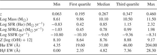
Properties of the 474 sample galaxies, indicated by their minimum and maximum value, as well as the median, the first and the third quartile

Open in new tabDownload slide

3 Sed Fitting: Infrared Luminosities and Masses

3.1 Infrared luminosities

To derive the L_IR value of each source we have performed an SED fitting using the le phare code (Arnouts et al. 2001; Ilbert et al. 2006), which separately fits the stellar part of the spectrum with a stellar library and the IR part (from 7 μm) with IR libraries. To perform the SED fitting we used four different infrared libraries (Dale et al. 2001; Chary & Elbaz 2001 and Lagache cold and Lagache SB from Lagache et al. 2004) and set them as a free parameter, i.e. for each source, the code chooses the best-fitting template of all the four libraries. This helps producing more accurate fitting to the data than choosing only one IR library. The code first performs a template-fitting procedure based on a simple χ² minimization; then it integrates the resulting best-fitting spectra from eight to 1000 μm and directly gives as an output the L_IR value. We fixed the redshift to the spectroscopic redshift (z_s) of each source and made use of multi-wavelength data, including IRAC, Spitzer 24 μm and recent PEP Herschel data at 100 and 160 μm. The inclusion of these new data at large wavelengths, which sample the critical FIR peak of nearby galaxies, allows us to derive the L_IR without associated uncertainties due to extrapolation of the IR peak (see Elbaz et al. 2010; Nordon et al. 2012). We estimate the 1σ uncertainty of the L_IR as half the difference between L_{IR, sup} and L_{IR, inf}, where L_{IR, sup} and L_{IR, inf} are the L_IR values for Δχ² = 1. In Fig. 1 we show some examples of our SED fittings. Black circles are the observed data, while the best SED fitting are the blue and the red lines for the stellar and starburst component, respectively. Notice the importance of the PEP data at 100 and 160 μm to accurately sample the IR peak of the spectra emission.

Figure 1.

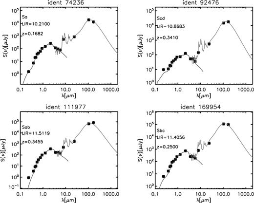
Example of SED fitting for four sources. The observed SED of each source (black filled circles) is shown with the corresponding best-fitting solution (blue solid line for the stellar part, and red solid line for the IR), as well as the morphological type (see Section 6.6), the z_s and the derived L_IR.

Open in new tabDownload slide

3.2 Stellar masses

The galaxy stellar masses have been derived as explained in Domínguez Sánchez et al. (2011) (see also Ilbert et al. 2010). We have used the le phare code to fit our multi-wavelength data (from NUV to 5.8 μm) with a set of SED templates from Maraston (2005) with star formation histories exponentially declining with time as SFR ∝ e^−t/τ. We used nine different values of τ (0.1, 0.3, 1.0, 2.0, 3.0, 5.0, 10.0, 15.0 and 30.0 Gyr) with 221 steps in age. The metallicity assumed is solar. Dust extinction from SED fitting was applied to each galaxy using the Calzetti et al. (2000) extinction law. In this paper we allow a maximum E(B − V) value of 1.4. This value was chosen as the highest E(B − V) that the code was able to handle, given the large grid of parameters used in the SED fitting, and is significantly larger than the highest E(B − V) value that we derive for our sample [E(B − V)_max = 0.85; see Section 4]. The derived age of each galaxy must be less than the age of the Universe at the redshift of that galaxy and greater than 10⁸ years (the latter requirement avoids having best-fitting SEDs with unrealistically high SSFR = SFR/M). The Maraston (2005) models include an accurate treatment of the thermally pulsing asymptotic giant branch (TP-AGB) phase, which has a high impact on modelling the templates at ages in the range 0.3 ≲ t ≲ 2 Gyr, where the fuel consumption in this phase is maximum, specially for the near-IR part; although their accurateness is still debated by a number of recent observational studies (Kriek et al. 2010; Melbourne et al. 2012).

4 SFR from Hα Emission Line

In this paper we will derive the SFR from the Hα emission line luminosity corrected for extinction [SFR(Hα) hereafter]. We will use the conversion factor derived by Kennicutt, Tamblyn & Congdon (1994) and Madau, Pozzetti & Dickinson (1998) to obtain our SFR from the Hα emission line:

1

Hα emission line fluxes were measured using the automatic routine Platefit Visible Multi Object Spectrograph (VIMOS; Lamareille et al. 2009). After removing a stellar component using Bruzual & Charlot (2003) models, Platefit VIMOS performs a simultaneous Gaussian fit of all emission lines using a Gaussian profile. The slits in the VIMOS masks have a width of 1 arcsec, therefore an aperture correction for slit losses is applied to each source. Each zCOSMOS spectrum is convolved with the Advanced Camera for Surveys (ACS) I(814) filter and then this magnitude is compared with the I-band magnitude of the GIM2D fits of Sargent et al. (2007). The difference between the two magnitudes gives the aperture correction for each spectrum. This correction assumes that the emission line fluxes and the I-band continuum suffer equal slit losses.

A major problem when deriving SFR(Hα) is the effect of dust extinction. Star formation normally takes place in dense and dusty molecular cloud regions, so a significant fraction of the emitted light from young stars is absorbed by the dust and re-emitted at IR wavelengths. A method to measure the extinction is to compare the observed ratio of the Hα and Hβ emission lines R_obs with the theoretical value (R_th = Hα/Hβ = 2.86). Then the reddening towards the nebular regions E(B − V), following Calzetti et al. (2000) extinction law, can be written as

Note that this A_V and E(B − V) values refer to the attenuation and reddening towards the nebular regions (as they are derived from the nebular emission lines), and not to the attenuation and reddening towards the stellar continuum usually found in literature and which do not necessarily take the same values (see Calzetti et al. 2000; Wuyts et al. 2011a).

Making use of the spectra of our sources from the 20k survey we can measure the observed ratio between the emission lines and obtain the extinction values. However, the quality of the spectra is not high enough to individually measure the Hβ line for the whole sample. To improve the S/N of the spectra we construct average spectra by adding spectra of galaxies with similar L_IR values. We constructed six average spectra composed of 31 galaxies each with different average L_IR values: log L_IR(L_⊙) = [9.8, 10.1, 10.4, 10.7, 11.0, 11.3].

For each average spectrum we have measured the Hα and Hβ fluxes using iraf, after subtracting the stellar component making use of more than 230 Bruzual & Charlot (2003) template models with different values of extinction. Fig. 2 shows one of the average spectra (black line) before subtracting the stellar continuum (red line) and after subtraction of the continuum (blue line). Once the stellar component is subtracted from the observed spectra, the emission lines can be measured without contamination by the stellar absorption. Fig. 3 shows the six average spectra of our sources after performing the continuum subtraction, as well as the values of the observed ratio between Hα and Hβ emission lines, A_V and E(B − V).

Figure 2.

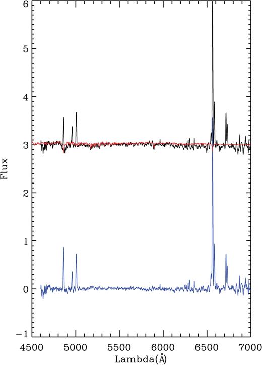
The black line represents the average spectrum for the lowest average L_IR before subtracting the stellar component (red), while the spectrum obtained when removing the stellar continuum is plotted in blue.

Open in new tabDownload slide

Figure 3.

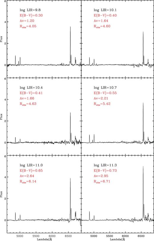
Average spectra in six L_IR bins. Also shown are the values of R_obs, A_V and E(B − V).

Open in new tabDownload slide

There is a very clear trend between the extinction and the L_IR, as can be seen in Fig. 4, where we plot the E(B − V) value derived from the average spectra with respect to the average log L_IR of each average spectrum. The relation between dust extinction and L_IR has also been previously studied by Wang & Heckman (1996), where the authors conclude that the Hβ/Hα ratio decreases with L_IR (meaning that the dust extinction increases with L_IR, in agreement with Fig. 4). We fitted the data of Fig. 4 with a straight line, obtaining a relation between log L_IR and extinction of the form:

2

The data follow the derived relation with almost no scatter. We can interpolate these data and derive an E(B − V) value for each galaxy from its L_IR and correct the Hα flux of each galaxy making use of the Calzetti et al. (2000) extinction law:

3

We then derive the Hα luminosities using the measured spectroscopic redshift z_s of each source, and finally we obtain the SFR(Hα) following equation (1).

Figure 4.

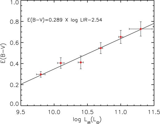
E(B − V) versus log L_IR for the six average spectra. The thick line is the best fit to the data, with a slope m = 0.29 (see equation (2)).

Open in new tabDownload slide

Our main source of SFR(Hα) error is likely to be the dust extinction correction. To test the effect of using a linear relation between the extinction and log L_IR instead of using single values of extinction derived for each galaxy, we have visually inspected the spectra of our sources and have selected a small sub-sample of 29 sources with high S/N continuum in both the Hα (S/N_c > 2) and Hβ (S/N_c > 5) spectral ranges, so that we can rely on the measured value of the Hα/Hβ ratio to derive E(B − V) for each source (R_{obs, ind}). In Fig. 5 we show the difference between the E(B − V) value obtained through the linear relation between log L_IR and E(B − V) and the E(B − V) value measured for each source for this control sample of 29 galaxies. The dispersion is σ = 0.20, with a small, not significant, offset (〈Δ(E(B − V)〉 = −0.07). This small offset confirms that, when using the linear relation between extinction and log L_IR instead of using individually measured extinctions, we are not introducing a systematic bias but only increase the dispersion of the data. We interpret the value σ = 0.20 as the E(B − V) uncertainty that we introduce in the SFR(Hα) derivation.

Figure 5.

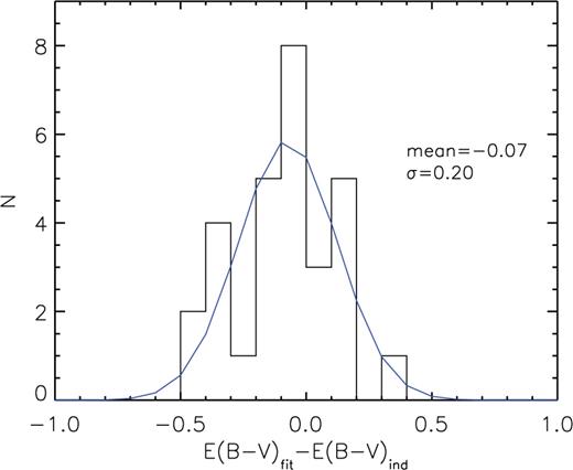
Difference between the E(B − V) value derived from the linear relation from equation (2) and the E(B − V) value measured for each source for a control sample of high S/N galaxies in the continuum both in the Hα and in Hβ spectral ranges. The Δ(E(B − V)) values are consistent with a Gaussian distribution with σ = 0.20. We assume this dispersion to be the uncertainty in E(B − V) that we introduce when using an average extinction instead of an individual extinction.

Open in new tabDownload slide

5 SFR Comparison

In this section we will compare the SFR(Hα) with the SFR derived from the L_IR. We have converted our L_IR values into SFR making use of the K98 relation, which simply multiplies the L_IR by a constant:

4

In Fig. 6 we compare the SFR(Hα) with the SFR(L_IR). The blue line is the one-to-one relation, while the red line is the best fit to our data. For the clarity of the figure we do not include the errors for each source, but show the median error on log SFR(L_IR) and log SFR(Hα) at the right hand of the plot. We have performed a linear fit taking into account the errors in both SFR(L_IR) and SFR(Hα). The latter include also the uncertainty introduced when using median extinctions (as explained in Section 4). The slope of our relation is m = 1.01 ± 0.03. Also the normalizations of the two relations are well consistent with each other with a very small offset of ∼−0.08 ± 0.03 dex. Therefore, there is an excellent agreement between the two SFR indicators. It is interesting to notice the relatively small dispersion of the data (σ = 0.28), comparable with the uncertainties derived for the SFR(Hα) (with a mean error ∼0.30). This is mainly due to the large uncertainties introduced in the SFR(Hα) derivation when using a linear relation between log L_IR and the dust extinction values instead of using the E(B − V) values for each galaxy. Considering the wide range of SFRs studied (about two orders of magnitude) and the systematic errors that could in principle affect our sample, we confirm that the two SFR estimates are in an excellent agreement, even if both of them are based on very simple recipes that do not take into account the galaxies’ intrinsic properties, but are a mere transformation from luminosity to SFR.

Figure 6.

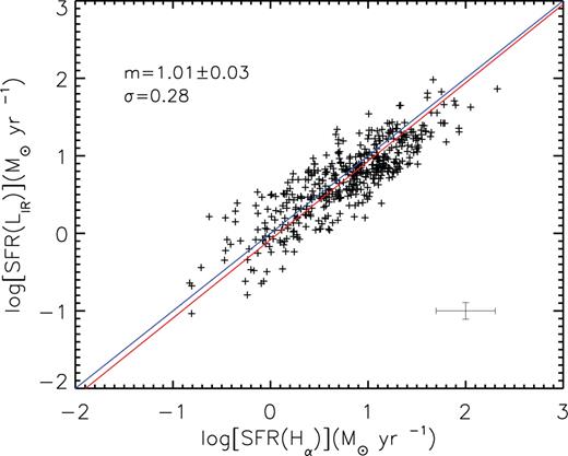
SFR(L_IR) versus SFR(Hα).The blue line represents the one-to-one relation, while the red line is the best fit to our data. Also shown in the plot is the slope of the best fit (m = 1.01 ± 0.03) and the dispersion of the relation (σ = 0.28). The median error on log SFR(L_IR) and log SFR(Hα) is shown towards the lower right of the plot.

Open in new tabDownload slide

Our results are consistent with the previous work by Kewley et al. (2002), where the authors compare SFRs from Hα luminosity and L_IR for a local sample of galaxies from the Nearby Field Galaxy Survey. After reddening correction, they derive a slope of 1.07 ± 0.03 and a normalization constant of −0.04 ± 0.02, in a very good agreement with the values that we have obtained.

It should be mentioned that, since the dust-corrected SFR(Hα) is, in the absence of measurement uncertainties, per definition, the total SFR, while the SFR(L_IR) is only the obscured part of the total, the good one-to-one correspondence between SFR(Hα) and SFR(L_IR) implies that the unobscured SFR is much lower than the obscured SFR. This is true since our sample is PEP-detected and is in agreement with the result of Caputi et al. (2008), where the authors show that the SFR forms the UV and the total SFR (IR+UV) differs by a factor of ∼10 on average for a 24 μm selected sample from the zCOSMOS-bright 10k survey. When studying a random, not IR-detected, sample of galaxies, the emission from young stars coming out unobscured in the UV may be significant, in which case the SFR(L_IR) would not be in such a good agreement with the total SFR(Hα).

We have considered the possible bias in our results which might be induced by a selection of the sample in the FIR bands. For the sources with a detected Hα flux, but not detected in the FIR, we have derived the SFR from the Hα luminosity and then transformed this into L_IR assuming that the K98 relation is correct (i.e. inverting equation (4)). There is a quite robust and well-defined correlation between L_IR and 100 and 160 μm fluxes for a given redshift. Therefore, knowing the redshift and the L_IR, we have calculated the approximate PEP fluxes that these sources should have if they would follow the K98 relation. 99 per cent of the sources detected in Hα but not detected in the FIR, have estimated PEP fluxes lower than the PEP detection limit, i.e. they are consistent with following the K98 relation and being undetected in the FIR.

We have also studied a possible aperture correction effect. The IR fluxes at 100 and 160 μm from Herschel are integrated fluxes over the whole galaxy due to the large point spread function. Instead, as explained in Section 4, the Hα is measured with a slit of 1 arcsec width and then aperture corrected. This correction assumes that the radial Hα flux distribution is the same as the radial distribution of the continuum in the I(814) ACS for each galaxy. However, we know that galaxies have internal structures, especially affecting the star-forming regions where the Hα emission line is observed. Larger galaxies should be more affected by aperture correction as the observed Hα flux is measured in a smaller part of the galaxy, while for small galaxies almost all the light enters into the slit. We have tested the aperture correction effect by comparing the difference between SFR(L_IR) and SFR(Hα) with the angular sizes of the galaxies. We did not see any systematic effect, i.e. the Δ(SFR) does not depend on the galaxy sizes. We therefore conclude that the aperture correction does not systematically affect the slope of the SFR(L_IR)–SFR(Hα) relation.

Finally, we remind that our sample misses about 25 per cent objects with PACS detection but Hα S/N < 3. These may include ‘ageing’ objects with low SSFR, extending trends discussed in Section 6.5, as well as some of the most dust obscured systems.

6 SFR(L_IR)–SFR(Hα) Relation Dependences

We have seen that both SFR estimates agree very well with each other for the sample of galaxies as a whole. In this section we aim to detect which intrinsic properties of the galaxies could affect the SFR(Hα)–SFR(L_IR) relation.

6.1 Redshift

In Fig. 7 (upper panel) we show log SFR(L_IR) versus log SFR(Hα) for different redshifts, where the colour code is explained in the plot. To better appreciate the effect of z, we plot in the lower panel the ratio between log SFR(L_IR) and log SFR(Hα) versus z. The red dots are the running mean of the Δ(SFR) = log SFR(L_IR)−log SFR(Hα) every 20 values of z. The error bar on the left hand of the plot represents the typical mean error of the running mean (σ_{rm, z} = 0.06). There seems to be no significant dependence of the relation on the redshift, but a random scatter around zero. We conclude that the SFR(L_IR)–SFR(Hα) relation is not highly affected by the redshift of the galaxies, at least up to z = 0.46, which is the maximum considered z of our sample.

Figure 7.

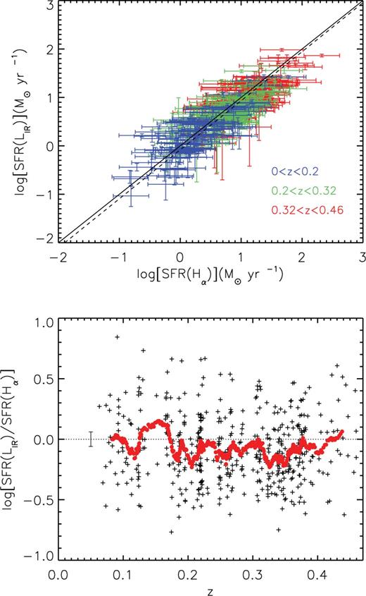
Upper panel: log SFR(L_IR) versus log SFR(Hα) for different redshift bins. Dashed and continuous lines represent the best fit to our data and the one-to-one relation, respectively. Lower panel: Δ(SFR) = log SFR(L_IR)−log SFR(Hα) versus z. Red dots are the running mean of Δ(SFR) every 20 values of z. Also shown at the left hand of the plot is the typical mean error of the running mean.

Open in new tabDownload slide

6.2 Mass

In Fig. 8 we show the ratio between log SFR(L_IR) and log SFR(Hα) versus the stellar mass. The black dots are the running mean of the Δ(SFR) = log SFR(L_IR)−log SFR(Hα) every 20 values of mass and the error bar on the left hand of the plot represents the typical mean error of the running mean (σ_{rm, M} = 0.06). In this case, there is not only a random scatter around zero, but there is also a slight trend with mass, in the sense that for low-mass sources the SFR(L_IR) is lower than the SFR(Hα). We have performed a Kolmogorov–Smirnov test to the distribution of the ratio between the two SFR indicators for the low-mass (log M < 10 M_⊙) and high-mass (log M_⊙ > 10) galaxies, finding that the probability P that the two distributions come from the same population is P = 0.037, meaning that the behaviour for the low- and high-mass galaxies is different at 2.1σ.

Figure 8.

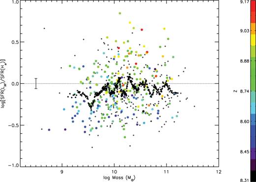
log SFR(Hα)–log SFR(L_IR) versus log Mass. The black dots are the running mean of Δ(SFR) every 20 values of stellar mass, while the colours represent different metallicity values. Also shown at the left hand of the plot is the typical mean error of the running mean.

Open in new tabDownload slide

We should remind that our SFR(Hα) is also affected by errors and systematic uncertainties on its derivation. Brinchmann et al. (2004) (hereafter B04) have shown that, differently from what is assumed in equation (4), the ratio of observed Hα luminosity to SFR, i.e. the efficiency η = L_Hα/SFR, is not constant, but depends on the mass of the galaxy, with higher values for lower mass systems. Therefore, the mass dependence that we observe could be due to the fact that we are overestimating the SFR(Hα) for low-mass systems.

To address this issue, we have re-calculated our SFR(Hα) making use of the B04 recipes. In this work, the authors derive different η values for different mass ranges. Even using mass-dependent efficiencies, the disagreement between the two SFR indicators at lower masses is still present, while the slope of the SFR(L_IR)–SFR(Hα) relation remains consistent with the one-to-one relation (m = 0.95 ± 0.03). As a further improvement, in B04 the authors also derive a mass-dependent extinction value for the Hα emission line. We have also calculated the SFR values using both the mass-dependent efficiency and the mass-dependent extinction from B04 (instead of using the extinction values derived from equation (2)). When including the extinction values derived from B04, the disagreement at lower masses is slightly reduced, but now the values of the SFR(L_IR) are significantly higher than the SFR(Hα) at higher masses. Moreover, the slope of the SFR(L_IR)–SFR(Hα) relation derived using the B04 extinction values is significantly larger than 1 (m = 1.26 ± 0.05). This is mainly due to the fact that the B04 extinction values at high L_IR are lower than the extinction values that we derive from equation (2).

6.3 Metallicity

A physical parameter related to the mass is the metallicity. Metallicity and mass are correlated by the well-known mass–metallicity relation (Tremonti et al. 2004), with more massive galaxies being more metal-rich, at least up to M ∼ 10M_⊙. Above this mass, metallicity still increases with mass, but the slope of the relation is significantly flatter than at lower masses. Therefore, the difference between SFR(Hα) and SFR(L_IR) could also be due to the different metal content of the galaxies. To test this effect we have made use of the COSMOS metallicity catalogue by Nair et al. (in preparation), using the Denicoló, Terlevich & Terlevich (2002) method to estimate metallicity from [N II] and Hα emission lines. In Fig. 8 we have plotted our sources with different colours for different metallicity values (black crosses represent galaxies for which the metallicity measurement is not reliable, 48 per cent of the sample). It can be seen that the lower values of the SFR(L_IR) at low masses is mainly driven by a small number of very metal poor galaxies, while most of the most metal rich galaxies lie above the zero-point.

To better appreciate the dependence of the two SFR indicators from metallicity, in Fig. 9 we show the ratio between the two SFR indicators versus the metallicity. The red dots are the running mean of Δ(SFR) = log SFR(L_IR)−log SFR(Hα) every 20 values of Z. Also shown in the left hand of the plot is the typical mean error of the running mean (σ_{rm, Z} = 0.07). It can be observed that for metal-poor galaxies the SFR(L_IR) values are lower than the SFR(Hα), while for metal-rich galaxies the SFR(L_IR) values are larger. The average difference between the two SFR indicators varies by ∼0.6 dex when moving from the metal-poor to the metal-rich galaxies, meaning that the metallicity has a very important effect when deriving the SFR. This is consistent with the fact that more metal-rich galaxies usually have higher dust to gas ratios (Baugh et al. 2005; Schurer et al. 2009), meaning that more metal-rich galaxies are more efficient in absorbing and re-emitting the light emitted by young stars at IR wavelengths (at least until the optical depth in the UV goes over τ > 1). Therefore, for the same SFR values, a metal-rich galaxy emits more in the IR; thus the SFR derived from the L_IR is overestimated with respect to the SFR from the Hα luminosity. We remind that the K98 relation is calibrated for solar metallicity and note that for that value [12+log(O/H) = 8.69; Asplund et al. 2009] the agreement between the two SFR indicators is very good.

Figure 9.

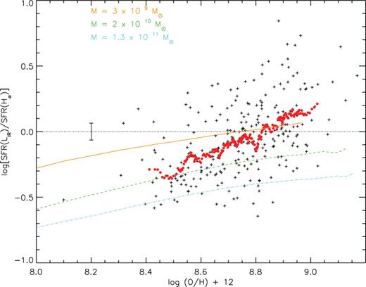
Log SFR(L_IR)–log (Hα) versus metallicity. Red dots are the running mean of Δ(SFR) every 20 values of Z. The coloured lines represent the result for the chemo-spectrophotometric model for three spiral galaxies of different masses (see Section 6.4).

Open in new tabDownload slide

It could be argued that the observed trend with metallicity could be also affected by using the linear relation between log L_IR and E(B − V) for all the galaxies. For metal-poor galaxies, the dust extinction correction that we apply could be larger than the actual one; thus the SFR(Hα) that we derive would be biased high, leading to the low values of the ratio between the two SFR indicators at low metallicities. However, even when using the B04 recipes to derive the SFR, which include both a mass-dependent efficiency and a mass-dependent dust extinction, the ratio between the two SFR estimates was still very different for metal-poor and metal-rich galaxies. We eliminated the scatter due to the metallicity dependence on the SFR comparison, finding a reduction of the dispersion of 14 per cent (from σ = 0.28 to σ = 0.24). We conclude that metallicity is a key parameter when deriving the SFR and suggest that the K98 relation cannot be applied blindly when considering very metal poor/rich galaxies.

6.4 Comparison with a model for dust evolution in spiral galaxies

A suite of chemical evolution models for spiral galaxies able to reproduce the observed evolution of the mass–metallicity relation has been presented in Calura et al. (2009). In that work, three spiral models, representing galaxies of different masses, have been designed in order to reproduce a few basic scaling relations of disc galaxies across a stellar mass range spanning from 10⁹ M_⊙ to 10¹¹ M_⊙. In such models, it was assumed that the baryonic mass of any spiral galaxy is dominated by a thin disc of stars and gas in analogy with the Milky Way (MW). The disc is approximated by several independent rings, 2 kpc wide, without exchange of matter between them. The time-scale for disc formation is assumed to increase with the galactocentric distance, according to the ‘inside-out’ scenario (Matteucci & Francois 1989). The models for spiral discs include dust production, mostly from core-collapse supernovae and intermediate-mass stars, restoring significant amounts of dust grains during the AGB phase, as well as dust destruction in supernova shocks and dust accretion. The prescriptions for dust production are the same as in Calura, Pipino & Matteucci (2008), where a chemical evolution model for dust was presented, able to account for the observed dust budget in the MW disc, in local ellipticals and in dwarf galaxies. In a subsequent work, Schurer et al. (2009) combined the predicted dust masses and the star formation history of the MW galaxy with a spectrophotometric evolution code that includes dust reprocessing (Graphite and Silicate; GRASIL).

The relation between log [SFR(L_IR)/SFR(Hα)] and metallicity observed in spiral galaxies is compared with the results from chemo-spectrophotometric models of three spiral galaxies of different masses in Fig. 9. In the model, the SFR(L_IR) quantity is calculated according to equation (4), where the total IR luminosity L_IR of the spiral galaxy has been calculated by integrating the SED in the range 8–1000 μm. In Fig. 9, the metallicity [expressed as log (O/H) +12] is a direct output of the chemical evolution models of Calura et al. (2009). Here, the quantity SFR(Hα) is the intrinsic SFR ψ, calculated by means of the Schmidt–Kennicutt law

5

where σ is the gas density per unit surface and k ∼ 1.5. In agreement with what is observed in real galaxies, in the three models the ratio log [SFR(L_IR)/SFR(Hα)] grows with metallicity. This is due to the fact that, as galaxies evolve, their interstellar metallicity rises and their SFR decreases, accompanied by a milder decrease in the FIR luminosity. In the model, the smaller decrease of the FIR luminosity with respect to the SFR reflects the fact that the FIR luminosity is only to a first-order approximation proportional to the SFR; in fact, significant contributors to dust production and heating are also intermediate-mass stars, whose total mass within a galaxy reflects the integrated star formation history. Our models predict a larger log [SFR(L_IR)/SFR(Hα)] value at a fixed metallicity for lower mass galaxies. It is also worth noting that the observed increase of the log [SFR(L_IR)/SFR(Hα)]–metallicity relation is stronger than the model results, with a substantial number of the observed systems presenting log [SFR(L_IR)/SFR(Hα)] > 0.1, not reproduced by our models. The majority of these systems have metallicities 12 + log (O/H) > 8.5, but do not present particularly high SFR or stellar mass values. There are two possible reasons for this discrepancy between the model results and the observed galaxies.

One possibility is that the star formation history of the three spiral models does not represent the true star formation history of the observed galaxies; a significant number of real galaxies may have more complicated star formation histories, for instance characterized by episodic starbursts, as opposed to our models, characterized by smooth star formation histories. Another possibility is that, for these relatively high metallicity systems, the corrected SFR(Hα) values may represent lower limits to the intrinsic SFR values. It could be that, the larger the metallicity and the dust content of the galaxy, the more likely are the star-forming regions to become thick to Hα radiation. One consequence may be that particularly optically thick regions may be missed, and that the total SFR rate determined from Hα emission may be underestimated. At present, it is very difficult to assess which one of the two possibilities may be the main cause of our discrepancy. A useful test in this regard would imply the use of spectrophotometric models including the effects of dust extinction on nebular emission lines (e.g. Panuzzo et al. 2003). The combined use of such models with chemical evolution models including dust evolution will be an interesting subject for future work and will likely shed more light on the main subject of this paper.

6.5 SSFR

The SSFR is a very interesting parameter as it does not only account for the number of stars being formed, but also takes into account the efficiency of a galaxy of a given mass to form stars with respect to its total mass content. It gives information about the star formation activity of a galaxy, allowing us to divide them into star-forming, active or intermediate galaxies. It is reasonable to consider that galaxies with different star formation modes may show different luminosity–SFR relations. In Fig. 10 we show a similar plot to Fig. 8 where now the considered parameter is the SSFR and the colours represent different ages of the galaxies derived by means of the SED fitting (calculated when deriving the galaxy stellar masses as explained in Section 3.2). Also shown is the typical mean error of the running mean (σ_{rm, SSFR} = 0.06). The SFR value that we use in this plot is the mean value of SFR(Hα) and SFR(L_IR). This value has been chosen to avoid a systematic trend with one of the two SFR indicators, which are present in the y-axis. As expected, all of our galaxies have high values of SSFR and would be classified as star-forming galaxies following different criteria recently found in the literature (see e.g. Pozzetti et al. 2010; Domínguez Sánchez et al. 2011).

Figure 10.

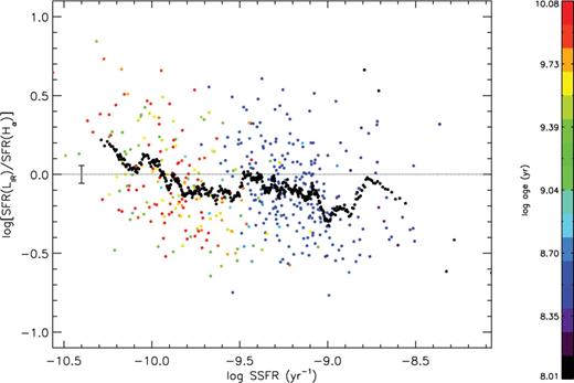
Log SFR(L_IR)–log SFR(Hα) versus SSFR. Colours represent the galaxy stellar ages as derived from the SED fitting. The black dots are the running mean of Δ(SFR) every 20 values of SSFR and the error bar at the left hand of the plot is the typical mean error of the running mean.

Open in new tabDownload slide

We observe values of the SFR(L_IR) larger than the SFR(Hα) by ∼0.2 dex for galaxies with small values of SSFR (<10.0 [yr⁻¹]). A possible explanation for these higher values of SFR(L_IR) at low SSFRs is the fact that the old stellar population may significantly contribute to the L_IR of a galaxy as already mentioned by K98 (see also a recent work by da Cunha et al. 2011). For the galaxies with low SSFR, the heating by stars older than 10⁷ years in the diffuse inter stellar medium can be comparable to the dust luminosity from the absorption of light from young stars; thus the value of the SFR(L_IR) is overestimated as it includes emission from the old stellar population and not only from the recently formed stars. In fact, as it can be seen in Fig. 10, the oldest galaxies (redder colours) populate the low SSFR region of the plot, while the galaxies with the youngest stellar populations (bluer colours) have always larger SSFR inferred values. Another possible explanation for the observed trend between the two SFR indicators with SSFR could be due to spikes in recent SFR. A galaxy undergoing a current burst (high SSFR) will have a high Hα flux compared with its L_IR and the log [SFR(L_IR)/SFR(Hα)] will take negative values, with the opposite trend happening for low SSFRs. Again, this trend is not reduced when using B04 recipes to estimate the SFR(Hα). Finally, we would like to remark that the results from Figs 9 and 10 are in agreement with the fundamental metallicity relation observed by Mannucci et al. (2010), where the authors find that a decrease in metallicity also correlates with an increase in SSFR. The SFR(L_IR) seems to be higher, on average, than the SFR(Hα) both for galaxies with high metallicity and for galaxies low SSFR values.

We conclude that caution must be taken when deriving the SFR from the L_IR for galaxies with low values of SSFR, as the emission from the older stellar population may overestimate the derived SFR. The opposite effect may happen for galaxies with recent star formation bursts, i.e. high SSFR values.

6.6 Morphological type

Another important property that could affect the SFR indicators is the morphological type, as different morphologies are associated with different star formation histories and geometries and therefore different SEDs and IR emission. To assess the effect of morphology on the SFR derivation we have made use of the morphological catalogue by Nair et al. (in preparation), who, following a similar scheme as in Nair & Abraham (2010), visually classified the galaxies belonging to the COSMOS field, dividing them into different types (Ell, S0, Sa-Sd, Irr). In Fig. 11 we show the usual log SFR(L_IR) versus log SFR(Hα) plot dividing our sample into different morphological types.

Figure 11.

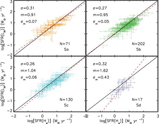
Log SFR(L_IR) versus log SFR(Hα) for sources classified as Sa, Sb, Sc or Sd/Irr. Red dashed and continuous lines are the best fit to our data and the one-to-one relation, respectively. Also shown are the derived values for the slope (m) and its error (σ_m), as well as the scatter of the relation (σ) and the number of sources for each morphological type.

Open in new tabDownload slide

The two SFR indicators are in very good agreement with each other for the three spiral sub-samples. For each of them the SFR(L_IR)–SFR(Hα) relation is consistent, in both normalization and slope, with the one-to-one relation. For the Sd, irregular sample (Sd/Irr), the formal best-fitting slope becomes much steeper (m = 1.62 ± 0.43), but is still consistent with 1 at the 1.5σ level, because of the reduced statistics of this sub-sample (we have only 17 sources classified as Sd or irregular galaxies.). The dependence of the SFR indicators with morphology has also been studied by Kewley et al. (2002), finding that the ratio between SFR(L_IR) and SFR(Hα) is almost the same for early (S0-Sab) and late (Sb-Irr) type galaxies. If real, one possible explanation for the discrepancy for the Irr/Sd galaxies is their complex morphology. Irregular galaxies are clumpier and less homogeneous than earlier spiral galaxies, thus making it more difficult and uncertain to measure the total Hα flux of the galaxy due to aperture corrections. We have also investigated the possible effect of metallicity in the Sd/Irr sample, as irregular local galaxies are found to be metal poor (Tolstoy, Hill & Tosi 2009). However, we did not see a different metallicity distribution for the Irr/Sd sample than for the whole sample of galaxies. Despite the fact that the number of Sd/Irr objects is quite small, we observe a slight trend of a steepening of the slope of the SFR(L_IR)–SFR(Hα) relation when moving from early to late spiral galaxies. For example, if we analyse together Sa and Sb galaxies we obtain a slope of m = 0.93 ± 0.04, i.e. almost a 3σ difference with respect to the slope for the Sc sample. This difference may be indicative of a weak dependence of the SFR indicators with morphology. However, a more significant statistical sample would be necessary to assess if the observed steepening of the slope with morphological type is a real effect or if it is just due to the few sources considered for each morphological type, especially for the Sd/Irr sample.

7 Summary and Conclusions

In this paper we have empirically tested the relation between the SFR derived from the L_IR and the SFR derived from the Hα emission line. We have studied a sample of 474 galaxies at z = 0.06–0.46 with both Hα and IR detection from 20k zCOSMOS and PEP Herschel at 100 and 160 μm. The L_IR has been derived by integrating from eight to 1000 μm the best-fitting SED to our IR data from IRAC, Spitzer and Herschel. We have derived our SFR from the Hα extinction corrected emission line. We have constructed six average spectra with different average L_IR values and we have found a very clear trend between E(B − V) and log L_IR. This allows us to estimate E(B − V) values for each galaxy (see equation (2)) even if the quality of the spectra does not allow us to accurately measure the Hβ emission line for each galaxy. Our main conclusions are as follows.

• (i)

  We have compared the SFR(L_IR) and SFR(Hα) finding an excellent agreement between the two SFR estimates for the bulk of the studied galaxies, with the slope of the SFR(L_IR)–SFR(Hα) relation m = 1.01 ± 0.03 and the normalization constant of a = −0.08 ± 0.03. This means that the simple recipes used to convert luminosity into SFR by simply scaling relations are consistent with each other. The agreement between the two SFR estimates also implies that the assumptions, for example on star formation histories, that were made to derive the SFR recipes (equations 1 and 4) should not be very different from the properties of the studied sample. The comparison of the SFR indicators at low redshift is crucial to test the validity of the SFR estimates which are often used in high-redshift studies. The main result that we obtain is that both methods are in very good agreement for the low-redshift sample, allowing us to extend their validity at higher redshifts. This allows us to derive the SFR of distant galaxies when only the L_IR or the Hα information are available, with the assurance that we are not introducing important systematic effects.

• (ii)

  There seems to be no dependence of the SFR indicators with redshift, at least up to z ∼ 0.46, which is the limit of our sample.

• (iii)

  The stellar mass seems to have a small influence on the SFR(L_IR)–SFR(Hα) relation in the sense that for low-mass galaxies the SFR(L_IR) values are lower than the SFR(Hα). However, the observed dependence of the SFR indicators with the stellar mass seems to be mainly driven by metallicity.

• (iv)

  The metallicity, in fact, seems to be the parameter that most influences the SFR comparison, with average values of log [SFR(L_IR)/SFR(Hα)] which differ by ∼0.6 dex from metal-poor to metal-rich galaxies. This is due to the higher efficiency in absorbing and re-emitting the light from young stars in the IR for more metal-rich galaxies. The dispersion of the SFR(L_IR)–SFR(Hα) relation is reduced by 14 per cent when taking into account the scatter due to the metallicity. We stress that caution must be taken when deriving SFR for very metal poor/rich galaxies.

• (v)

  We show how the behaviour of the observed SFR(L_IR)/SFR(Hα)–metallicity relation finds a natural explanation within the frame of a complete theoretical model for dust evolution in spiral galaxies.

• (vi)

  The SFR(L_IR) values are larger than the SFR(Hα) for galaxies with low SSFR values (log SSFR < 10 [yr⁻¹]) probably due to the non-negligible contribution to the IR emission from the old stellar population. Stars older than 10⁷ years may significantly contribute to the L_IR in systems with little star formation activity. The difference between the two estimates could also be affected by the effect of short and intense bursts of star formation, i.e. galaxies with high SSFR values.

• (vii)

  When separately studying the SFR indicators as a function of morphological types, we find that they are in excellent agreement with each other for the three spiral sub-samples. For each of them the SFR(L_IR)–SFR(Hα) relation is consistent, in both normalization and slope, with the one-to-one relation. For the Sd, irregular sample (Sd/Irr), the formal best-fitting slope becomes much steeper (m = 1.62 ± 0.43), but is still consistent with 1 at the 1.5σ level, because of the reduced statistics of this sub-sample.

Acknowledgments

This work was supported by an international grant from Instituto de Astrofísica de Canarias (IAC) with funding from the Research Structure Departments of Instituto Nazionale di Astrofisica (INAF). PACS has been developed by a consortium of institutes led by MPE(Germany) and including UVIE (Austria), KU Leuven, CSL, IMEC (Belgium), CEA, LAM (France), MPIA (Germany), INAF-IFSI/OAA/OAP/OAT, LENS, SISSA (Italy), IAC (Spain). This development has been supported by the funding agencies BMVIT (Austria), ESA-PRODEX (Belgium), CEA/CNES (France), DLR (Germany), ASI/INAF (Italy) and CICYT/MCYT (Spain). We thank the COSMOS/zCOSMOS teams for making the data available for the community and the anonymous referee for a constructive report.

References

PEP images and catalogues will be released at http://www.mpe.mpg.de/ir/Research/PEP/public_data_releases.php (see also Lutz et al. 2011)