


ABSTRACT
The background noise between 1 and 1.8 μm in ground-based instruments is dominated by atmospheric emission from hydroxyl molecules. We have built and commissioned a new instrument, the Gemini Near-infrared OH Suppression Integral Field Unit (IFU) System (GNOSIS), which suppresses 103 OH doublets between 1.47 and 1.7 μm by a factor of ≈1000 with a resolving power of ≈10 000. We present the first results from the commissioning of GNOSIS using the IRIS2 spectrograph at the Anglo-Australian Telescope. We present measurements of sensitivity, background and throughput. The combined throughput of the GNOSIS fore-optics, grating unit and relay optics is ≈36 per cent, but this could be improved to ≈46 per cent with a more optimal design. We measure strong suppression of the OH lines, confirming that OH suppression with fibre Bragg gratings will be a powerful technology for low-resolution spectroscopy. The integrated OH suppressed background between 1.5 and 1.7 μm is reduced by a factor of 9 compared to a control spectrum using the same system without suppression. The potential of low-resolution OH-suppressed spectroscopy is illustrated with example observations of Seyfert galaxies and a low-mass star.
The GNOSIS background is dominated by detector dark current below 1.67 μm and by thermal emission above 1.67 μm. After subtracting these, we detect an unidentified residual interline component of ≈860 ± 210 photons s−1 m−2 arcsec−2 μm−1, comparable to previous measurements. This component is equally bright in the suppressed and control spectra. We have investigated the possible source of the interline component, but were unable to discriminate between a possible instrumental artefact and intrinsic atmospheric emission. Resolving the source of this emission is crucial for the design of fully optimized OH suppression spectrographs. The next-generation OH suppression spectrograph will be focused on resolving the source of the interline component, taking advantage of better optimization for a fibre Bragg grating feed incorporating refinements of design based on our findings from GNOSIS. We quantify the necessary improvements for an optimal OH suppressing fibre spectrograph design.
1 Introduction
Observations at near-infrared (NIR) wavelengths are severely hindered by the night-sky background. The night-sky surface brightness is ≈14.9 AB mag arcsec−2 in the H band, compared to ≈21.1 AB mag arcsec−2 in the V band. This results in high Poisson noise in any observation. Compounded with this, the night-sky brightness varies by factors of ≈10 per cent on the time-scale of minutes (Ramsay, Mountain & Geballe ; Frey et al. ), with a further gradual dimming of about a factor of 2 throughout the night (Shimazaki & Laird ). This temporal variability results in a high systematic noise when performing sky subtraction, which is not trivial to remove (e.g. Davies ; Sharp & Parkinson ).
In the J and H bands, the dominant sources of background are the Meinel bands of emission lines resulting from the rotational and vibrational de-excitation of OH molecules (Meinel ; Dufay ). We have reviewed the NIR background, and in particular the characteristics of the OH emission line spectrum in an earlier paper (Ellis & Bland-Hawthorn ). We note that although they are very bright, the OH lines are intrinsically narrow (full width at half-maximum, FWHM ≈ 3 × 10⁻⁷ μm), and between the OH lines the night-sky background should be very faint, possibly as low as ≈100 photons s−1 m−2 arcsec−2 μm−1 if the background is dominated by zodiacal scattered light, and is likely to be at least as faint as ≈600 photons s−1 m−2 arcsec−2 μm−1 as shown by R = 17 000 spectroscopic observations made by Maihara et al. (). Thus, if the OH lines can be efficiently filtered from the night-sky spectrum, whilst maintaining good throughput between the lines, it should be possible to achieve a dark background in the NIR, allowing much deeper observations than possible hitherto.
This paper presents the first results from an instrument designed to achieve exactly this efficient filtering of the OH skylines. The filtering is achieved using fibre Bragg gratings (FBGs). FBGs were originally developed for use in telecommunications and required significant modification to be used for OH suppression (see Bland-Hawthorn et al. for a comprehensive treatment on the physics of OH suppression with FBGs). First, it was necessary to significantly increase the number of notches in each grating (typically only one notch is used in devices used in telecommunications) and the wavelength range of the devices which were available at the time, a breakthrough which was enabled with the design of aperiodic FBGs (Bland-Hawthorn, Englund & Edvell ). Secondly, it was required to develop a multimode (MMF) to single-mode fibre (SMF) converter (Leon-Saval et al. ; Noordegraaf et al. ), since at the plate scale of typical telescopes the narrow core of an SMF has too small a field of view to collect an adequate amount of light from the seeing disc. Subsequent refinement (Bland-Hawthorn, Buryak & Kolossovski ; Bland-Hawthorn et al. ) has resulted in the latest FBGs being able to suppress 103 notches over a wavelength range of 230 nm, which is achieved using two devices in series.
Ellis & Bland-Hawthorn () presented the potential benefit for the astronomy of OH suppression with FBGs and described the expected performance. They pointed out that a key benefit of OH suppression with FBGs compared to other previously suggested methods of OH suppression (e.g. high-dispersion masking; Maihara & Iwamuro ) is that the OH light is removed before it enters the spectrograph and in a manner dependent only on wavelength. Hence, the interline continuum is not contaminated with scattered OH light within the spectrograph which can otherwise dominate other sources of the interline continuum. The testing of this prediction was a central goal of GNOSIS commissioning.
The first on-sky tests of OH suppression with FBGs were performed at the Anglo-Australian Telescope (AAT) in 2008 December. This experiment consisted of two MMFs pointed directly at the sky through a hole in the AAT dome wall. Both fibres fed a 1 × 7 photonic lantern (see Section ), one of which had FBGs inserted and the other did not, to serve as a control. The results of these tests are described in Bland-Hawthorn et al. (, ) and demonstrated the clean suppression of the OH lines. However, since each fibre accepted light from an ≈12° patch of sky, these tests could not perform observations of individual sources, nor could they measure the interline continuum since every observation included light from many stars and other sources.
We have designed, built and commissioned the first instrument to use FBGs for OH suppression. GNOSIS is an OH suppression unit designed to feed the IRIS2 infrared imaging spectrograph at the AAT (Tinney et al. ). The name is an acronym for Gemini Near-infrared OH Suppression IFU System, revealing the intention to install a similar system on the GNIRS spectrograph at Gemini North (Elias et al. ,,) at a future date. A summary of description of the instrument is given in Section . In this paper, we concentrate on the performance and results of the OH suppression. We describe the observations in Section , and we present the results in Section giving details of throughput, sensitivity and background. The NIR background will be examined in detail in a future paper (Trinh et al., in preparation), examining the various components of the background and their dependence on moonlight, ecliptic latitude, air mass, Galactic latitude, etc.; a brief description of the main components will be given here. In Section , we present observations of two Seyfert galaxies and an L/T dwarf illustrative of OH suppression. In Section , we discuss our results in the context of the benefit of OH suppression to NIR spectroscopy and in the context of lessons for future OH-suppressed instruments.
2 GNOSIS
The optical light path for GNOSIS is illustrated in Fig. 0001. A seven-element lenslet array accepts light from the f/8 Cassegrain focus and feeds this to seven 50 μm core fibres. The individual lenslets subtend a width (from face to face) of 0.4 arcsec on the sky. Each of the 50 μm core fibres is capable of carrying ≈79 modes, but light is injected at less than the full numerical aperture of the fibres (i.e. a slower beam) such that only ≈19 modes are carried. These fibres are spliced into a photonic lantern (Leon-Saval et al. ; Noordegraaf et al. ), which converts an MMF into a parallel array of SMFs via a fibre taper, and in the case of GNOSIS, into 19 SMFs since there are 19 modes per fibre. These SMFs are each spliced into two FBGs in series which suppress the 206 brightest OH lines (i.e. 103 closely spaced Λ doublets) between 1.47 and 1.7 μm. These FBGs are then spliced into a reverse photonic lantern converting each of the 7 × 19 SMFs back into seven MMFs. These are connected to a 12 m fibre run which leads to IRIS2, located on the dome floor beneath the telescope. The ends of the fibres form a pseudo-slit, the output of which is re-imaged via two lenses into IRIS2. A custom slit mask within IRIS2 blocks extraneous light. IRIS2 has a Rockwell Hawaii-1 detector with 1024 × 1024 pixels, a dark current of 0.015 e− s−1 and an effective read noise of ≈8 e− when using an up-the-ramp non-destructive read-out mode. The point spread function (PSF) of GNOSIS with IRIS2 was measured to be 2.0 pixel FWHM, which gives a spectral resolving power of λ/Δλ ≈ 2350. The mean dispersion was measured to be ≈3.5 Å pixel−1. A full description of the instrument may be found in a forthcoming paper (Trinh et al., in preparation).

A schematic diagram of the components of the GNOSIS instrument, as described in Section 2.
The properties of the GNOSIS system are given in Table 0001. These include properties of GNOSIS per se and also those properties of IRIS2 on which GNOSIS observations depend. The observed wavelength range is defined by the spectrograph and the blocking filter, and is larger than the OH-suppressed range which is that of the FBGs.

Properties of the GNOSIS system
3 OBSERVATIONS
GNOSIS was commissioned on five separate observing runs in March, May, July, September and November of 2011. In this paper, we present only observations from the September and November commissioning runs, which incorporate the improvements made to the instrument in the previous commissioning runs. The observations presented are listed in Table 0002. We present four different experiments: (i) measurement of the instrument throughput from standard star observations, (ii) measurement of the night-sky background, (iii) measurement of the instrument sensitivity by observations of a low surface brightness galaxy and (iv) observations of Seyfert galaxies illustrating the benefits of OH suppression.
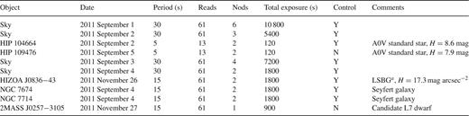
GNOSIS observations
All observations were made using an up-the-ramp read mode to minimize the effect of detector read noise; we have recorded the period and number of reads in Table 0002; the final exposure time for an individual frame is (reads − 1) × period. All observations of objects included an equal amount of time spent on the sky and followed an object–sky–sky–object pattern. We denote the total number of object frames as ‘Nods’ in Table 0002. For observations on September 1–4, we disconnected an MMF from the grating unit to provide a control fibre with no OH suppression, as indicated in the ‘Control’ column of Table 0002.
3.1 Data reduction
We reduced the data using a bespoke code written as a mathematica notebook, except for the first step of collapsing the data cubes (see Section ), which was performed using a C program. Since the night-sky background is considerably reduced using OH suppression, the issue of correctly accounting for the effects of detector noise becomes very important, and we have paid careful attention to this in our data reduction. Our procedure was as follows.
3.1.1. Collapsing the data cubes
For each frame, the detector was used in a multiple-read mode (MRM) using an up-the-ramp sampling, with intervals of either 5, 15 or 30 s and either 13 or 61 reads (see Table 0002). This means that the detector is reset, and then read non-destructively at a fixed time interval for a specified number of times. This enables non-linearity in the detector response to be removed. Upon investigation we found significant non-linearity in the first few reads. For dark frames with the blank filters in, if one always observes in MRM, then the first read after reset is higher than the second read, and thereafter the counts are linear until about 20 000 ADU (see Fig. 0002a). If the MRM exposure follows a double read mode (DRM) observation (i.e. only two reads immediately prior to and after the exposure), then the first approximately five reads show a decline in the bias levels (see Fig. 0002b). This effect has been seen by one of us (AJH) in other Hawaii-1 PACE detectors. The largest observed drop in bias levels in the first few reads is ≈15 ADU, which is insignificant under typical non-OH-suppressed observations since the brightness of the night sky swamps such small variations. Thus, for normal NIR observations a linear least-squares fit to the reads suffices to recover the incident count rate. However, in the case of OH-suppressed observations, this is no longer so, since the incident count rate can be very low for pixels between the OH lines. Therefore, we have simply dropped the first five reads from our data cubes before performing a linear least-squares fit to the remaining data. The slope of this fit is then multiplied by the original number of reads minus 1 to recover the true incident count rate.
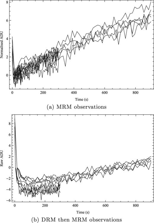
The dark current in raw ADU for the IRIS2 detector. The data have been normalized to zero for the second read. The top plot shows data if the detector is always read in the MRM mode. The bottom plot shows data if the MRM frame is preceded by a DRM frame.
3.1.2. Detector linearity
The detector non-linearity due to the filling of the pixel wells is mitigated by keeping the counts per pixel below 20 000 ADU. Thus, in collapsing the data cubes as described above, we use a linear least-squares fit. Thereafter, we correct for any non-linearity following the procedure given on the IRIS2 web pages (http://www.aao.gov.au/AAO/iris2/iris2_linearity.html).
3.1.3. Background subtraction
The GNOSIS background consists of dark current, instrument thermal background, telescope thermal background and the night-sky background (including OH emission, thermal emission, zodiacal scattered light, moonlight, etc.). For our object observations, we nod the telescope between the object and the sky, and thus all the background can be subtracted simultaneously using the sky observations. Pairs of observations are first subtracted, and then averaged using the median if there are more than two.
For our sky observations, this is not possible. In this case, we subtract the dark current and the thermal background separately. The dark current is subtracted using the median of several dark frames of the same read mode and exposure time as the observations.
We have measured the thermal component from ‘cold frame’ observations. A cold frame is an observation for which the GNOSIS fore-optics were removed from the Cassegrain focus and pointed directly into a dewar filled with liquid nitrogen. Thus, the cold frame contains the GNOSIS fore-optics and IRIS2 thermal backgrounds and the detector dark current alone. The telescope thermal background should be much lower than the instrument background since the emissivity from the mirror should be less than 3 per cent, and the emissivity from the Cassegrain hole is from a much smaller solid angle.
The average cold frames are shown in Fig. 0003. The counts have been calibrated to reproduce a T = 282 K, 100 per cent emissivity blackbody, i.e. the expected emission from the slit block, etc. at the output end of GNOSIS. This calibration provides an independent check on the efficiency of IRIS2 as discussed in Section .

The smoothed GNOSIS thermal background (continuous line) normalized to a T = 282K blackbody, i.e. the ambient dome temperature at the time of observation (dashed line).
Obtaining cold frames is a significant overhead on observing time since the fore-optics must be removed, and then refitted and re-aligned during the night when the optics are at the same temperature as for the sky frames. Thus, in practice we fit a blackbody spectrum to our observations by choosing regions of the continuum between the OH lines with λ > 1.7 μm. The best-fitting model is subtracted from observations. We note that thermal emission is only approximately blackbody (see Fig. 0003). However, a more general function may inadvertently fit and subtract intrinsic features of the sky emission. Since we do not know the exact function of the thermal emission, we revert to an approximate but physically motivated blackbody fit. An example of blackbody fit is shown in Fig. 0004. This is actually done after the residual background correction step detailed in Section .

An example fit (thick, black line) to the GNOSIS thermal background which is assumed to be given by the points located between the OH lines in the night-sky spectrum (thin line).
3.1.4. Spectral extraction
Spectroscopic observations of the illuminated dome flat-field screen were taken to provide a trace of the spectra across the detector. The centre of each of the seven spectra is calculated at each spectral pixel. This is done by fitting the sum of seven Gaussians to the pixel counts in the spatial direction at each spectral pixel. The Gaussians for each fibre are assumed to have identical σ and to be equally spaced. The fit yields the centre of each Gaussian, and this is stored in a look-up table, along with the σ of the Gaussian fit. The separation between the spectra is 11 pixels, which is ≈5.5 times the FWHM of the PSF, and therefore cross-talk between the spectra is negligible.
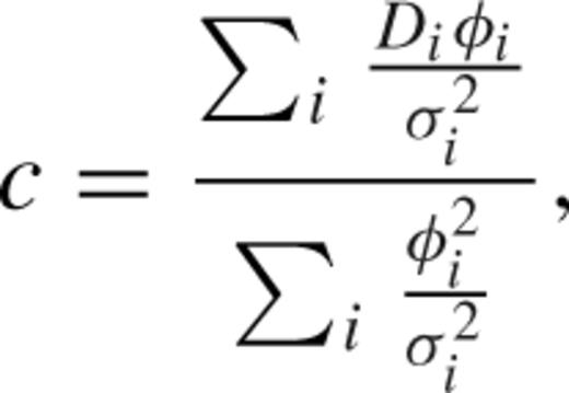
 the pitch between spectra, Di is the count at each pixel,
  is the variance on the count and ϕi is the value of the normalized Gaussian profile at that pixel. This method minimizes the contribution due to noise in the extraction.
3.1.5. Fibre to fibre variations
We next correct for variations in the throughput between fibres. The fibre-to-fibre variation is measured from dispersed images of the illuminated dome flat-field screen which are extracted in the same manner as the object spectra. The normalized fibre-to-fibre variation is the ratio of the total flux in each spectrum to the average of the total flux of all seven spectra. The extracted spectra are divided by the normalized variation.
3.1.6. Spectral combination
The seven extracted spectra are combined by taking the sum of each spectral pixel. If a control fibre was used, this is excluded from the combination. This step neglects to take into account differences in the wavelength solution of each spectrum, which are less than 1.5 pixels over most of the detectors. We have checked that not correcting for these differences does not introduce spurious signals by repeating the reduction of the sky spectrum for a single fibre only. We find that the single extracted spectrum is consistent with the summed spectrum.
3.1.7. Wavelength calibration
The wavelength calibration is achieved using Xe arc lamp spectra. These spectra are extracted and combined as described above. The Xe lines are automatically detected, and a cubic polynomial is fitted to give the wavelength as a function of the spectral pixel number. This solution is then applied to the object spectra. The wavelength calibration is accurate to ≈2 Å and is limited by the slight shift in the dispersion solution for each spectrum.
3.1.8. Residual background subtraction
Hawaii-1 detectors are known to suffer from significant interquadrant cross-talk (Tinney, Burgasser & Kirkpatrick ); if a bright object appears at pixel {x, y}, then there will also be a faint glow at pixel {x, mod(y + 512, 1024)} (where mod is the modulo operation) and along the entire row x. The cross-talk between quadrants does not affect GNOSIS observations, since all seven spectra are located on the lower two quadrants, but the cross-talk along rows does.
The cross-talk along a row can be measured in the region of the spectrum at λ < 1.45 μm, since this region ought to be completely dark due to the spectroscopic blocking filter. This measurement may also include other residual background from systematic errors in the previous subtraction due to changing background levels. We measure the mean count rate at λ < 1.45 μm and subtract it from the spectrum.
3.1.9. Instrument response and telluric correction
The efficiency of the GNOSIS system, including the atmosphere, the telescope and IRIS2, is measured from observations of A0V stars. These observations are reduced as described in the previous steps. We then take a model spectrum of Vega (Castelli & Kurucz ) and divide the observations by this to give a relative throughput of the system as a function of wavelength, including telluric features. Note that this will also include the averaged pixel-to-pixel variation in our extracted spectra, and hence will include the detector flat-field response. The relative throughput is normalized between 1.5 and 1.69 μm to give the instrument response function. The object spectra are then divided by the instrument response function.
3.1.10. Flux calibration
The observations of the telluric standard stars described in the previous step can also be used to estimate the flux calibration. Since the magnitude of the A0V stars is already known, we can scale the model Vega spectrum to the appropriate brightness before dividing the observed spectrum to yield a flux-calibrated correction. This step is not very accurate since scaling the Vega spectrum relies on knowing the aperture losses of the IFU at the time of observation, which in turn depends upon the seeing and acquisition, which are not readily measurable. The flux calibration is discussed further in Section .
Due to the difficulty of measuring the seeing and the centring of our objects in the IFU, we have computed the aperture losses for a seven-element hexagonal array, assuming the seeing profile is Gaussian. The results are shown in Fig. 0005 as a function of seeing for several values of misalignment. Assuming that we can accurately align to within one element of the IFU, i.e. the offset is ≤0.2 arcsec and the seeing is 1.2 arcsec (extrapolated from measurements taken with the acquisition camera in the I band during the observations), the typical aperture loss for a point source is ≤0.58.
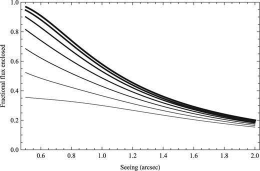
The fractional flux enclosed in the IFU as a function of the seeing. The different curves are for a point source offset from the centre of the IFU by 0, 0.1, 0.2, 0.3, 0.4, 0.5 and 0.6 arcsec going from the thickest to the thinnest lines.
4 RESULTS
We now describe the results of the first three experiments, namely the instrument throughput, the night-sky background and the instrument sensitivity.
4.1 Instrument throughput
4.1.1. Laboratory measurements
The throughput of GNOSIS was measured in the laboratory using a supercontinuum source and an NIR camera (see Trinh et al., in preparation, for details). The total end-to-end throughput of GNOSIS is ≈36 per cent and the throughputs of the individual components are given in Table 0003 with the estimated errors.
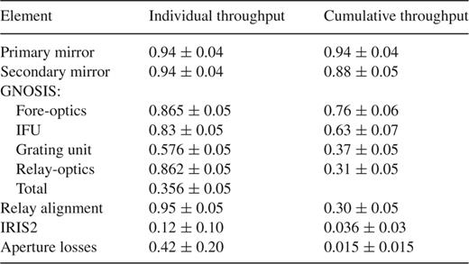
Individual and cumulative throughputs
The throughput of the AAT is approximately 0.942 for the two reflections off the aluminium-coated primary and secondary mirrors, which is estimated from a 0.98 reflectivity of bare Al, combined with an extra 0.96 throughput from the accumulation of dirt on the mirrors. This extra loss is compatible with that measured in the visible on the AAT.
We have estimated the throughput of IRIS2 in two ways. First, we used the IRIS2 imaging exposure calculator to estimate the efficiency of an imaging observation, which for H is ≈29 per cent. Combined with the throughput of the grism (≈40 per cent), this gives a total efficiency of ≈12 per cent. Secondly, we used the observations of the ‘cold frames’ (see Section ) compared to a theoretical blackbody spectrum taking into account the area and solid angle of the IRIS2 slit-mask holes and assuming T = 282 K as recorded and 100 per cent emissivity, since most of the emission will come from the slit block and other mechanical parts surrounding the fibres due to the oversized slit-mask holes. This also yielded an efficiency of 12 per cent.
The end-to-end system throughput is therefore expected to be ≈3.6 or ≈1.5 per cent for a point source including typical aperture losses. We emphasize that this low throughput is not an intrinsic property of OH suppression systems, but is rather a consequence of retrofitting an OH suppression unit to an existing spectrograph, which already has only 12 per cent throughput. The throughput of GNOSIS itself is 36 per cent and is limited mainly by the photonic lanterns. This will be discussed further in Section .
4.1.2. Standard star measurements
We have also measured the end-to-end throughput as a function of wavelength from our observations of A0V stars. Examples are shown in Fig. 0006. The notches in the FBGs are visible as the significant narrow dips in the throughput. Note that in this graph the notches have been convolved with the spectrograph PSF, so they appear shallower than the actual suppression depth. The measurement for HIP 104664 does not include the control fibre. The measured values are very sensitive to seeing and aperture losses as shown in Fig. 0005, but are within the errors of the anticipated throughput estimate in Table 0003. In the case of HIP 109476, the measured throughput would require very low aperture losses due to exceptional seeing, suggesting that some of the values in the table may be pessimistic. However, we assume the conservative values in Table 0003 for the rest of the paper.

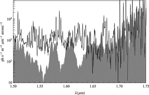
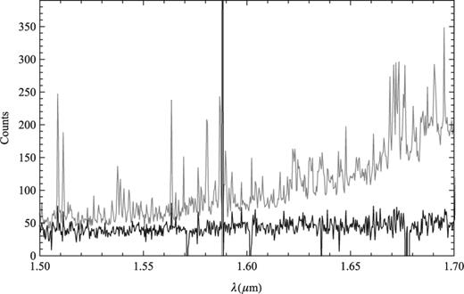
The night-sky spectra for the OH-suppressed observations (red), and the control fibre without OH suppression (blue). The two plots are of the same data; the bottom one has been logged to make the interline regions visible. The pairs of vertical black lines show the OH lines from the Q1(3.5) and Q1(4.5) rotational lines in the 3-1, 4-2 and 5-3 vibrational transitions (from left to right). The green line shows the O2 a-X v=0-1 vibrational line.
4.2 Night sky background
Observations of blank sky were made as targeted observations and as ‘sky frames’ during observations of objects. Fig. 0007 shows the reduced sky spectra for 7.5 h of observations on September 1–4. These data were all >80° from the moon, >50° south of the Galactic plane, >15° off the ecliptic plane and at an air mass <1.5. Therefore, the night-sky spectra should not be significantly contaminated by moonlight, starlight or zodiacal scattered light.

The night-sky spectra for the OH-suppressed observations (red), and the control fibre without OH suppression (blue). The two plots are of the same data; the bottom one has been logged to make the interline regions visible. The pairs of vertical black lines show the OH lines from the Q1(3.5) and Q1(4.5) rotational lines in the 3-1, 4-2 and 5-3 vibrational transitions (from left to right). The green line shows the O2 a-X v=0-1 vibrational line.
4.2.1. OH suppression
The OH lines between 1.5 and 1.7 μm are strongly suppressed. We have measured the suppression factor for 57 doublets; for the remaining 46 doublets, we were unable to obtain a good fit to the unsuppressed line due to either line blending, intrinsic faintness or due to the filter cut-off (at  m). In most cases, the measured strength of the suppressed line is poorly constrained because the flux is so low. Nevertheless, of the 57 doublets, 78 per cent meet or exceed the target specifications.
Some quite bright lines are not suppressed by the FBGs. These are marked with black and green vertical lines in Fig. 0007. The green line is an O2 emission line resulting from the a-X v = 0–1 vibrational transition (Bailey, private communication). This line is very bright in the day time and fades rapidly throughout twilight, but there is faint persistent emission throughout the night. It was not included in our FBG designs.
The lines marked in black are OH lines from the Q1(3.5) and Q1(4.5) rotational lines in the 3–1, 4–2 and 5–3 vibrational transitions. The FBGs have notches of ≈20 dB for all these lines, printed at the wavelengths given by Rousselot et al. (). However, we measure a mean suppression factor of only ≈2.5 dB. There may be an issue with the printed notch wavelengths of these particular transitions due to a larger spacing between the individual Λ doublets than for other transitions (Rousselot, private communication). We show the wavelengths and gap size of the transitions in question as modelled by Rousselot et al. () and as measured by Abrams et al. () in Table 0004. The mean wavelengths of the doublets are identical in each case, but the measured gap size is considerably larger; this is not a problem for the Q1(0.5), Q1(1.5) and Q1(2.5) transitions for which the Λ doublets are much more closely spaced (<100 pm). However, for the Q(3.5) and Q(4.5) transitions, the doublet spacings derived from the Abrams et al. () measurements are larger than the typical GNOSIS FBG notch widths, i.e. the individual lines fall on either side of the notch. These lines account for 37 per cent of the doublets which did not meet the target suppression depth.

The model (Rousselot et al. 2000) and measured wavelengths (Abrams et al. 1994) for the 3-1, 4-2, 5-3, Q1(3.5) and Q1(4.5) transitions in μm.
4.2.2. Interline component
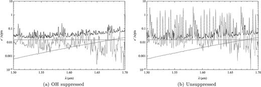
We have measured the level of suppression at each pixel by dividing the control spectrum by the suppressed spectrum (after first correcting the control spectrum for the fact that this is from a single fibre compared to six fibres for the suppressed spectrum); this is shown in Fig. 0008. The mean reduction per pixel between 1.5 and 1.7 μm is ≈17, and the median is ≈1.6. The reduction of the integrated background between 1.5 and 1.7 μm is ≈9.

The background suppression per pixel as a function of wavelength.
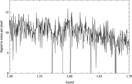
To compare the interline components in the suppressed and control spectra, we first subtract the detector dark current and instrument thermal emission. However, these components are brighter than the interline component we are trying to measure, and the subtraction is inevitably noisy. Fig. 0009 shows a comparison of the electrons per second per pixel due to dark current, thermal emission, and suppressed and unsuppressed OH lines. The statistical fractional error on the suppressed observations is shown in Fig. 0010, which is calculated from the mean and standard deviation of counts per pixel from 15 separate half-hour exposures. The typical error on the interline component is ≈25 per cent; however, there may be unquantified systematic errors on these measurements.
The electrons per pixel per second from the dark current (blue), thermal emission (red) and night sky (grey) compared to the unsubtracted spectra (black) for suppressed and unsuppressed observations. The dark current and thermal emission are significantly brighter than the interline component we are trying to measure.

The fractional error on the counts per pixel for the suppressed sky spectra, calculated as standard deviation/mean, for a half an hour exposure.
Nevertheless, after dark and thermal subtraction, there is no discernible reduction in the background between the OH lines. This is unexpected; the models of Ellis & Bland-Hawthorn () show that if the background (after dark subtraction) is composed of thermal emission, zodiacal scattered light and OH lines, then the interline region should be dominated by light that originates as OH lines, which is scattered by the spectrograph. Thus, suppressing the OH lines should also suppress this light scattered from the OH lines. The fact that we do not see this suggests four possibilities: (i) there is residual instrumental emission which has not been properly removed in the data reduction, (ii) the IRIS2 spectrograph does not scatter significant amount of OH light between the lines, (iii) the interline region is dominated by some source that Ellis & Bland-Hawthorn () did not account for and (iv) the FBGs are not suppressing the OH lines as predicted, and hence the reduction is not as predicted.
We have addressed (i), the possibility of residual thermal emission, as fully as possible in our data-reduction method (Section ). However, we are operating in the regime of very low count rates such that systematic errors may become significant. The raw ADU per pixel in the interline component region is ∼10 in a half-hour exposure, which corresponds to ∼45 e− pixel−1, of which ∼18 e− pixel−1 are due to the sky, and the detector dark current contributes ∼27 e− pixel−1. That is, we are detecting less that 1 e− pixel−1 min−1, and we are dominated by detector noise. At this level, systematics become very important. For example, the effective read noise is ≈8 e− pixel−1, which alone gives ∼15 per cent uncertainty in the interline component measurements. There are systematics in detector linearity as discussed in Section , and there may be other effects such as reciprocity failure (Biesiadzinski et al. ) which are very difficult to characterize.
We can discount (ii) since we have measured the scattering of IRIS2, and indeed it was this empirical scattering model from IRIS2 that was used in the models of Ellis & Bland-Hawthorn (). There is a small change in the PSF of IRIS2 due to a different slit and a different f-ratio at the input; however, this will affect only the Gaussian core of the PSF, and then only slightly, and not at all the Lorentzian wings of the PSF.
Regarding (iii), we have searched for other molecular bands and lines of emission in the H band. We used the SpectralCalc.com facility to compute the emission line intensities from the HITRAN2008 models (High-resolution transmission molecular absorption database; Rothman et al. ). We included lines from H2O, CO2, O3, N2O, CO, CH4, O2, NO, SO2, NO2, NH3, HNO3, N2, HF, HCl, HBr, HI, ClO, OCS, H2CO, HOCl, HCN, CH3Cl, H2O2, C2H2, C2H6, PH3, COF2, SF6, H2S, HCOOH, HO2 and ClONO2. The relative intensities were taken directly from the atmospheric paths of SpectralCalc.com assuming an observing altitude of 1.2 km, a target height of 600 km, standard atmospheric conditions and zenith angle of 0°. The resulting emission is shown in Fig. 0011, where we have normalized the intensity to match roughly the interline component. There are hints that some of the structures in the interline component arise from certain molecular bands. The O2 band at 1.58 μm and a CH4 feature at  m are most obvious, but there are possibly some other broad features due to CO2, N2O and C2H2. However, the relative intensities of these features are not right, and neither is the overall shape of the combined emission from these molecules. Moreover, with the exception of O2 and CH4, there are no features corresponding to the obvious emission lines seen throughout.
The estimated molecular emission from the HITRAN2008 data base (grey) compared to the GNOSIS interline component (black line).
Scattering from aerosols or dust in the upper atmosphere and certain chemical reactions may also produce a nightglow continuum. For example, the continuum produced in the reaction NO + O → NO2 + hν has been found to correlate well with the optical nightglow (Sternberg ; Sternberg & Ingham ), and it has been suggested (Content ) that this may increase in the NIR and is of the same order as the brightness of the interline component measured by Maihara et al. (). We have measured the interline component strength for individual observations as a function of air mass and found no trend; see Fig. 0012. This suggests that the interline component does not have an atmospheric origin, but we caution that the atmospheric emission could be temporally variable, as for the OH lines, which could mask any dependence on air mass. In summary, there are individual features of the interline component due to other atmospheric molecular emission, but as yet we cannot explain the overall structure of the interline emission.
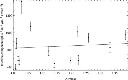
The interline component strength as a function of air mass and the best-fitting linear relation. The error bars show the error on the mean interline component emission.
Finally, we consider (iv) that there may still be unsuppressed OH emission dominating the interline component [e.g. the Q1(3.5) and Q1(4.5) transitions discussed in Section ]. We have tested this and found a weak correlation between the OH line strength and the interline component strength for individual observations [recall that the OH line strength varies by about 10 per cent on the time-scale of minutes (Ramsay et al. ; Frey et al. ) and by a factor of ≈2 throughout the night (Shimazaki & Laird )], shown in Fig. 0013. The r2 goodness of fit is 0.38, with a significance of p < 0.02. Thus, the OH line intensity does indeed affect the interline component. Nota bene, this is expected even with OH suppression and is not an indication that the FBGs are not correctly suppressing the OH lines. Ellis & Bland-Hawthorn () show that at a resolving power of R = 2000, the scattering from residual suppressed OH lines, even though very faint, will still dominate the interline region even after OH suppression. In fact, it is the relative weakness of the correlation between the interline component and OH line strength that must be explained, especially when coupled with the lack of dependence on air mass in Fig. 0012. This will at least in part be due to uncertainty in the measurements. The signal-to-noise ratio on the interline component is poor, and the standard deviation of the residuals to the best fit shown in Fig. 0013 is 160 photons s−1 m−2 arcsec−2 μm−1, which gives an indication as to the error on the interline component measurements. However, the weakness of the correlation may also be a further indication that there is still some unidentified source of interline emission.
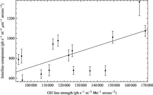
The interline component strength as a function of OH line strength and the best-fitting linear relation. The error bars show the error on the mean interline component emission.
In summary, we feel confident that we can rule out (ii), i.e. we believe we understand the scattering function, but cannot rule out any of the other options. Instrumental artefacts, unknown atmospheric components and inaccurate modelling of the OH lines may all contribute to the interline component at some level.
4.3 Sensitivity
We have measured the sensitivity of GNOSIS with an observation of a low surface brightness galaxy, which obviates the need to address the problem of aperture losses. The galaxy selected was HIZOA J0836−43 (see Cluver et al. ), with an H band surface brightness of 17.3 mag arcsec−2, the details of which were kindly provided by Michelle Cluver. We obtained a half an hour exposure on target, the details of which are given in Table 0002. The resulting spectrum is shown in Fig. 0014 along with a spectrum with no sky or dark subtraction.
The spectrum of the low surface brightness galaxy HIZOA J0836-43 from a half-hour exposure (black), and the same spectrum including the background (grey).
The signal-to-noise ratio per pixel for this observation was calculated by dividing the sky-subtracted spectrum by the square root of the non-subtracted spectrum after first scaling by the detector gain and correcting to the full GNOSIS IFU area (as this spectrum is from only six of the seven IFU elements). The signal-to-noise ratio per pixel is shown in Fig. 0015. The median signal-to-noise ratio per pixel is 10.1. An identical analysis on the control fibre yields an identical median signal-to-noise ratio per pixel. This is because the OH suppression only improves the signal-to-noise ratio near the night-sky lines; between the lines the background is the same, and these interline pixels dominate the calculation of the average signal-to-noise ratio. The improvement that comes from the OH suppression is counteracted by the loss in throughput from the FBG unit. We note that this is not an inherent problem for OH suppression; improvements in throughput of the FBG unit along with lower thermal and detector backgrounds will improve the signal-to-noise ratio. A better understanding of the interline component discussed in Section may also lead to improvements in the suppression of the interline background as proposed in Ellis & Bland-Hawthorn (). We have computed the median signal-to-noise ratio as a function of time and magnitude, which are shown in Fig. 0016.
The signal-to-noise ratio per pixel for the observation of HIZOA J0836-43 shown in Fig. 14.

The median signal-to-noise ratio per pixel as a function of time and magnitude.
4.4 Illustrative observations
We now demonstrate the benefit of OH suppression with three illustrative observations. The first two are of [Fe ii] emission from the Seyfert galaxies and allow a comparison of OH-suppressed and non-OH-suppressed observations. The third is of a candidate L7 dwarf star which is an example of OH-suppressed observation of a continuum source. The purpose of these examples is not to show that GNOSIS is competitive with the current generation of NIR spectrographs. The prototype nature of GNOSIS results in a low overall throughput, a large number of pixels per square arcsecond and resultant high detector noise, and an efficiency loss in having to spend half the exposure time on blank sky, and therefore GNOSIS observations do not give any advantage over standard IRIS2 observations. Rather, we wish to show the potential of OH suppression, by means of a comparison of the OH-suppressed and control spectra. With improvements to the throughput, the thermal background and the detector dark current, similar observations of both emission line and continuum sources will be possible on much fainter objects. We discuss how future instruments can best benefit from the potential of OH suppression and what changes are necessary to do so (Section ).
We give two examples of [Fe ii] emission from the Seyfert galaxies NGC 7674 and NGC 7714. In both cases, we compare a single OH-suppressed fibre to the single control fibre, shown in Fig. 0017. In the case of NGC 7714, the [Fe ii] emission falls between the OH lines and is clearly visible in both suppressed and non-suppressed spectra. In the case of NGC 7674, the [Fe ii] emission falls in a dense region of OH lines, but is still clearly visible in the suppressed spectrum, but less so in the non-suppressed spectrum.
![The [Fe ii] emission from two Seyfert galaxies. The black line is the OH-suppressed spectrum from the middle fibre and the blue is the control fibre. They have been offset for clarity. The red dot marks the expected position of the 1.644 μm [Fe ii] line. The grey lines mark the positions of the brightest OH lines.](https://oup.silverchair-cdn.com/oup/backfile/Content_public/Journal/mnras/425/3/10.1111/j.1365-2966.2012.21602.x/2/m_425-3-1682-fig017.jpeg?Expires=1750475652&Signature=Leu2DwkSPaCl4CBSiyKZl-WQu3kX7vO4CKdR3NC09KwVsMupkJaaviloc5xYscUnhEzRbsSG4Ha7odu3JloEmIVoIk126AMRbbSLybqrUlPhnkuuhWKFJsfG3PQfvs7JPXzkjCro3yRxAhLA0GxS-GbH2f9o-btpKbqT2JH~AstuDlzP4lOasL0WuJyqW0EYGfNQY4pEL5k4a1-rJJhRjtrYUf1SLBoJlJEj8jXex8qIXd5n32yQvMiLBibozyPaBvRA1Z4W~fkjUSLfvpuiPbWqds1ZTrLVdheYFkqeh9ae9bllX8fgS~75tl70xmP2rrVY2fo2WlqfxcSEQwfdow__&Key-Pair-Id=APKAIE5G5CRDK6RD3PGA)
The [Fe ii] emission from two Seyfert galaxies. The black line is the OH-suppressed spectrum from the middle fibre and the blue is the control fibre. They have been offset for clarity. The red dot marks the expected position of the 1.644 μm [Fe ii] line. The grey lines mark the positions of the brightest OH lines.
Fig. 0018 shows a GNOSIS spectrum of a candidate L7 dwarf, 2MASS J0257−3105, which was observed as part of Professor C. Tinney's scheduled GNOSIS observation on 2011 November 27 (see Table 0002). For these observations no control fibre was used, and therefore no comparison of OH suppressed spectra to non-suppressed can be made. However, our experience observing brown dwarfs with IRIS2 tells us that the spectrum is comparable in quality and signal-to-noise ratio to standard long-slit IRIS2 spectroscopy. The observations provide an example of the kind of science which may be done with OH suppression on continuum sources. The object was selected as an L7 dwarf from Kirkpatrick et al. (). However, a comparison of the H-band spectrum with standard spectra from Burgasser et al. () shows that it has stronger CH4 absorption, similar to an early T dwarf. An exact spectral type is difficult to give since none of the standard spectra gives a perfect match.
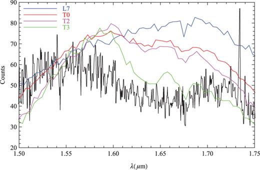
A GNOSIS spectrum of an L7 dwarf from Kirkpatrick et al. (2008) compared to standard star spectra from Burgasser et al. (2004). The H-band spectrum shows stronger CH4 absorption than expected for an L dwarf.
5 DISCUSSION
We have demonstrated the first instrument to employ OH suppression with FBGs. To test the performance of this new technology, we made five key measurements: (i) the overall, and component, instrument throughput, (ii) the instrument sensitivity, (iii) the level of OH suppression, (iv) the interline component and (iv) illustrative observations of Seyfert galaxies. We now discuss the results of these measurements in the context of the continuing development of OH-suppressed NIR spectrographs.
The total throughput is ≈4 per cent but the throughput of IRIS2 is only ≈12 per cent while that of GNOSIS itself is ≈36 per cent. The latter can be greatly improved by the following measures. First, on a specialized OH suppression spectrograph, the need for relay optics could be eliminated by using a fibre vacuum feed-through. This would remove at least four optical surfaces, greatly improve alignment losses and have the additional benefit of lowering the thermal background. Secondly, an even larger improvement could be made in the photonic lanterns. Recent laboratory tests imply that the efficiency of the photonic lanterns is a function of the input f ratio, and that by feeding the lanterns at a slower speed we could increase the efficiency from 50 to ≈70 per cent. These tests are preliminary but indicate that the coupling efficiency of the lanterns may depend on the mode being coupled.
The sensitivity of GNOSIS+IRIS2 is about that of IRIS2 when used in its standard spectrograph mode with a slit. That is, in the particular implementation used for GNOSIS, the benefits of OH suppression are offset by lower throughput, higher detector background, higher thermal background and lower observing efficiency. The low throughput has been discussed above and in Section .
The high detector background comes from the fact that a small field of view of 1.2 arcsec is being divided into seven elements, and the spectra from each of these are being sampled by ≈2 pixels; thus, when extracting the spectra for each spectral pixel, there is dark current and read noise from ≈14 spatial pixels, compared to ≈2 spatial pixels for the same sky area using IRIS2 (recall that GNOSIS feeds IRIS2 at a slower f ratio than for long-slit IRIS2 observations). Since the background is dominated by the detector dark current, this is a significant loss of sensitivity.
The high thermal background results almost entirely from the slit block and is a significant source of noise at
 m. GNOSIS observations are also less efficient than IRIS2 observations in that half the time must be spent on the sky, whereas with IRIS2 the object can be nodded up and down the slit. Note that these problems are not intrinsic to OH suppression in general, and it is easy to envisage improved instruments that circumvent all these issues.
Using photonic lanterns with a larger number of cores will allow the use of larger diameter fibres and thus increase the field of view per fibre, thereby lessening the effects of detector background. This will require faster spectrograph optics of around ≈f/2.8.
The low observing efficiency is simply a matter of cost. If two IFUs can be afforded, then cross-beam switching of observations will ensure that all observing time is spent on target.
Of course, there are also many improvements that should be made to the spectrograph itself to improve the overall efficiency. For example, newer detectors with lower dark current and higher quantum efficiency, volume phase holographic (VPH) gratings instead of grisms and fixed format optics will all improve the throughput. These improvements would of course be true of non-OH suppressed spectrographs as well.
The suppression of the OH lines was a success. The sky spectra and the object spectra show that the OH lines can be cleanly removed whilst maintaining good throughput (in the FBGs themselves) between the lines. The level of suppression is high with ≈78 per cent of the targeted lines suppressed at the required level. Of the lines which do not meet the required level of suppression, 37 per cent are due to residuals from the Q1(3.5) and Q1(4.5) OH lines (Section ). Similarly, there is an unsuppressed O2 line.
The expected reduction of the interline component was not observed. This seems to indicate either an unaccounted source of interline emission, inaccuracy of our OH line models or unaccounted-for systematic errors.
Systematic errors are a real possibility since we are operating in a very low count regime of less than 1 e− pixel−1 min−1, and we are dominated by detector noise. We have observed (and corrected for) systematic deviations from detector linearity as discussed in Section and have noted that there may still be other effects such as reciprocity failure (Biesiadzinski et al. ) which are very difficult to characterize.
We have already noted that specific transitions in the OH energy levels were not properly suppressed, which seems to be due to a larger energy gap between the Λ doublets than predicted in our models. It is possible that other such errors may exist in fainter lines, or that other branches of lines are brighter than supposed, but we are unable to measure this with the current sensitivity. Unsuppressed faint OH lines could masquerade as continuum due to the spectrograph scattering.
On the other hand, there could be emission from another source. A thorough search of the emission lines from 33 different molecules in the HITRAN2008 data base cannot account for the structure and the faint lines we observe in the interline component except for a couple of individual features from O2 and CH4. Also there is no dependence of the interline component on air mass, as would be expected for an atmospheric source. However, there always remains the possibility that there is another overlooked source or that relative intensities of the molecular emission need improvement.
In order to try to distinguish between these two possibilities, we looked at the correlation between the interline component and the OH line strength, and found that they were only weakly correlated. If true, this suggests that there is indeed an unknown source of interline emission, since otherwise the correlation would be much stronger. However, this interpretation should be treated with much caution due to the large measurement errors and possibly significant systematic errors on the interline measurements.
The absolute level of the interline emission is 860 ± 210 photons s−1 m−2 arcsec−2 μm−1which is slightly higher than that measured by Maihara et al. (, 590 photons s−1 m−2 arcsec−2 μm−1) and slightly less than that measured by Cuby, Lidman & Moutou (, 1200 photons s−1 m−2 arcsec−2 μm−1). We again point out that there may be significant systematic error on our measurement due to the low count rates measured. However, the similarity to previous measurements could indicate that we have indeed reached a floor in the interline component which is significantly higher than the zodiacal scattered light background (see Ellis & Bland-Hawthorn ).
If the interline emission is the result of unsuppressed OH lines due to inaccuracies in our OH line models, this may be fixed with better models or with wider FBG notches to account for such uncertainties. However, as things stand, the lack of a reduction in the interline component suggests that OH suppression will find its niche in low-resolution (R ≲ 3000) observations which would normally be insufficient to ‘resolve out’ the OH lines. Indeed, OH suppression could be used at low resolutions, R ∼ 500, at which conventional observations would be impractical.
The suggested benefit of OH suppression at low resolution is supported by our observations of Seyfert galaxies (Section ). We find that in regions where the OH line density is high, as for NGC 7674, the low resolution of IRIS2 makes it difficult to identify the [Fe ii] emission in the control spectrum, but that the line is obvious in the suppressed spectrum. Similarly, when working between the lines as for NGC 7714, the benefits of OH suppression are much less apparent since in this case we are limited by the detector dark current in both cases.
We conclude by noting that GNOSIS is the first step towards an OH-suppression-optimized spectrograph, and not a full-fledged facility instrument. The overall performance of the OH suppression unit itself is good but can be substantially improved. However, there remains uncertainty about the origin of the interline emission, which could be higher than predicted either due to some unknown source of emission or because of unaccounted-for systematics in the detector. The next step will be to design and build a spectrograph optimized for an FBG feed, which will avoid the disadvantages that result from retrofitting an OH suppression system to an existing spectrograph. Furthermore, in doing so we can capitalize on the lessons learnt with GNOSIS in terms of detector background, optimal spectral resolution and design.
ACKNOWLEDGMENTS
We thank Pierre Rousselot and Chris Lidman for illuminating discussions on the OH spectrum. We also thank Michelle Cluver for kindly providing the details of HIZOA J0836−43 for observation. We thank the referee for useful comments which have improved this paper. GNOSIS was funded by an ARC LIEF grant LE100100164. This research has benefited from the SpeX Prism Spectral Libraries, maintained by Adam Burgasser at http://pono.ucsd.edu/~adam/browndwarfs/spexprism.
References
