Regularization techniques for PSF-matching kernels - I. Choice of kernel basis Free

Abstract

Introduction

Studies of variability in astronomy typically use image subtraction techniques in order to characterize the magnitude and type of the variability. This practice involves subtracting a prior-epoch [generally high signal-to-noise (S/N)] template image from a recent science image; any flux remaining in their difference may be attributed to phenomena that have varied in the interim. This technique is sensitive to both photometric and astrometric variability and can uncover variability of both point sources (such as stars or supernovae; e.g. Sako et al. ; Udalski et al. ) and extended sources (such as comets or light echoes; e.g. Newman & Rest ). Successful application of this technique shows that it is sensitive to variability at the Poisson noise limit in a variety of astrophysical conditions (Alard & Lupton ; Alard ; Bramich ; Kerins et al. ) and in this regard may be considered optimal.

There are several reasons for preferring such an approach over catalogue-based searches. First, many types of variability are found in confused regions of the sky, and it may be difficult to deblend the time-variable signal from the non-temporally-variable surrounding area. This is particularly true for supernovae and active galactic nuclei, which are typically blended with light from their host galaxies. However, such confusion is not limited to stationary objects. Moving Solar system bodies may serendipitously yield false brightness enhancements in the measurement of a background object if the impact parameter is small compared to the image's point spread function (PSF). For this reason, removal of non-variable objects is preferred before attempting to characterize variable sources in images.

Image subtraction is also an efficient technique as the vast majority of pixels in an image do not contain signatures of astrophysical variability. Any pixel-level analysis of a difference image will, therefore, be restricted to those sources that are temporally variable (as opposed to analysing all sources within an image). While many variants of this technique have been published (Tomaney & Crotts ; Alard & Lupton ; Bramich ; Albrow et al. ) and many versions implemented in automated variability-detection pipelines (Bond et al. ; Rest et al. ; Darnley et al. ; Miller, Pennypacker & White ; Udalski et al. ), there does remain room for improvement in the robustness of the image subtraction and in the reduction of subtraction artefacts. We refer the reader to Wozniak () for an in-depth summary on the practical application of these image subtraction techniques.

Image subtraction

In image subtraction we assume that we have two images of the same portion of the sky, taken at different epochs, but in the same filter. We will call the image that contains the variability of interest the ‘science’ image and the template image to be subtracted the ‘reference’ image. The images will, in general, be astrometrically misaligned, but this can be resolved by using sinc-based image registration methods that preserve the noise properties of the original image. In practice, windowed sinc functions are used that do introduce covariance between the pixels; there is a direct trade-off between the size of the warping kernel and the degree of correlation after registration (the correlation trends to zero as the window becomes infinite in extent). After astrometric alignment, a given astrophysical object will be represented in the reference image as a sub-array of pixels R(x, y) and in the science image as S(x, y), with the same span in x and y. Each image will, however, have a different PSF, which is the spatial response of a point source due to the atmosphere, telescope optics and instrumental signatures. PSF matching of the images is required before we can subtract one image from the other and is the essence of the image subtraction technique.

PSF MATCHING

We typically assume that the reference image is a high-S/N representation of the field, for example an image co-add made through a mosaicking process, or a single image taken on a night with particularly good seeing. A standard assumption (e.g. Alard & Lupton ; Alard ) is that S(x, y) can be modelled as a convolution of R(x, y) by a single PSF-matching kernel K(u, v), with an additional noise component ε(x, y);

Our goal in this paper is to develop an effective method for determining K(u, v).

Linear modelling of K(u, v)

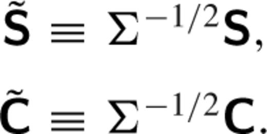
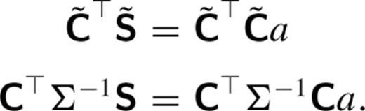
As inputs to the PSF-matching technique, we assume that images are astrometrically registered and background subtracted (while the latter constraint is not a necessity, it does enable us to restrict our analysis here to the respective shapes of the PSFs). To proceed, we make the assumption that K(u, v) may be modelled as a linear combination of basis functions K_i(u, v), such that K(u, v) = ∑_ia_iK_i
(u, v) (Alard & Lupton ). The basis components do not have to be orthonormal, nor does the basis need to be complete (indeed, it may be overcomplete). However, it is desirable to choose a shape set that compactly describes K(u, v), such that the number of required terms is small.

By formulating the kernel decomposition as a linear expansion, we may recast equation as the vectorized equation

where C is the matrix of functions C_i ≡ (K_i ⊗ R) evaluated at each pixel. For any given kernel basis set, the goal is to find the coefficients a_i associated with each K_i.

We proceed using standard linear least-squares analysis. We assume that the noise is uncorrelated and known; ε is therefore the product of a diagonal matrix (which must exist as covariance matrices are positive definite and hence invertible) we obtain the modified equation

which is just another linear model, now with the error term Z having the identity matrix for the covariance. This reduces to the weighted linear least-squares equation

with

 The normal equations for estimating a are

This may be cast in the familiar form of b = M a with

In discrete pixel coordinates, this corresponds to

where σ²(x, y) represents the known variance per pixel. The creation of the matrices M_ij and b_i therefore requires a convolution of the reference image with each basis kernel.

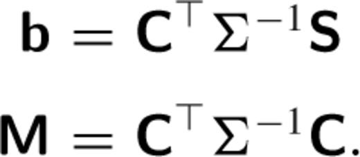
The least-squares estimate for a is . A difference image is then constructed as . Because the estimate of is explicitly dependent on both S(x, y) and R(x, y), the residuals in the difference image may not necessarily follow a normal distribution¹, with σ² ≠ 1 due to this covariance. The residuals should however have a flat power spectral density.

Invertability of

When a large set of basis functions is used, the matrix may be ill-conditioned or even singular. This can be quantified by the ‘condition number’ of M, which we define as the ratio of the largest to the smallest eigenvalues. When the condition number is large, inversion of M will be numerically unstable or infeasible.

A common approach when trying to invert an ill-conditioned matrix is to compute instead a pseudo-inverse, or an approximation to one in which eigenvalues that are numerically small are zeroed out. As M is symmetric, we can decompose it as with V an orthogonal matrix and with eigenvalues d₁ ≥ d₂ ≥ ⋅⋅⋅ ≥ d_n ≥ 0. We define to be a truncation of D where d₁/d_{i + 1} becomes too large. Then, we define the pseudo-inverse of D_i as . Note that this allows for the definition of a pseudo-inverse of M as . Analogous to D_i, define ssV_i to be the same as the matrix V_i in the first i columns and zero elsewhere. Typically this truncation threshold is defined by the machine precision of the computation (e.g. for double-valued calculations, ). However, significantly larger limits for d_min may be used to avoid underconstrained parameters, such as in Section .

SUM-OF-GAUSSIAN BASES

The original PSF-matching bases proposed by Alard & Lupton () and Alard () (referred to here as ‘Alard–Lupton’ or AL bases) used a sum of multiple Gaussians, each modified by a two-dimensional polynomial:

where the index i runs over all permutations of n, p, q. This basis set effectively uses n = 1, … , N Gaussian components, each with width σ_n, and each modified by a set of Gauss–Hermite polynomials (e.g. Wnsche ) expanded out to order O_n (0 ≤ p + q ≤ O_n). The total number of basis functions in the set is ∑_n(O_n + 1) × (O_n + 2)/2.

The number N and width σ_n of the Gaussians, as well as spatial order of the polynomials O_n, are configurable but are not fitted parameters in the linear least-squares minimization. Therefore these are tuning parameters of the model. Typically, a priori information such as the widths of the image PSFs is used to choose these values (e.g. Israel, Hessman & Schuh ). In a representative implementation (Smith et al. ), three Gaussians are used, with the narrowest Gaussian expanded out to order 6, the middle to order 4 and the widest to order 2. This leads to a total of 49 basis functions used in the kernel expansion.

The practical application of this algorithm has been very successful, and it has been used by various time-domain surveys such as MACHO (Alcock et al. ), OGLE (Wozniak ; Udalski et al. ), MOA (Bond et al. ), SuperMACHO (Smith et al. ; Rest et al. ), the Deep Lens Survey (Becker et al. ), ESSENCE (Miknaitis et al. ), the SDSS-II Supernova Survey (Sako et al. ) and most recently analysis of commissioning data from Pan-STARRS (Botticella et al. ).

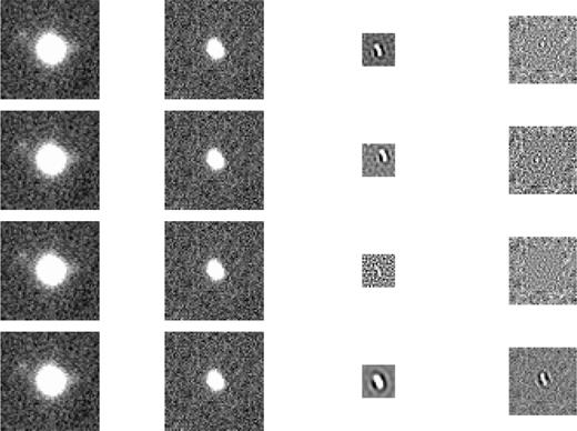
The top row of Fig. ¹ shows an instance of successful PSF matching using this sum-of-Gaussians basis. The first column represents a high-S/N image of a star R(x, y) generated from an image co-addition process applied to data from the Canada–France–Hawaii Telescope (CFHT). The second column shows this same star, aligned with the template image to sub-pixel accuracy, in a single science image S(x, y). The star is obviously asymmetric, potentially due to optical distortions such as focus or astigmatism, or due to tracking problems during acquisition of the image. The PSF-matching kernel thus will need to take the symmetric R(x, y) and elongate it along a vector oriented approximately 135° from horizontal. The first row, third column shows the best-fit PSF-matching kernel using N = 3 Gaussians with σ_n = [0.75, 1.5, 3.0] pixels and each modified by Hermite polynomials of the order of O_n = [4, 3, 2], respectively. The total number of terms in the expansion is 31. The first row, right column shows the resulting difference image D(x, y). The subtraction is obviously very good, with the remaining pixels described by a distribution.

Figure 1

Difference imaging results when using a sum-of-Gaussian basis. The first column shows the reference image to be convolved R(x, y), the second shows the science image S(x, y) the reference is matched to, the third column shows the best-fit 19 × 19 pixel PSF-matching kernel K(u, v) and the fourth column shows the resulting difference image D(x, y). Row 1: results when using a basis set with σ_n = [0.75, 1.5, 3.0] pixels, O_n = [4, 3, 2]. Row 2: results when the images are misregistered by 3 pixels in both coordinates, requiring significant off-centre power in the kernel. Row 3: results when the basis Gaussians are too large compared to the actual PSF-matching kernel (σ_n = [3.0, 5.0] pixels, O_n = [3, 2]). Row 4: results when the polynomial expansion is not carried to high enough order (σ_n = [0.75, 1.5, 3.0] pixels, O_n = [1, 1, 1]).

Open in new tabDownload slide

Limitations of the model

The intrinsic symmetries of Hermite polynomials (symmetric for even order, anti-symmetric for odd order) mean that the Gauss–Hermite bases possess a high degree of symmetry about the central pixel. This makes it difficult to concentrate the kernel power off-centre when using an incomplete basis expansion. Such functionality is necessary when the flux needs to be redistributed on the scale of the kernel size, such as when there are astrometric misalignments. While it is possible to compensate for misalignment using kernels derived from this basis, this requires concentrating the kernel strength in the high-order terms. There are practical limitations to the efficacy of this including the scale and orientation of the required shift and the number of basis terms used.

As a concrete example, the second row in Fig. ¹ shows the best-fit kernel derived when there is a 3-pixel shift in both the x and y directions. The kernel needs to have power in the first quadrant (upper-right) at the scale of 3 pixels. The image of the kernel (third column) shows that while it is obviously able to do so, the matching suffers in the third quadrant, as the difference image shows obvious residuals. These pixels result in an unacceptable distribution; recall that we were able to yield σ² = 1.01 for well-registered images (top row).

Another limitation of the model is that there are a variety of tuning parameters. This includes the number of Gaussians in the basis, their widths and their spatial orders. These parameters are typically chosen using a set of heuristics. If there is a mismatch compared to the true underlying kernel, this process will fail. The third row of Fig. ¹ shows PSF-matching results when the basis Gaussians are too big and are unable to reproduce the small-scale differences in the PSFs. This yields obvious residuals in the difference image, which follow a distribution. The fourth row of Fig. ¹ shows results when the Gauss–Hermite polynomials are not allowed to vary to high enough order, also yielding unacceptable residuals in the difference image.

Clearly the results of this process are sensitive to the choice of several tuning parameters, which makes this difficult to implement robustly. In a statistical sense, selection of tuning parameters (which includes selecting the number of basis functions used) usually has a much larger effect on performance than does the choice of basis functions. A process that results in a reduction in the number of kernel tuning parameters, while maintaining the quality of the difference images, would greatly improve the effectiveness of this method.

DELTA-FUNCTION BASES

The most general technique for modelling K(u, v) is to use a ‘shape-free’ basis, which consists of a delta-function at each kernel pixel index: K_ij(u, v) = δ(u − i)δ(v − j). A kernel of size 19 × 19 will then have 361 orthonormal, single-pixel bases. In this situation there are no tuning parameters, which is an obvious benefit. However, in any choice of basis there is a trade-off between flexibility in the forms the fitted function can take and variability in the resulting fit (the so-called ‘bias-variance’ trade-off). The delta-function basis provides complete flexibility, and as such can account for features such as arbitrary off-centre power required to compensate for astrometric misregistration (e.g. Bramich ). But to avoid gross overfitting, that flexibility needs to be tempered to keep the variance in check.

Fig. ² shows the results of PSF matching using such a basis, using the same objects as in Fig. ¹. The top row demonstrates the results for exactly aligned images, while the bottom row demonstrates the results for images misaligned by 3 pixels in both x and y. The difference images are qualitatively similar. However, the best-fit solutions obviously yield large variations within the kernels themselves, and do not match expectations of what the actual kernel should look like. The reason for this can be found in the distribution of pixels residuals in the difference image. Both images follow a distribution. This indicates that the residuals have lower variance than Gaussian statistics would suggest. Indeed, in Fig. ², column 4, the residuals appear smoother than random noise. This is impossible unless we have overestimated the variance in our images, or unless the kernels themselves are removing some fraction of the noise.

Figure 2

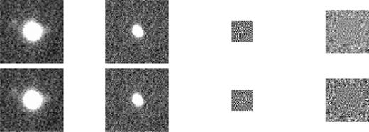
Difference imaging results when using a delta-function basis. Columns are the same as in Fig. 1. Row 1: results when using an unregularized delta-function basis. Row 2: results when the images are misregistered by 3 pixels in both coordinates.

Open in new tabDownload slide

The large numbers of basis shapes (361 degrees of freedom versus 31 for the sum-of-Gaussians) make it highly likely that we are overfitting the problem. The kernel thus has the ability to match both the underlying signal and the associated noise in the two images. So while this technique is optimal for matching pixels in two images – where those pixels are a combination of signal and noise – it is not necessarily optimal for uncovering the true PSF-matching kernel.

Current codes that use digital kernels (Bramich ; Albrow et al. ) are able to achieve relatively noise-free representations of the matching kernel by using all pixels in the image as constraints on K(u, v). Importantly, this technique has been generalized to allow construction of a spatial model of the kernel K(u, v, x, y), which must vary across an image due to spatial variation in the underlying PSF fields (e.g. Quinn, Clocchiatti & Hamuy ). In practice, these spatial models enable interpolation of the matching kernel at all locations in an image, using fitted kernels at particular locations as constraints on the global model.

In this context, one consequence of the overfitting is that the PSF-matching kernel derived for any given object may not be directly applied to neighbouring objects, since the solution is significantly driven by the local noise properties. These types of high variance estimators are particularly poor as inputs to interpolation routines, or as constraints on the spatial model of the kernel K(u, v, x, y). Below, we explore how introducing a certain amount of bias into this estimator can improve its performance.

DELTA-FUNCTION BASES WITH REGULARIZATION

The delta-function basis can flexibly fit a kernel of any form, but as we have shown, this flexibility is both its strength and weakness. As is, the method significantly overfits, absorbing substantial noise fluctuations into the fit and thus giving estimated kernels with excessive variance. A solution is to introduce some amount of bias into the fit to reduce the solution variance by a much larger factor [if ‘bias’ sounds pejorative, note that this is just a kind of smoothing; we note that digital kernel codes of Bramich () and Albrow et al. () achieve a degree of smoothing by using binned pixels in the outer portions of the kernels]. When fitting a smooth function such as K(u, v, x, y), we prefer fitted kernels for which nearby solutions do not vary too greatly. This bias will enable such a fit with vastly reduced mean-squared error.

Among the various approaches to dealing with overfitting, the most common are through linear regularization techniques (e.g. section 18.5; Press et al. ). Using these, we may penalize undesirable features of the fit, usually by adding a penalty term to our optimization criterion. For instance, when fitting a smooth function, we want to penalize fits f that are too rough or irregular. One way to do this is to add to the least-squares objective a term penalizing the second derivative, λ · ∫|f′′(x)|²dx. Here, the scaling factor λ is a tuning parameter that determines the balance between fidelity to the data and the desired smoothness. In the case of kernel matching, we may extend this idea with a two-dimensional penalty that approximates λ · ∫∫|∇f(x, y)|² dx dy.

The one-dimensional second derivative of a function f around pixel x may be approximated using the central finite difference f′′(x) ≈ f(x − 1) − 2f(x) + f(x + 1). Since the delta-function bases have unit height and no intrinsic shape, regularizing the coefficients a_i is equivalent to regularizing the shape of the resulting kernel (care must be taken to apply the regularization penalty to only those pixels that are associated spatially). In matrix terms, this one-dimensional regularization may be represented by R₁a, with

which is of dimension (m − 2) × m, where m here is the total number of pixels in the kernel². A generalization of this to two dimensions results in a five-point stencil that sums the local derivative along both axes, f′′(x, y) ≈ f(x − 1, y) + f(x + 1, y) + f(x, y − 1) + f(x, y + 1) − 4f(x, y), with an associated matrix R₂.

The finite calculation of this penalty is implemented through the matrix equations

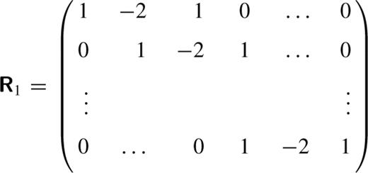
where a represents the amplitude of each delta function, and R₂ encapsulates the coefficients that approximate the local second derivative of the resulting kernel. We define the matrix , which makes the second derivative penalty . This matrix is used to regularize the normal equations (equation ) with strength λ,

Note the similarity to equation , with the only difference being . Here λ represents the strength of the regularization penalty, and is the sole tuning parameter in this model.

Fig. ³ shows results for the same set of objects displayed in Figs ¹ and ², but using regularization of the delta-function basis set. The top row shows the results for aligned images, and λ = 1. Note that the kernel looks very much as anticipated, being compact and having a shape aligned approximately 135° from horizontal. Residuals in the difference image follow a distribution. The second row shows the results when the images are misaligned by 3 pixels in x and y. The kernel merely appears shifted by the same amount compared to the aligned images, and the difference image follows a quantitatively similar distribution. This effectively demonstrates that this method can reproduce kernels with off-centre power. The third row shows the results with λ = 0.01; the shape of the PSF-matching component of the kernel is just barely discernible above its noise, suggesting that the regularization is too weak. The difference image is, however, acceptable []. The fourth row shows the results with λ = 100. The kernel is far smoother than in previous runs. However, this appears to be at the expense of residuals in the difference image, which follow a distribution. This suggests that too much weight has been given the smoothness of the kernel compared to the residuals in the difference image, indicating that the regularization is too strong. The general trend is that with increasing lambda, the variance in the difference image increases. The noise properties of the difference image evolve from being too smooth, to approximately white in spectrum, to having residual features at a similar scale as the kernel.

Figure 3

Difference imaging results when using a regularized delta-function basis. Columns are the same as in Fig. 1. Row 1: results when using a regularized delta-function basis with λ = 1.0. Row 2: results when the images are misregistered by 3 pixels in both coordinates, λ = 1.0. Row 3: results using ‘weak’ regularization of the kernel, with λ = 0.01. Row 4: results using ‘strong’ regularization of the kernel, with λ = 100.

Open in new tabDownload slide

Overall, this technique appears very effective. We are able to create general, compact kernels that represent the underlying shape of the PSF-matching kernel with only one tuning parameter, the strength of the regularization λ. The role of λ is effectively to exchange variance in the resulting difference image with variance in the kernel itself. By increasing the value of λ, we are able to smooth the kernel while increasing the variance in the difference image. We explore various methods to establish the optimal value of λ below.

Choice of tuning parameter »

Choosing a good tuning parameter is essential for good performance of a regularization method. If λ is too high, the fit will be too smooth (high bias, low variance); if λ is too low, the fit will be too rough (low bias, high variance). The goal of data-driven methods for choosing tuning parameters is to find the sweet spot in the bias-variance trade-off. While choosing a good value for λ is a hard statistical problem, there are a variety of methods that have proven successful in practice. These methods construct a statistical estimate of mean-squared error and choose λ to minimize it. For instance in cross-validation (reviewed in Kohavi ), the data set is broken into pieces, and each piece is left out in turn during the fit. The (prediction) mean-squared error is derived from the average-squared error of the fits in predicting the part of the data that was left out. Another approach, called empirical risk estimation (Stein ), uses the data themselves to compute an (unbiased) estimate of original fit's mean-squared error and chooses λ to minimize it. The theoretical justification for these methods is that, when properly done and with sufficiently large data sets, the chosen λ is close to the value that minimizes the corresponding mean-squared error function.

A second tuning consideration is that frequently a set of fitted kernels will be used to constrain a spatial model K(u, v, x, y) that will be applied to all pixels in an image. Therefore we must give a large weight to our ability to interpolate between the ensemble of kernel realizations used to constrain K(u, v, x, y). One metric for this is to examine the predictive power of a kernel derived from one object, and applied to a neighbouring object. At small separations, the quality of each difference image should be similar, indicating that the initial solution was not significantly driven by the local noise properties.

We explore the practical application of these ideas below using several sets of CCD images from the CFHT plus Megacam imager, calibrated using the ELIXIR pipeline of Magnier & Cuillandre (). The template image used is the median of several images into a single high-S/N representation of the field. The variance per pixel is determined from the image pixel values divided by the gain.

Empirical risk estimation

We first construct a loss function that represents the sum of squared differences between the true (unknown) kernel coefficients a and , which is our estimate of the kernel coefficients when the tuning parameter is set to the value λ:

The expectation value of is the statistical risk we will minimize through our choice of λ³. When M is well conditioned, we can construct an unbiased estimator of the true risk as (section 2, Stein )

 We note that this estimator of risk does not require tuning parameters. If we let be the minimizer of R, then we choose as the estimate of a.

For the circumstance that M is ill-conditioned, we present an adjustment to R from equation . Following the notation from Section , for any i define . This corresponds to being a projection matrix on to the space of the eigenvectors of M that correspond to its i largest eigenvalues. Note that i is now an additional tuning parameter, corresponding to the choice of condition number (denoted by symbol Λ) for matrix M (Section ). A biased estimate of the statistical risk is then

While introducing bias into the estimator of statistical risk seems bad, it can be necessary in situations where M is ill-conditioned. Small eigenvalues of M correspond to there being very little information along the associated eigenvectors. By zeroing out these eigenvalues we are effectively saying we cannot reliably estimate with this little amount of information. Hence, we concentrate on getting the estimation correct on the eigenvectors with larger eigenvalues.

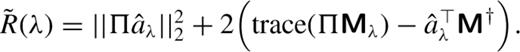
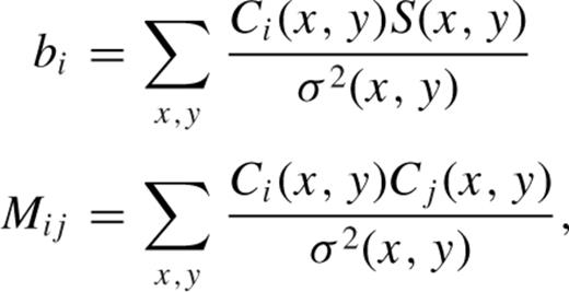
For each object detected in the CFHT images, and for given values of the condition number Λ in the range 4 ≤ log (Λ) < 6, we evaluate R(λ) at values of −2 ≤ log (λ) < 2. Fig. ⁴ shows a typical outcome of this analysis for a single object. Along the y-axis we show the associated value of the conditioning parameter Λ, and along the x-axis the value of λ at which R(λ) is evaluated. The solid line shows the minimum value of R(λ) for each Λ.

Figure 4

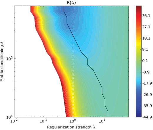
Values of the empirical risk R(λ), as defined in equation (14), for different values of the matrix conditioning parameter Λ, and the regularization strength λ. At all Λ, we determine the minimum values of R(λ), which are connected by the solid black line. The dotted vertical line represents the fiducial value of λ = 1. The global minimum of R(λ) is realized with minimal matrix conditioning and at a value of λ = 0.5.

Open in new tabDownload slide

We note that as we decrease the acceptable matrix condition number, thereby truncating more eigenvalues from the matrix pseudoinverse, the optimum value of λ increases. For matrices with effectively no conditioning (large Λ), the optimal value of λ is near λ = 0.5. This is in fact the global minimum of the risk. A similar result is obtained by looking at all objects within an image and summing their cumulative risk surfaces. We regard λ = 0.5 as the value preferred by the empirical risk estimation technique, with a range of nearly-equivalent risk in the range 0.3 < λ < 1.0.

Predictive ability

In most PSF-matching implementations, several dozen objects across a pair of registered images are used to create individual K(u, v); ideally these should evenly sample the spatial extent of the images. Due to spatial variation in the PSFs of the images, caused by optical aberrations or bulk atmospheric effects, the single kernel that PSF-matches all objects in an image must itself vary spatially. In this case each of the kernels K(u, v) is used to build the spatially varying PSF-matching kernel K(u, v, x, y). This is typically implemented as a spatial variation on the kernel coefficients K(u, v, x, y) = ∑_ia_i(x, y)K_i(u, v). This assumption of a slowly varying underlying kernel suggests a new metric for consideration: the quality of the subtraction for data that were not used in the kernel fit. This predictive ability is quantified below by comparing the subtractions of neighbouring stars with each other's kernels.

In all CFHT images, we identify object pairs separated by more than 5 pixels but less than 50, a range of separations where we expect the intrinsic spatial variation of the underlying kernel to be minimal. The kernel derived for each object in a pair is applied to its complement, and the quality of each difference image assessed. For components A and B of each object pair, this yields difference image D_AA which is the difference image of object A with kernel A, D_AB which is the difference image of object A with kernel B and analogous images D_BA and D_BB. We assess the quality of each difference image using the width of the pixel distribution normalized by the noise, defined as e.g. σ_AA, within the central 7 × 7 pixels of the difference image. While we do not expect this distribution to have a width of exactly 1.0 due to the covariance between the solution and the input images, we do desire that the quality of D_AB and D_BA should not be significantly worse than that of D_AA and D_BB.

We aggregate the ‘even’ statistics σ_AA and σ_BB into distribution Σ_E and the ‘odd’ statistics (σ_AB, σ_BA) into Σ_O. We further examine the distribution of , which is created from all measurements of and . This statistic reflects the deterioration in an object's difference image when using a counterpart's kernel, compared to the optimal kernel derived for that object.

We plot the distributions of these values in Fig. ⁵. The top panel provides the median values of these distributions for the sum-of-Gaussian (AL) basis (left), for the unregularized delta function basis (λ = 0; centre) and for delta-function regularization strengths of −2 < log (λ) < 2 (right). The bottom panel plots the effective standard deviation of the distribution, defined as 74 per cent of the interquartile range.

Figure 5

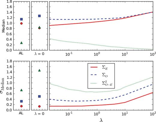
Median statistics assessing the predictive ability of different kernel bases. The top panel shows the median values of statistics Σ_E (red circle and solid line), Σ_O (blue square and dashed line) and Σ²_O-E (green triangle and dotted line) for ‘Alard–Lupton’ (AL) bases, for delta-function bases with λ = 0 and then for a range of −2 < log (λ) < 2. All statistics are defined in Section 5.1.2. The bottom panel shows the standard deviation of the distribution, defined as 74 per cent of the interquartile range.

Open in new tabDownload slide

The lowest median residual variance Σ_E comes from difference images made using an unregularized λ = 0 basis, the reasons for which we have examined in detail in Section . However, as expected the predictive ability of this basis is by far the worst, having the highest median , as well as large variance within this distribution. As we ramp up the regularization strength, the predictive ability of the kernels increases (low ), but at the expense of the quality of the difference image itself (large Σ_E).

To find an acceptable medium between these two considerations, we will use the results from the sum-of-Gaussian (AL) basis as a benchmark, since it has been shown to produce effective spatial models (Section ). For the AL basis, the median values of Σ_E, Σ_O and are 0.99, 1.14 and 0.28, respectively. Similar results are obtained with delta-function regularization strengths of λ ≈ 0.2, 0.7 and 0.2. For AL the σ_median values of Σ_E, Σ_O and are 0.14, 0.33 and 0.74, respectively. These are matched (or bested) in the regularized basis for λ ≤ 0.2, λ = 0.2 and 0.2 ≤ λ ≤ 6, respectively.

In summary, using delta-function regularization strengths of λ ≈ 0.2, we are able to achieve difference images with a similar quality to those yielded by the sum-of-Gaussian AL basis (using Σ_E as our metric). These models have similar predictive ability when applied to neighbouring objects (quantified using Σ_O and ), making them useful for full-image spatial modelling. Finally, they are seen to be generally applicable, having a small variance in the above statistics when evaluated over several hundreds of object pairs.

Conclusions

We have examined here the choice of basis set on the quality of PSF-matching kernels and their resulting difference images. These include the traditional sum-of-Gaussian (AL) basis and a digital basis based upon delta-functions. We find that while the delta-function kernels are the most expressive, they are also the least compact in terms of localization of power within the kernel. Having one basis component per pixel in the kernel, they tend to overfit the data and are more sensitive to the noise in the images instead of the intrinsic PSF-matching signal.

We introduce a new technique of linear regularization to impose smoothness on these delta-function kernels, at the expense of slightly higher noise in the difference images. These regularized shapes are shown to be flexible and yield solutions with sufficient predictive power to prove useful for spatial interpolation. We outline two methods to determine the strength of this regularization that minimize the statistical risk of the kernel estimate and examine the predictive ability of the derived kernels. Both methods suggest values of λ that are between 0.1 and 1.0.

Given the large range of image qualities used in image subtraction pipelines compared to the small number of images used in the analysis here, we caution that these estimates may not be applicable under all conditions and should really be estimated on a data set-by-data set basis. The optimal value of λ will be a function of the S/N in the template and science images, which should affect the level of kernel smoothing needed and of the respective seeings in the input images, which may impact the suitability of our finite-difference smoothness approximation.

While this implementation appears successful and practical, there are various improvements we might consider in our regularization efforts. This includes changing the scale over which the regularization stencil is calculated based upon the seeing in the images; currently this is being done in pixel-based coordinates, and not adjusted depending on the full width at half-maximum of the input PSFs. We also plan to examine additional metrics to determine the optimal value of λ, including the power spectrum of noise in the resulting difference image, which should be flat. Ultimately, the overall quality of the entire difference image is the optimal metric to use in assessing choice of basis; we will be expanding our analysis to include full-image metrics and spatial modelling of the kernel.

Finally, the wealth of statistical techniques to efficiently choose basis shapes has not been exhausted. Other potential methods include the use of overcomplete bases, where the choice of the correct subset of components to use is made though through basis pursuit (Chen et al. ), as well as the process of ‘basis shrinkage’ through the use of multi-scale wavelets (Donoho & Johnstone , ). In all considerations, it is an advantage to yield solutions that, as an ensemble, have a low dimensionality so that spatial modelling is efficient and spatial degrees of freedom are not being used to compensate for an inefficient choice of basis. However, for any given basis set the choice of regularization (none at all or using a fixed set of functions) is likely to be the proper place for optimization.

Acknowledgment

This material is based, in part, upon work supported by the National Science Foundation under Grant Number AST-0709394.

References