The clustering of galaxies in the SDSS-III Baryon Oscillation Spectroscopic Survey: cosmological implications of the large-scale two-point correlation function Free

Abstract

1 Introduction

In recent years, a wealth of precise cosmological observations have been used to place tight constraints on the values of the fundamental cosmological parameters (e.g. Riess et al. ; Perlmutter et al. ; Spergel et al. ; Riess et al. ; Tegmark et al. ; Sánchez et al. ; Spergel et al. ; Komatsu et al. ; Riess et al. ; Sánchez et al. ; Komatsu ; Percival et al. ; Reid et al. ; Blake et al. ; Riess et al. ; Montesano, Sanchez & Phleps ). The unexpected conclusion from these studies is that we seem to live in a more complex and richer Universe than originally suspected, one which is currently undergoing a phase of accelerating expansion. Understanding the origin of cosmic acceleration is one of the most outstanding problems in physics as it may hold the key to a true revolution in our understanding of the Universe.

Within the context of general relativity, cosmic acceleration implies that the energy-density budget of the Universe is dominated by a dark energy component, which counteracts the attractive force of gravity. A key parameter that can be used to characterize this component is the dark energy equation of state w_DE, defined as the ratio of its pressure to density. In the standard Λ cold dark matter (ΛCDM) model, dark energy can be described by a fixed equation of state specified by w_DE = −1, which can be interpreted as the quantum energy of the vacuum. However, a large variety of alternative models have been proposed, which predict different values of w_DE and its possible evolution with time (for a review see e.g. Peebles & Ratra ; Frieman, Turner & Huterer ; Gott & Slepian ).

Measurements of the large-scale structure (LSS) of the Universe are expected to play a major role at shedding light on the causes of cosmic acceleration. The shape of the galaxy power spectrum, P(k), and its Fourier transform, the two-point correlation function ξ(r), encode useful information which can be used to obtain robust constraints, not only on dark energy, but also on other important physical parameters like neutrino masses, the curvature of the Universe or details of inflationary physics (Percival et al. ; Tegmark et al. ; Cole et al. ; Sánchez et al. ; Spergel et al. ; Komatsu et al. ; Komatsu ; Percival et al. ; Reid et al. ; Blake et al. ; Keisler et al. ; Montesano et al. ). A special feature of large-scale clustering measurements provides a powerful method to probe the expansion history of the Universe: the baryon acoustic oscillations (BAOs). These are a series of small-amplitude oscillations imprinted on the power spectrum (Eisenstein & Hu ; Meiksin, White & Peacock ), which are analogous to the acoustic oscillations present in the cosmic microwave background (CMB) power spectrum. In the correlation function, these are transformed into a single peak whose position is related to the sound horizon at the drag redshift (Matsubara ). As this scale can be calibrated to high precision from CMB observations, BAO measurements at different redshifts can be used as a standard ruler to measure the distance–redshift relation (Blake & Glazebrook ; Linder ). The BAO feature was first detected in the clustering pattern of the luminous red galaxy (LRG) sample of the Sloan Digital Sky Survey (SDSS, York et al. ) by Eisenstein et al. () and the Two-degree Field Galaxy Redshift Survey (Colless et al. , ) by Cole et al. () and has been subsequently observed using a variety of data sets and techniques (Hütsi ; Padmanabhan et al. ; Percival et al. , ; Cabré & Gaztañaga ; Gaztañaga, Cabré & Hui ; Kazin et al. ; Beutler et al. ; Blake et al. ; Ho et al. ; Seo et al. ).

Driven by the potential of LSS observations for shedding light on the problem of the nature of dark energy, several ground-breaking galaxy surveys are currently being constructed or designed which will be substantially larger than their predecessors. The ongoing Baryonic Oscillation Spectroscopic Survey (BOSS, Schlegel, White & Eisenstein ) is an example of these new surveys. BOSS is a part of SDSS-III (Eisenstein et al. ) aimed at obtaining redshifts for 1.5 × 10⁶ massive galaxies out to z = 0.7 over an area of 10 000 deg². This information will provide a high-precision determination of the expansion history of the Universe through accurate measurements of the BAO feature in the large-scale galaxy clustering. BOSS will also attempt to obtain, for the first time, BAO measurements at high redshift (z ≈ 2.5) through the Lyα forest absorption spectra of about 150 000 quasars.

The increasing precision of the new surveys demands accurate models of the LSS observations to extract the maximum amount of information from the data without introducing biases or systematic effects. The BAO signal in the correlation function and power spectrum is modified by the non-linear evolution of density fluctuations, redshift-space distortions, and galaxy bias (Meiksin, White & Peacock ; Eisenstein et al. ; Seo & Eisenstein ; Angulo et al. ; Crocce & Scoccimarro ; Sánchez, Baugh & Angulo ; Seo et al. ; Smith, Scoccimarro & Sheth ; Gott et al. ; Kim et al. ; Montesano, Sanchez & Phleps ; Kim et al. ). These effects must be taken into account in the models used to interpret the observations. New developments in perturbation theory, such as renormalized perturbation theory (RPT, Crocce & Scoccimarro ), have provided substantial progress regarding the theoretical understanding of the effects of non-linear evolution, which can now be accurately modelled (Crocce & Scoccimarro ; Matsubara ,; Taruya et al. ), and even partially corrected for (Eisenstein et al. ; Seo et al. ; Padmanabhan et al. ). Based on RPT, Crocce & Scoccimarro () proposed a simple model to describe the full shape of the correlation function on large scales. Sánchez et al. () showed that this model yields an excellent description of the results of N-body simulations, providing a robust tool to extract unbiased cosmological constraints out of measurements of ξ(r). Sánchez et al. () used this model to obtain constraints on cosmological parameters from the correlation function of a sample of LRGs from SDSS DR6 (Adelman-McCarthy et al. ) as measured by Cabré & Gaztañaga (). The same ansatz has been used by Beutler et al. () and Blake et al. () for the analysis of the correlation functions of the 6dF and WiggleZ galaxy surveys, respectively. An analogous approach was used by Montesano et al. () to study the cosmological implications of the LRG power spectrum in SDSS DR7 (Abazajian et al. ).

In this paper, we apply the parametrization of Crocce & Scoccimarro () to the redshift-space correlation function of a high-redshift galaxy sample from BOSS Data Release 9 (DR9). This sample, denoted by CMASS, is constructed through a set of colour–magnitude cuts designed to select a roughly volume-limited sample of massive, luminous galaxies (Eisenstein et al. ; Padmanabhan et al., in preparation). We combine the CMASS clustering information with recent measurements of CMB, BAO and Type Ia supernova (SNIa) data. We derive constraints on the parameters of the standard ΛCDM model, and on a number of potential extensions, with an emphasis on the constraints on the dark energy equation of state. Our analysis is part of a series of papers aimed at providing a thorough and comprehensive description of the galaxy clustering in the CMASS sample (Anderson et al. ; Manera et al. ; Reid et al. ; Ross et al. ; Samushia et al. ; Tojeiro et al. ).

The outline of this paper is as follows. In Section , we describe the galaxy sample that we use and the procedure we follow to compute its correlation function. We also present a discussion on the cosmological information contained in this measurement. Section describes the additional data sets that we combine with the CMASS correlation function to obtain constraints on cosmological parameters. Our model of the full shape of the correlation function, the parameter spaces we explore and the applied methodology are described in Section . In Section , we present our results for constraints on cosmological parameters from different combinations of data sets and parameter spaces. In Section , we analyse the differences in the clustering of the Northern and Southern Galactic hemispheres and explore their implications on the obtained cosmological constraints. Finally, Section contains our main conclusions.

2 CLUSTERING ANALYSIS OF THE BOSS CMASS GALAXIES

We base our analysis on the large-scale two-point correlation function, ξ(s), of the BOSS CMASS galaxy sample. In this section, we review the most important details of the construction of the sample (Section ), and our clustering analysis (Section ).

2.1 The CMASS galaxy sample

The galaxy target selection of BOSS consists of two separate samples, dubbed LOWZ and CMASS, designed to cover different redshift ranges (Eisenstein et al. ; Padmanabhan et al., in preparation). These samples are selected on the basis of photometric observations made with the dedicated 2.5-m Sloan Telescope (Gunn et al. ), located at the Apache Point Observatory in New Mexico, using a drift-scanning mosaic CCD camera (Gunn et al. ). These samples are constructed on the basis of gri colour cuts designed to select luminous galaxies at different redshifts at a roughly constant number density. Spectra of the LOWZ and CMASS samples are obtained using the double-armed BOSS spectrographs, which are significantly upgraded from those used by SDSS-I/II, covering the wavelength range 3600–10 000 Å with a resolving power of 1500–2600 (Smee et al., in preparation). Spectroscopic redshifts are then measured using the minimum-χ² template-fitting procedure described in Aihara et al. (), with templates and methods updated for BOSS data as described in Bolton et al. (in preparation).

Our analysis is based on the clustering properties of the CMASS sample, which is selected to be an approximately complete galaxy sample down to a limiting stellar mass (Maraston et al., in preparation). The CMASS sample is dominated by early-type galaxies, although it contains a significant fraction of massive spirals (∼26 per cent, Masters et al. ). Most of the galaxies in this sample are central galaxies, with an ∼10 per cent satellite fraction (White et al. ; Nuza et al. ).

Anderson et al. () presents a detailed description of the construction of the catalogue for LSS studies based on this sample, and the calculation of the completeness of each sector of the survey mask, that is, the areas of the sky covered by a unique set of spectroscopic tiles (Blanton et al. ), which we characterize using the Mangle software (Hamilton & Tegmark ; Swanson et al. ). We only include sectors with completeness larger than 75 per cent. Our results are not affected by this limit, as this leaves out only a small fraction of the total DR9 area. We restrict our analysis to the redshift range 0.43 < z < 0.7, producing a final sample of 262 104 galaxies, of which 205 947 and 56 157 are located in the Northern and Southern Galactic hemispheres, respectively. Fig. ¹ shows the angular footprint, in Galactic coordinates, of the resulting sample for the Northern (left-hand panel) and Southern (right-hand panel) Galactic caps (hereafter NGC subsample and SGC subsample, respectively), colour-coded according to sector completeness.

Figure 1

The sky coverage, in Galactic coordinates, of the CMASS DR9 spectroscopic sample used in this analysis in the Northern (left-hand panel) and Southern (right-hand panel) Galactic hemispheres. Different sectors are colour-coded according to their completeness. The low completeness at many edges is due to planned but currently unobserved tiles that will overlap the current geometry. The light grey shaded region shows the expected footprint of the final survey, totalling 10 269 deg².

Open in new tabDownload slide

Nuza et al. () compared the small- and intermediate-scale clustering of this sample to the expectations of a flat ΛCDM cosmological model by applying an abundance matching technique to the MultiDark simulation. In three companion papers, Reid et al. (), Samushia et al. () and Tojeiro et al. () study the signature of redshift-space distortions in this sample and explore its cosmological implications. Here we focus on the shape of the large-scale monopole correlation function to obtain constraints on cosmological parameters.

2.2 The redshift-space correlation function

We characterize the clustering of the CMASS galaxy sample by means of the angle-averaged redshift-space two-point correlation function ξ(s). Here we summarize the procedure we follow to obtain this measurement.

The first step in the calculation of three-dimensional clustering statistics is the conversion of the observed redshifts into distances. For this we assume a flat ΛCDM fiducial cosmology with matter density, in units of the critical density, of Ω_m = 0.274, and a Hubble parameter h = 0.7 (expressed in units of 100 km s⁻¹ Mpc⁻¹). This is the same fiducial cosmology as assumed by White et al. () and our companion papers (Anderson et al. ; Manera et al. ; Reid et al. ; Ross et al. ; Tojeiro et al. ). As will be discussed in Section , the choice of the fiducial cosmology has implications on the resulting correlation function.

We then compute the full correlation function ξ(s, μ), where and s_|| is the radial component of the separation vector , using the estimator of Landy & Szalay (), namely

(1)

where DD, DR and RR are the normalized pair counts in each bin of (s, μ) in the data and a random sample with 50 times more objects than the original data, constructed to follow the same selection function (for more details on the construction of the random catalogue, see Anderson et al. ). We infer the angle-averaged redshift-space correlation function as the monopole of ξ(s, μ), that is,

(2)

This method should be preferred over the commonly used one, in which the DD, DR and RR counts are integrated over μ before they are combined as in equation to compute ξ(s), ignoring the fact that the geometry of the survey introduces a μ dependence on RR (Samushia et al. ; Kazin, Sánchez & Blanton ), although the differences between the two approaches are more significant for higher multipoles.

When computing the pair counts in equation , a few important corrections must be taken into account. This is done by assigning a series of weights to each object in the real and random catalogues. First, we apply a radial weight given by

(3)

where is the expected number density of the catalogue at the given redshift and P_w is a free parameter. Hamilton () showed that setting , where , minimizes the variance on the measured correlation function for the given scale s. Following standard practice, we use a scale-independent value of P_w = 2 × 10⁴ h⁻³ Mpc³. Reid et al. () show that the full scale-dependent weight provides only a marginal improvement over the results obtained using this constant value.

We include additional weights to account for non-random contributions to the sample incompleteness and to correct for systematic effects. The incompleteness in a given sector of the mask has a random component due to the fact that not all galaxies satisfying the CMASS selection criteria are observed spectroscopically. In any clustering measurement, this is taken into account by downsampling the random catalogue in that region of the sky by the same fraction. However, there are two other sources of missing redshifts which require special treatment: redshift failures and fibre collisions.

Even when the spectrum of a galaxy is observed, it might not be possible to obtain a reliable estimation of the redshift of the object, leading to what is called a redshift failure. As shown in Ross et al. (), the probability that a spectroscopic observation leads to a redshift failure is not uniform across the field since these tend to happen for fibres located near the edges of the observed plates. Hence, these missing redshifts cannot be considered as an extra component affecting the overall completeness of the sector.

However, the main cause of missing redshift is fibre collisions (Zehavi et al. ; Masjedi et al. ). The BOSS spectrographs are fed by optical fibres plugged on plates, which must be separated by at least 62 arcsec. It is then not possible to obtain spectra of all galaxies with neighbours closer than this angular distance in one single observation. The problem is alleviated in sectors covered by multiple exposures but, in general, it is impossible to observe all the objects in crowded regions.

To correct for these effects, we follow Ross et al. () and implement two sets of weights, w_rf and w_fc, whose default value is 1 for all galaxies in the sample. For every galaxy with a redshift failure, we increase by 1 the value of w_rf of the nearest galaxy with a good redshift measurement. Similarly, for each galaxy whose redshift was not observed due to fibre collisions, the value of w_fc of its neighbour, closer than 62 arcsec, is increased by 1. These are then combined into a single weight to correct for missing redshifts given by

(4)

On the scales analysed in this paper, the application of these weights effectively corrects for the effects of fibre collisions and redshift failures providing an excellent agreement with the results obtained using the method recently proposed by Guo, Zehavi & Zheng ().

Ross et al. () performed a detailed analysis of the systematic effects that could potentially affect any clustering measurement based on the CMASS sample, showing that, besides redshift failures and fibre collisions, other important corrections must be considered in order to obtain unbiased clustering measurements. They found that the local stellar density is the dominant source of systematic errors as it has a significant effect on the probability of detecting a CMASS galaxy. In this way, the variations of stellar density across the sky introduce spurious fluctuations in the galaxy density field which affect all clustering measurements. Ross et al. () found that this systematic effect can be corrected for by applying a set of weights, w_sys, which depend on both the stellar density and the galaxy magnitude, that is, the i-band magnitude measured within a 2-arcsec aperture. We include these weights in the final total weight, w_tot, used in all our clustering measurements:

(5)

Additional potential systematics such as Galactic extinction, seeing, airmass and sky background have also been investigated, and all have been found to potentially introduce much smaller spurious fluctuations. These non-cosmological fluctuations can be corrected for using a weighting scheme that minimizes these fluctuations as a function of a given systematic effect.

The upper panel of Fig. ² shows the large-scale redshift-space correlation function of the full CMASS sample obtained through the procedure described above. The dashed line corresponds to the best-fitting ΛCDM model obtained from the combination of this measurement with CMB observations as described in Section . The BAO peak can be seen more clearly in the lower panel, which shows the same measurement rescaled by the ratio (s/s_BAO)², where s_BAO = 153.2 Mpc corresponds to the sound horizon scale in our fiducial cosmology. As will be discussed in more detail in Section , the measurements of the two-point correlation function in the NGC and SGC subsamples exhibit intriguing differences. Although the overall shapes of these measurements are similar, they show differences at the scale of the acoustic peak. In Section , we discuss the significance of these differences and their impact on the inferred cosmological constraints.

Figure 2

Upper panel: spherically averaged redshift-space two-point correlation function of the full CMASS sample. The error bars were obtained from a set of 600 mock catalogues constructed to follow the same selection function of the survey (Manera et al. 2012). The dashed line corresponds to the best-fitting ΔCDM model obtained by combining the information from the shape of the correlation function and CMB measurements (see Section 5.1). Lower panel: same as the upper panel, but rescaled by (s/s_BAO)², where s_BAO = 153.2 Mpc (which corresponds to 107.2 h_-1 Mpc), to highlight the baryonic acoustic feature.

Open in new tabDownload slide

To obtain an estimate of the covariance matrix of the correlation function measured in these samples, we use a set of N_m = 600 independent mock catalogues based on a method similar to PTHalos (Scoccimarro & Sheth ), although with some important differences. A detailed description of the construction of these mock catalogues and a comparison with the results of N-body simulations are presented in Manera et al. ().¹ These simulations correspond to the same fiducial cosmology as used to measure ξ(s) in the real catalogue and were designed to follow the selection function of the NGC and SGC CMASS subsamples. We measured the correlation function of each mock catalogue using the same binning schemes as for the real data and the radial weights of equation . We then use these measurements to obtain an estimate of the covariance matrix of ξ(s) in the NGC and SGC CMASS subsamples as

(6)

where ξ_k(s) is the correlation function from the kth mock catalogue, and is the mean correlation function from the ensemble of realizations. As in Ross et al. (), we assume that the NGC and SGC regions are independent and compute the covariance matrix of the full CMASS sample as . The error bars in Fig. ² correspond to the square root of the diagonal entries in .

3 Additional Data Sets

As described in Section , the two-point correlation function contains valuable cosmological information. However, it is not possible to constrain high-dimensional parameter spaces to high precision using this measurement alone. Here we describe the additional data sets with which we combine the CMASS ξ(s) in order to improve the obtained cosmological constraints.

Undoubtedly, the measurements of the temperature and polarization fluctuations of the CMB constitute the most powerful and robust cosmological probe to date. In particular, the results from the 7 years of observations of the WMAP satellite (Hinshaw et al. ) and the South Pole Telescope (SPT, Keisler et al. ) provide a detailed picture of the structure of the acoustic peaks in the CMB power spectrum up to multipoles ℓ ≃ 3000. This information places tight constraints on the parameters of the basic ΛCDM model. However, the power of these observations is limited by nearly exact degeneracies that arise when deviations from this simple model are explored (Efstathiou & Bond ). These degeneracies can be broken by combining the CMB information with additional data sets, such as the shape of ξ(s).

In our analysis, we use the temperature power spectrum in the range 2 ≤ ℓ ≤ 1000 and the temperature–polarization power spectrum for 2 ≤ ℓ ≤ 450 from the 7 years of observations of the WMAP satellite (Jarosik et al. ; Komatsu et al. ; Larson et al. ), combined with the recent SPT observations of Keisler et al. () for 650 ≤ ℓ ≤ 3000. While for ℓ ≲ 650 the CMB power spectrum is dominated by primary anisotropies, at smaller angular scales it contains a non-negligible contribution from secondary anisotropies. To take this into account, we follow the treatment of Keisler et al. () and include the contributions from the Sunyaev–Zel'dovich (SZ) effect, and the emission from foreground galaxies (considering both a clustered and a Poisson point source contribution) in the form of templates whose amplitudes are considered as nuisance parameters and marginalized over. These templates are only applied to the SPT data. We refer to the WMAP–SPT combination as our ‘CMB’ data set.

Additionally, we consider the constraints provided by the Hubble diagram of SNeIa obtained from the compilation of Conley et al. (). This sample contains 472 SNe, combining the high-redshift SNe from the first 3 years of the Supernova Legacy Survey (SNLS) with other samples, primarily at lower redshifts. In order to take into account the effect of the systematic errors in our cosmological constraints, we follow the recipe of Conley et al. (), who performed a detailed analysis of all identified systematic uncertainties, characterizing them in terms of a covariance matrix that incorporates effects such as the recently discovered correlations between SN luminosity and host galaxy properties, as well as the uncertainties of the empirical light-curve models. When only SN data are used to constrain cosmological parameters, the uncertainty budget is dominated by statistical errors. However, when these data are combined with external data sets, as in our case, statistical and systematic uncertainties are comparable, highlighting the importance of an accurate treatment of the later.

We also use information from other clustering measurements in the form of constraints on y_s(z) and A(z) from independent BAO analyses. We use the results of Beutler et al. (), who obtained an estimate of y_s(z = 0.106) = 0.336 ± 0.015 from the large-scale correlation function of the 6dF Galaxy Survey (Jones et al. ). We also include the 2 per cent distance measurement of (y_s(0.35))⁻¹ = 8.88 ± 0.17 recently obtained by Padmanabhan et al. () and Xu et al. () from the application of an updated version of the reconstruction technique proposed by Eisenstein et al. () to the clustering of galaxies from the final SDSS-II LRG sample. The application of this algorithm resulted in an improvement of almost a factor of 2 in the accuracy on y_s over the constraint obtained from the unreconstructed sample. We combine the result from these analyses into our ‘BAO’ data set. In a recent analysis, Blake et al. () used the full shape of the two-point correlation function from the final data set of the WiggleZ Dark Energy Survey (Drinkwater et al. ) to obtain constraints on y_s(z) and A(z) for three independent redshift slices of width Δz = 0.4. We do not include these measurements in our analysis, given the significant overlap of the WiggleZ data with the sample analysed here. However, as shown in Anderson et al. (), the WiggleZ BAO measurements are in excellent agreement with those inferred from the CMASS sample.

The data sets described above are used in different combinations to check the consistency of the constraints returned. We start from the constraints obtained using CMB data alone, which we then combine with the CMASS correlation function in our ‘CMB+CMASS’ combination. We then add separately the SN and additional BAO data to test the impact of these data sets on the obtained results. Our tightest constraints are obtained from the combination of all four data sets.

4 Methodology

We obtain constraints on cosmological parameters following a similar approach to that of Sánchez et al. (). In this section, we summarize the main points of our analysis method. The parametric model we use to describe the shape of the correlation function in redshift space is summarized in Section . Section describes the different parameter sets that we consider, together with the methodology we follow to explore and constrain them. Section describes the way in which cosmological information is extracted out of a measurement of ξ(s).

4.1 Modelling the full shape of ξ(s)

Following Crocce & Scoccimarro () and Sánchez et al. (), we model the shape of the large-scale correlation function, ξ(s), by applying the following parametrization:

(7)

where b, k_★ and A_MC are treated as free parameters, and the symbol ⊗ denotes a convolution. Here is the derivative of the linear correlation function ξ_L, and is defined by

(8)

with j₁(y) denoting the spherical Bessel function of order 1. This parametrization was originally proposed by Crocce & Scoccimarro () and it is based on the theoretical framework of RPT (Crocce & Scoccimarro ), where the non-linear power spectrum P_NL(k, z) can be computed as the sum of two terms:

(9)

The first of these contributions represents a re-summation in the renormalized propagator, G(k, z), of all the terms in the perturbation theory expansion of P_NL(k, z) proportional to the linear theory power spectrum P_L(k). The second term groups all the remaining contributions, which arise from the coupling of different Fourier modes. The non-linear correlation function is then given by an analogous decomposition, which motivates the parametrization of equation . The exponential in the first term of equation is based on the fact that, in the high-k limit, the propagator can be accurately described as a Gaussian damping, while the second term corresponds to the leading-order contribution to ξ_MC arising from the coupling of two initial modes.

Sánchez et al. () compared this model against the results of an ensemble of large volume N-body simulations (Angulo et al. ) at various redshifts, and showed that it provides an accurate description of the full shape of the correlation function, including also the effects of bias and redshift-space distortions. Sánchez et al. () used this model to obtain constraints on cosmological parameters from the correlation function of the LRG sample from SDSS DR6 measured by Cabré & Gaztañaga (). This parametrization has also been used by Beutler et al. () and Blake et al. () for their analyses of the correlation function measurements from the 6dF Galaxy Survey and the WiggleZ Dark Energy Survey. Montesano et al. () applied an analogous parametrization to study the cosmological implications of the power spectrum of an LRG sample drawn from SDSS DR7.

The smoothing length k_★ depends not only on cosmology and redshift, but also on galaxy type through its dependence on halo mass. For this reason, we follow a conservative approach and consider k_★ as a free parameter.

Following Sánchez et al. (), we restrict the comparison of the model of equation and the measured CMASS correlation function to s > 40 h⁻¹ Mpc. Although this is a conservative lower limit, on smaller scales further contributions to ξ_MC(s) should be considered. We also limit our analysis to scales s < 200 h⁻¹ Mpc, since on larger scales all viable models predict similar shapes for ξ(s). We compute the likelihood of the model assuming a Gaussian form . This choice is justified by the results of Manera et al. (), who found that the probability distribution function of ξ(s) inferred from the ensemble of mock catalogues can be described by a Gaussian distribution to high accuracy.

To allow for the fact that, when computing the CMASS correlation function, galaxy distances were calculated with our fiducial cosmology, a correction must be applied to the model before computing its corresponding χ² value (see Section ).

4.2 Cosmological parameter spaces

The starting point of our analysis is the basic ΛCDM parameter space. This is the simplest model able to successfully describe a large variety of cosmological data sets. It corresponds to a flat universe where the energy budget contains contributions from CDM, baryons and dark energy, which is given by vacuum energy or a cosmological constant Λ (i.e. with an equation-of-state parameter w_DE = −1). Primordial density fluctuations are adiabatic, Gaussian, and have a power-law spectrum of Fourier amplitudes, with a negligible contribution from tensor modes. This model can then be defined by specifying the values of the following six parameters:

(10)

The baryon and dark matter densities, ω_b = Ω_b h² and ω_dm = Ω_dm h², respectively, and the ratio between the horizon scale at recombination and the angular diameter distance from the corresponding redshift, Θ, characterize the homogeneous background model. This set is equivalent to fixing the values of Ω_b, Ω_dm and h, but it is better constrained by the CMB data. The primordial power spectrum of the scalar fluctuations is described by its amplitude, A_s, and spectral index, n_s. The values of these parameters are quoted at the pivot wavenumber of k = 0.05 Mpc⁻¹. Finally, τ gives the optical depth to the last scattering surface, which we compute assuming instantaneous reionization. Our constraints on the ΛCDM parameter space are described in Section .

In order to constrain possible deviations from the ΛCDM model, in Sections – we explore a number of extensions of this parameter space by allowing for variations on the following set of parameters:

(11)

These are the curvature of the Universe, the dark matter fraction in the form of massive neutrinos, f_ν = Ω_ν/Ω_dm, the tensor-to-scalar mode amplitude ratio of the primordial fluctuations,² and the dark energy equation-of-state parameter. For most of this paper, we assume that the dark energy equation of state is independent of redshift. In Section , we allow also for a time variation of this parameter using the standard linear parametrization of Chevallier & Polarski () and Linder () given by

(12)

where a is the expansion factor and w₀ and w_a are the parameters we constrain.

We also present constraints on other quantities which can be derived from the ones listed in equations and . In particular, we are interested in

(13)

These are the dark energy and total matter densities (i.e. including the contributions from baryons, CDM and neutrinos), the Hubble factor, the rms linear perturbation theory variance in spheres of radius 8 h⁻¹ Mpc, the age of the universe, the redshift of reionization, the average distance from the mean redshift of the sample (given by equation ), the sum of the neutrino masses, given by

(14)

and the logarithmic derivative of the growth factor, f(z_m) = d ln D/d ln a.

We explore these parameter spaces using the CosmoMC code of Lewis & Bridle (). CosmoMC uses camb to compute power spectra for the CMB and matter fluctuations (Lewis, Challinor & Lasenby ). We use a generalized version of camb which supports a time-dependent dark energy equation of state (Fang, Hu & Lewis ). We included additional modifications from Keisler et al. () and Conley et al. () to compute the likelihood of the SPT and SNLS data sets.

In order to compare a given cosmological model with the data sets described in Sections and , it is necessary to include a set of nuisance parameters given by

(15)

to the parameter sets described above. The bias factor b, the damping scale k_★ and the mode-coupling amplitude A_MC are described in detail in Section . The quantities , and give the amplitudes of the contributions from the SZ effect, the clustering of the foreground emissive galaxies and their shot-noise fluctuation power, respectively, to the high-ℓ CMB angular power spectrum. The foreground terms are used only when calculating the SPT likelihood; they are not used when calculating the WMAP likelihood. We follow Keisler et al. () and apply Gaussian priors on the amplitude of each of these foreground terms given by , and . The parameters α and β are additional nuisance parameters introduced by Conley et al. () for the correct treatment of the systematics in the analysis of the SN data. When quoting constraints on the parameters of equations and , the values of these parameters are marginalized over.

4.3 Extracting information out of ξ(s)

In this section, we describe the information encoded in the shape of the two-point correlation function and how it can be used to obtain constraints on cosmological parameters. As described in Section , the measurement of the correlation function requires the assumption of a fiducial cosmology to map the observed redshifts into distances. This fact has important implications on the parameter combinations that are constrained by ξ(s).

Different choices of the fiducial cosmology lead to a rescaling of the distances from the individual galaxies s → s′, affecting the volume element of the survey. This effect can be encapsulated in the Jacobian of the transformation (Eisenstein et al. ; Sánchez et al. ; Kazin et al. ):

(16)

Here D_V(z_m) is a measure of the average distance from the mean redshift of the survey, z_m = 0.57, given by

(17)

where H(z) is the Hubble parameter and D_A(z) is the proper angular diameter distance.

Fig. ³ illustrates the effect of assuming different fiducial cosmologies on the measurement of ξ(s). The points connected by a solid line in the upper panel show the mean correlation function of our ensemble of mock catalogues, obtained assuming as fiducial cosmology the true values of the simulation parameters. The shaded region corresponds to the variance between the individual realizations. The squares connected by a dashed line correspond to the mean correlation function from the same set of mock catalogues, but obtained assuming a flat ΛCDM model with Ω_m = 0.4. The two measurements show significantly different slopes and positions of the acoustic peak. As equation suggests, this change is simply due to a rescaling of the horizontal axis. This effect can be better appreciated in the lower panel of Fig. ³, where the impact of the fiducial cosmology has been removed by expressing the measured correlation functions in terms of the dimensionless variable . This exercise shows that, although the true underlying correlation function is not a real observable, it is possible to obtain a measurement which is independent of the fiducial cosmology by expressing it as ξ(y).

Figure 3

Upper panel: mean correlation function from our ensemble of mock catalogues obtained by assuming the true cosmological parameters as fiducial values (circles connected by a solid line) and a flat cosmology with Ω_m = 0.4 (squares connected by a dashed line). The shaded region corresponds to the variance between the different realizations of the ensemble. Lower panel: same measurements as the upper panel, but expressed as a function of y = s/D_V(z_m), which removes the dependence on fiducial cosmology.

Open in new tabDownload slide

The particular choice of the fiducial cosmology must be taken into account when comparing a measurement of ξ(s) with theoretical predictions. As described above, this can be achieved by expressing both the model and measurements in terms of y. Alternatively, the effect of the fiducial cosmology might be introduced in the model by rescaling the scales s by a factor

(18)

before comparing it to the measured ξ(s). We follow this approach in our analysis.

The most important source of cosmological information in ξ(s) is the location of the acoustic peak, which is closely related to the sound horizon at the drag redshift r_s(z_d). Associating the position of the peak in ξ(y) with this scale, it is clear that this measurement will provide constraints on the parameter combination

(19)

However, the location of the acoustic peak does not correspond exactly to the acoustic scale. Non-linear evolution and redshift-space distortions damp the acoustic peak and shift its position towards smaller scales (Angulo et al. ; Crocce & Scoccimarro ; Sánchez et al. ; Smith et al. ). None the less, if these effects are modelled correctly, a measurement of ξ(s) would still provide constraints on the parameter combination of equation , allowing for the correct underlying cosmology to be recovered.

Similarly, the measurement of the power spectrum, P(k), will be subject to the same effect, which can be removed by multiplying the measured wavenumbers by D_V(z_m). In this way, the wavelength of the acoustic oscillations inferred from a measurement of P(k) will provide constraints on . As P(k) is not a dimensionless quantity, its amplitude is also affected by the fiducial cosmology [by a factor proportional to (D_V(z_m))³]. This can be avoided by working with the dimensionless power spectrum .

Besides the BAOs, the power spectrum contains information on another useful scale. The location of the turnover in P(k) is related to the size of the sound horizon at the time of matter–radiation equality. In the absence of massive neutrinos, and for a fixed effective number of relativistic species, this scale is k_eq ∝ Ω_m h² Mpc⁻¹. Taking into account the effect of the fiducial cosmology, the quantity that can actually be constrained is k_eqD_V(z_m). The information about this parameter combination is also encoded in the shape of the correlation function, where it is related to the position of the zero-crossing at scales larger than those of the acoustic peak (Prada et al. ). In this way, a measurement of ξ(s) provides constraints on the same parameter combination. This quantity is degenerate with other parameters, like the baryon density and the scalar spectral index, which also affect the shape of ξ(s). However, the latter are tightly constrained by CMB observations (e.g. Keisler et al. ; Komatsu et al. ).

The contours in Fig. ⁴ show the two-dimensional marginalized constraints in the ω_m–D_V(z_m) plane, where ω_m ≡ Ω_mh², obtained from the shape of the CMASS correlation function, using the model described in Section . To ameliorate the effect of the degeneracies between ω_m, and ω_b and n_s in this exercise, we have applied Gaussian priors of ω_b = 0.0222 ± 0.0010 and n_s = 0.966 ± 0.020. These priors are weaker than the corresponding accuracy with which these parameters are determined by current CMB data (see Section ), allowing us to quantify more clearly the information provided by ξ(s). The full combination of this measurement with CMB data will result in slightly tighter constraints.

Figure 4

The 68 and 95 per cent marginalized constraints in the ω_m- D_V(z_m) plane, where ω_m ≡ Ω_mh², obtained from the shape of the CMASS correlation function alone (solid lines). The dashed, dot-dashed and dotted lines correspond to constant values of D_V(z_m) ω_m, y_s(z_m) (equation 19) and A(z_m) (equation 20), respectively.

Open in new tabDownload slide

The dashed and dotted lines in Fig. ⁴ correspond to constant values of y_s(z_m) and D_V(z_m)ω_m. The interplay between the constraints on these parameter combinations shapes the allowed region in the ω_m–D_V plane. The dotted line in Fig. ⁴ corresponds to a constant value of the quantity (Eisenstein et al. )

(20)

which approximately describes the resulting degeneracy between ω_m and D_V(z_m). To take into account the effect of the baryon density on the scale k_eq, this quantity should be defined in terms of the shape parameter Γ. However, we maintain the usual definition to simplify the comparison with previous analyses. The CMASS correlation function implies a constraint of A(z_m) = 0.444 ± 0.014.

Two of our companion papers, Anderson et al. () and Reid et al. (), study the cosmological implications of the galaxy clustering in the CMASS sample. While Anderson et al. () is based on the constraints inferred from the BAO signal, Reid et al. () deals with the analysis of redshift-space distortions. Both these studies present constraints on the quantity

(21)

where is the value corresponding to our fiducial cosmology. Dropping the priors on ω_b and n_s, we obtain the constraint y_s(z_m) = 0.0745 ± 0.0014, which implies α = 1.015 ± 0.019. This result is in good agreement with the constraints reported in our companion papers: Reid et al. () obtain α = 1.023 ± 0.019, while Anderson et al. () find α = 1.016 ± 0.017 from the pre-reconstruction correlation function, and a post-reconstruction ‘consensus’ value between ξ(s) and P(k) of α = 1.033 ± 0.017. This agreement is a clear demonstration of the consistency between the different analysis techniques implemented in these studies.

5 Cosmological Implications

In this section, we perform a systematic study of the constraints placed on the values of the cosmological parameters described in Section . In Section , we present the results for the simple ΛCDM cosmological model with six free parameters. In Section , we discuss our constraints on non-flat models. Section deals with the constraints on the fraction of massive neutrinos. In Section , we allow for non-zero tensor modes. In Section , we focus on the constraints on the nature of dark energy. Models where the dark energy equation of state is constant over time are analysed in Section , while Section explores the constraints on the redshift dependence of w_DE, parametrized according to equation . Finally, Section shows the impact of allowing also for models with Ω_k ≠ 0 on the constraints on w_DE. Tables summarize the constraints obtained in these parameter spaces using different combinations of the data sets described in Sections and .

5.1 The CDM model

In this section, we focus on the ΛCDM model and discuss the constraints on the parameter space of equation . The CMB data alone are able to provide tight constraints on this parameter space, especially on quantities such as ω_b, θ and τ, whose constraints show almost no variation when other data sets are included in the analysis. However, the constraints on other parameters are improved by considering additional data sets.

The dashed lines in Fig. ⁵ show the two-dimensional marginalized constraints in the Ω_m–h plane obtained using CMB data alone. The contours show a degeneracy that follows approximately a line of constant Ω_m h³ (Percival et al. ). This degeneracy limits the accuracy of the one-dimensional constraints on these parameters, which from the CMB data alone are Ω_m = 0.266 ± 0.024 and h = 0.710 ± 0.020. The solid lines in Fig. ⁵ show the result of combining the CMB measurements with the CMASS correlation function. The extra information contained in the shape of ξ(s) partially breaks this degeneracy, leading to tighter constraints of Ω_m = 0.282 ± 0.015 and h = 0.696 ± 0.012. The dashed line in Fig. ² corresponds to the best-fitting model obtained in this case. This model gives an excellent match to both the location of the BAO peak and the full shape of the CMASS correlation function. On scales s > 80 h⁻¹ Mpc, the model slightly underpredicts the amplitude of ξ(s). Note, however, that on these scales the individual points in the measurement are correlated. Taking into account the full covariance matrix, this model gives χ² = 27 for 32 degrees of freedom, providing an excellent fit. This model requires a real-space bias factor (i.e. computed after accounting for the boost factor of Kaiser ) of b_r = 1.96 ± 0.09. This value is in excellent agreement with the results of Nuza et al. (), who estimated a bias factor of b_r ≃ 2 from an abundance matching analysis of the small- and intermediate-scale clustering of the CMASS sample based on the MultiDark simulation.

Figure 5

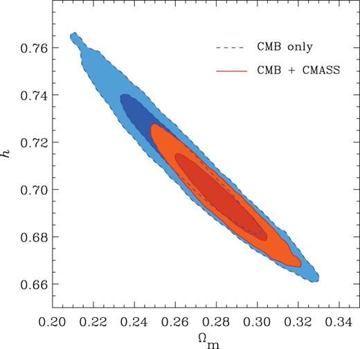
The marginalized constraints in the Ω_m-h plane for the ΛCDM parameter set. The dashed lines show the 68 and 95 per cent contours obtained using CMB information alone. The solid contours correspond to the results obtained from the combination of CMB data plus the shape of the CMASS ξ (s).

Open in new tabDownload slide

The results presented here are completely consistent with those of Anderson et al. (), who explored the cosmological implications of the BAO signal in the CMASS correlation function. From the combination of this information with the latest data from the WMAP satellite, they find Ω_m = 0.298 ± 0.017 and h = 0.684 ± 0.013 when the parameter space is restricted to the ΛCDM model. Although this agreement is not surprising, as the two analyses are based on the same galaxy sample, it is a clear indication of the consistency between the two analysis techniques.

Although consistent within 1σ, the CMASS correlation function prefers somewhat higher values of Ω_m than the CMB data. This difference can be traced back to the values of y_s(z_m) obtained from these data sets individually. In the ΛCDM parameter space, it is possible to obtain a constraint on this quantity on the basis of CMB information alone. In this case, we obtain y_s(z_m) = 0.0762 ± 0.0018, while the CMASS ξ(s) gives y_s(z_m) = 0.0742 ± 0.0014. We will return to this point in Section , where we analyse the clustering properties of the NGC and SGC subsamples separately.

As can be seen in Fig. ⁵, by preferring higher values of Ω_m, the CMASS correlation function also leads to slightly lower values of the Hubble parameter than in the CMB-only case. Although this value is lower than the direct measurement of Riess et al. (), the difference is not statistically significant. As discussed in Anderson et al. () and Mehta et al. (), this difference can be reduced if the effective number of relativistic species, N_eff, is allowed to deviate from the standard value of N_eff = 3.04.

As shown in Table ¹, when the SN and BAO data are added to the analysis, the results point towards values of Ω_m similar to those of the CMB+CMASS case. Combining the information from all these data sets, the recovered values of Ω_m and h are similar to the CMB+CMASS results and the uncertainties are reduced by 33 per cent. In this case, we find and h = 0.6941 ± 0.0081.

Recent analyses have consistently shown evidence of a departure from the scale-invariant primordial power spectrum of scalar fluctuations (Sánchez et al. ; Spergel et al. ; Komatsu et al. , ; Keisler et al. ). Our CMB+CMASS constraint on the spectral index is , increasing the significance of this detection to 4.1σ. This limit is almost unchanged when all data sets are considered, in which case we get . The deviation from scale invariance of the primordial power spectrum has important implications, as most inflationary models predict that the scalar spectral index is less than 1 (Linde ). However, these models also predict the presence of non-zero tensor primordial fluctuations. As we will see in Section , although the constraints on n_s become weaker when the tensor-to-scalar ratio, r, is allowed to vary, we also detect a deviation from scale invariance at the 99.7 per cent confidence level (CL) in this case.

The results from our study show that the standard ΛCDM model is able to accurately describe all the data sets that we have included in our analysis and that the values of its basic parameters are constrained to an accuracy higher than 5 per cent. In the following sections, we focus on constraining possible deviations from this simple model.

5.2 Non-flat models

In this section, we drop the assumption of a flat Universe and allow for models where Ω_k ≠ 0. This parameter space is poorly constrained by the CMB data due to the so-called geometrical degeneracy (Efstathiou & Bond ) relating the physical size of the sound horizon at recombination r_s(z_*), and the angular diameter distance D_A(z_*). The former determines the true physical scale of the acoustic oscillations, while the latter controls its mapping on to angular scales in the sky. Models with the same value of Θ = r_s(z_*)/D_A(z_*) predict the same position of the acoustic peaks in the CMB spectrum and cannot be distinguished on the basis of the primary CMB fluctuations alone. This degeneracy is shown by the dashed lines in Fig. ⁶, which correspond to the 68 and 95 per cent CL contours in the Ω_m–Ω_k plane obtained from the CMB data. The dashed line in panel (a) of Fig. ⁷ shows the corresponding marginalized constraints on Ω_k, which allow for significant deviations from the ΛCDM model value. In this case, we obtain and .

Figure 6

The marginalized posterior distribution in the Ω_m-Ωk plane for the ΛCDM parameter set extended to allow for non-flat models. The dashed lines show the 68 and 95 per cent contours obtained using CMB information alone. The solid contours correspond to the results obtained from the combination of CMB data plus the shape of the CMASS ξ (s). The dotted line corresponds to the ΛCDM model, where Ω_k = 0.

Open in new tabDownload slide

Figure 7

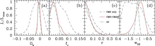
The marginalized, one-dimensional likelihood distribution of the extensions of the ΛCDM model explored in Sections 5.2-5.5. The dashed lines indicate the constraints obtained from CMB information only, solid lines correspond to the results of CMB data plus the shape of the CMASS ξ (s), and the dot-dashed lines show full constraints including also BAO and SN data.

Open in new tabDownload slide

As shown by the solid lines in Fig. ⁶, the constraints on y_s(z_m) and A(z_m) provided by the CMASS correlation function are very effective at breaking this degeneracy, leading to a drastic decrease in the range of allowed values for these parameters. The solid line in panel (a) of Fig. ⁷ corresponds to the posterior distribution of Ω_k obtained from the CMB+CMASS combination, which is in much closer agreement with a flat universe. In this case, we obtain Ω_m = 0.285 ± 0.015 and Ω_k = −0.0043 ± 0.0049.

Anderson et al. () explored the same parameter space using the CMASS BAO signal. From the combination of this measurement with WMAP data, they find Ω_m = 0.299 ± 0.016 and Ω_k = −0.008 ± 0.005. These constraints are in good agreement with findings reported here, although they show a preference for slightly higher values of the matter density parameter.

The inclusion of the SN and BAO data sets does not significantly improve the results over those obtained using the CMB+CMASS combination, with a final constraint of Ω_k = −0.0045 ± 0.0042 obtained from the combination of all data sets. This means that current observations restrict possible variations in the spatial curvature of the Universe up to a level of ΔΩ_k ≃ 4 × 10⁻³.

5.3 Massive neutrinos

In the standard ΛCDM scenario, the dark matter component is given entirely by CDM. However, over the last decade a number of experiments have shown clear evidence of neutrino oscillations, implying that the three known types of neutrino have a non-zero mass and contribute to the total energy budget of the Universe. These observations are sensitive only to the mass-squared differences between neutrino flavours rather than to their absolute masses. Absolute neutrino mass measurements can be obtained from tritium β-decay experiments, which at present provide upper limits of ∑m_ν < 6 eV at the 95 per cent CL (Lobashev ; Eitel ; Lesgourgues & Pastor ). Future experiments like KATRIN are expected to improve these bounds by an order of magnitude (Otten & Weinheimer ). Until then, the best observational window into neutrino masses is provided by cosmological observations, in particular by the combination of CMB and LSS data sets (Hu, Eisenstein & Tegmark ; Elgarøy et al. ; Hannestad ; Sánchez et al. ; Reid et al. ; de Putter et al. ). A variation in the neutrino mass can alter the redshift of matter–radiation equality, thereby affecting the CMB power spectrum. Additionally, until the time when they become non-relativistic, neutrinos free-stream out of density perturbations, suppressing the growth of structures on scales smaller than the horizon at that time, which is a function of their mass. This affects the shape of the matter power spectrum and the correlation function.

In this section, we explore the constraints on the neutrino fraction, f_ν. As current estimates of the differences in the neutrino mass hierarchy are an order of magnitude lower than the constraints on ∑m_ν from cosmological observations, these are not yet sensitive to the masses of individual neutrino eigenvalues; we therefore assume three neutrino species of equal mass. The dashed line in panel (b) of Fig. ⁷ corresponds to the constraints on the neutrino fraction obtained from CMB data alone. In this case, we find f_ν < 0.11 at the 95 per cent CL. The solid line in the same panel shows the effect of including also the information from the shape of the CMASS correlation function, which drastically reduces this limit to f_ν < 0.055 at the 95 per cent CL. Our results can be converted into constraints on the sum of the three neutrino masses using equation to obtain ∑m_ν < 1.4 eV (95 per cent CL) in the CMB-only case, and ∑m_ν < 0.61 eV (95 per cent CL) for CMB data plus the CMASS ξ(s).

Fig. ⁸ shows the 68 and 95 per cent constraints in the Ω_m–f_ν plane. As shown by the dashed lines, when CMB data alone are considered, allowing for f_ν ≠ 0 leads to significantly weaker constraints on Ω_m with respect to the ΛCDM case, with its range of allowed values increasing by more than a factor of 2. The information in the shape of the CMASS correlation function improves these constraints, leading to Ω_m = 0.298 ± 0.019, with a similar accuracy to that of the f_ν = 0 case.

Figure 8

The marginalized posterior distribution in the f ν-Ω_m plane for the ΛCDM parameter set extended by allowing for a non-negligible fraction of massive neutrinos. The dashed lines show the 68 and 95 per cent contours obtained using CMB information alone. The solid contours correspond to the results obtained from the combination of CMB data plus the shape of the CMASS ξ (s).

Open in new tabDownload slide

In a recent analysis, de Putter et al. () explored the constraints on ∑m_ν from the angular power spectrum of a galaxy sample drawn from BOSS DR8 following the CMASS selection criteria, as measured by Ho et al. (). From the combination of this measurement with WMAP7 information, de Putter et al. () obtained a limit of ∑m_ν < 0.56 eV at the 95 per cent CL, which is relaxed to ∑m_ν < 0.90 eV (95 per cent CL) when a more conservative galaxy bias model is implemented. The similarity between these limits and our CMB+CMASS constraint illustrates the power of using the full three-dimensional clustering information, which can compensate for the much larger volume probed by the sample analysed by de Putter et al. ().

Although not directly sensitive to f_ν, the additional information from SN or BAO measurements improves the limits on the neutrino fraction by constraining parameters that are degenerate with this quantity. Combining all data sets we obtain f_ν < 0.049 and ∑m_ν < 0.51 eV at the 95 per cent CL. In the analysis of de Putter et al. (), the inclusion of the SN and H₀ measurements provided a tighter constraint, with ∑m_ν < 0.26 eV at the 95 per cent CL and ∑m_ν < 0.36 eV (95 per cent CL) for the two galaxy bias models they analysed.

An extension of the current analysis to include information from ξ(s) on smaller scales, where it is more sensitive to the effect of neutrino free-streaming, could help to improve the constraints on the neutrino fraction even further. However, as pointed out by Swanson, Percival & Lahav (), effects related to non-linearities and galaxy bias on these scales might impose a limitation on the robustness of clustering measurements as a means to obtain bounds on the neutrino mass. For this reason, the constraints on ∑m_ν presented here should be regarded as conservative, while the full constraining power of the CMASS sample on this quantity will be explored in future studies.

5.4 Tensor modes

We now extend the parameter space of equation to include the tensor-to-scalar amplitude ratio r. This is the parameter space most relevant for the study of inflation as the most simple inflationary models predict non-zero primordial tensor modes (i.e. gravitational waves, Linde ).

Panel (c) of Fig. ⁷ shows the marginalized constraints on r for the cases of CMB data only (dashed lines) and CMB plus the CMASS ξ(s) (solid lines). The constraints imposed on r by CMB information alone are r < 0.21 (95 per cent CL). The CMASS correlation function tightens this limit to r < 0.16 at the 95 per cent CL. This result is only marginally improved by the additional information of the SN and BAO data sets to our final constraint of r < 0.15 (95 per cent CL). These results show good agreement with the constraints of Keisler et al. (), who found r < 0.17 (95 per cent CL) from the combination of the same CMB data sets with BAO and H₀ measurements.

Fig. ⁹ shows the likelihood contours in the n_s–r plane obtained by means of CMB data alone (dashed lines), and its combination with the CMASS ξ(s) (solid lines). Tensor modes contribute to the CMB temperature power spectrum only on large angular scales (ℓ < 400). An increase in the value of r can be compensated for by reducing the amplitude of the scalar modes, thereby maintaining the total amplitude of the temperature fluctuations at a constant level. The consequent decrease of power on smaller angular scales can be compensated for by increasing the scalar spectral index, n_s. Although, as discussed in Keisler et al. (), the information from the small angular scales of the CMB fluctuations provided by SPT does a good job at breaking this degeneracy, a residual relation between these parameters limits the accuracy of their marginalized constraints. By also including the information from the shape of the CMASS correlation function, it is possible to restrict the range of allowed values for these parameters even further. In particular, this combination allows us to detect a deviation from the scale-invariant primordial power spectrum (indicated by the vertical dotted line) with n_s < 1 at the 99.7 per cent CL, even in the presence of tensor modes. This detection has strong implications for the inflationary paradigm.

Figure 9

The marginalized posterior distribution in the n_s-r plane for the ΛCDM parameter set extended by allowing for non-zero primordial tensor modes. The dashed lines show the 68 and 95 per cent contours obtained using CMB information alone. The solid contours correspond to the results obtained from the combination of CMB data plus the shape of the CMASS ξ (s). The dotted line corresponds to the scale-invariant scalar primordial power spectrum, with n_s = 1.

Open in new tabDownload slide

We can explore the implications of our results in terms of constraints on inflationary models by analysing the horizon flow parameters of Schwarz, Terrero-Escalante & García (). These are a hierarchy of parameters describing the evolution of the Hubble factor during inflation. The first parameter is given by ε₁ ≡ −d ln H(N)/dN, where N is the number of e-foldings before the end of inflation at which our pivot scale crosses the Hubble radius during inflation, and the remaining ones are defined through the relation

(22)

The weak energy condition implies that ε₁ > 0, while a necessary condition for inflation is ε₁ < 1 (which implies ). The slow-roll approximation can be expressed as |ε_j| ≪ 1, for all j > 0. In this limit, these parameters satisfy the relations

(23)

(24)

These relations can be used to translate our constraints on n_s and r into the ε₁–ε₂ plane. Fig. ¹⁰ shows the constraints obtained in this way. Marginalizing over ε₂, the combination of CMB data plus the CMASS correlation function implies the limit ε₁ < 0.0097 at the 95 per cent CL. These data sets strongly favour models with positive values of ε₂, in which inflation will end naturally with a violation of the slow-roll approximation (Leach & Liddle ). From the CMB+CMASS combination, we obtain the limit ε₂ > 0 at the 95.8 per cent CL, which is only marginally improved to the 97 per cent CL with the inclusion of the SN and additional BAO measurements.

Figure 10

The marginalized posterior distribution in the ε₁-ε₂ plane for the ΛCDM parameter set extended by allowing for non-zero primordial tensor modes. The dashed lines show the 68 and 95 per cent contours obtained using CMB information alone. The solid contours correspond to the results obtained from the combination of CMB data plus the shape of the CMASS ξ (s). The dot-dashed lines correspond to chaotic inflationary models with p = 1, 2 and 4, as indicated by the labels. The dotted line corresponds to a constant value of N = 60.

Open in new tabDownload slide

The horizon flow parameters are related to the inflaton potential V and its derivatives with respect to the inflaton field ϕ. Then, they can be used to constrain which type of potentials are compatible with the observations (see e.g. Liddle & Leach ; Kinney et al. ; Finelli et al. ). As an example, we explore the constraints on a particular class of models, that of the chaotic (or monomial) inflation, in which the inflationary phase is driven by a potential of the form V(ϕ) ∝ ϕ^p. These models predict a simple relation between the horizon flow parameters, the power-law index, p, and the number of e-foldings, N, given by (Leach & Liddle )

(25)

(26)

The dot–dashed lines in Fig. ¹⁰ correspond to chaotic inflationary models with p = 1, 2 and 4, as indicated by the labels. As can be seen from equations and , a given value of N corresponds approximately to a constant value of ε₂. For the pivot scale considered here, a plausible upper limit for the number of e-foldings is N ≲ 60 (Dodelson & Hui ; Liddle & Leach ), corresponding to ε₂ ≳ 0.017 (indicated by the dotted line in Fig. ¹⁰). If we restrict our analysis to this region of the parameter space, we see that models with p ≳ 2 are strongly disfavoured by the data. In fact, the marginalized distribution for p obtained from the CMB+CMASS combination after applying this prior implies a limit of p < 1.2 at the 95 per cent CL, imposing a strong constraint on the viable chaotic inflationary models.

5.5 The dark energy equation of state

Until now we have assumed that the dark energy component corresponds to a cosmological constant, with a fixed equation of state specified by w_DE = −1. In this section, we allow for more general dark energy models. In Section , we explore the constraints on the value of w_DE (assumed redshift-independent). In Section , we obtain constraints on the time evolution of this parameter, parametrized according to equation . Section deals with the effect of the assumption of a flat universe on the constraints on w_DE.

In these tests, we consider models with w_DE < −1, corresponding to phantom energy (see Copeland, Sami & Tsujikawa , and references therein). When exploring constraints on dynamical dark energy models, these are allowed to cross the so-called phantom divide, w_DE = −1. In the framework of general relativity, a single fluid, or a single scalar field without higher derivatives, cannot cross this threshold since it would become gravitationally unstable (Feng, Wang & Xiulian ; Hu ; Vikman ; Xia et al. ), requiring at least one extra degree of freedom. However, models with more degrees of freedom are difficult to implement in general dark energy studies. Here we follow the parametrized post-Friedmann approach of Fang et al. (), as implemented in camb, which provides a simple solution to these problems for models in which the dark energy component is smooth compared to the dark matter. Alternatively, as proposed by Zhao et al. (), it is possible to consider the dark energy perturbations using a two-field model, with one of the fields being quintessence like and the other one phantom like (e.g. the quintom model proposed in Feng et al. ) without introducing new internal degrees of freedom. Both approaches give consistent results.

2010 Time-independent dark energy equation of state

In this section, we explore the constraints on the parameter set of equation extended by including the redshift-independent value of w_DE as an additional parameter. The dashed lines in Fig. ¹¹ show the two-dimensional marginalized constraints in the Ω_m–w_DE plane obtained from CMB data alone. There is a strong degeneracy between these parameters along which different models predict the same angular position for the peaks in the CMB power spectrum. This is analogous to the geometrical degeneracy described in Section , corresponding to models with constant values of Θ. This degeneracy leads to poor one-dimensional constraints of and .

Figure 11

The marginalized posterior distribution in the Ω_m-ω_DE plane for the ΛCDM parameter set extended by including the redshift-independent value of ωDE as an additional parameter. The dashed lines show the 68 and 95 per cent contours obtained using CMB information alone. The solid contours correspond to the results obtained from the combination of CMB data plus the shape of the CMASS ξ (s). The dot-dashed lines indicate the results obtained from the full data set combination (CMB+CMASS+SN+BAO). The dotted line corresponds to the ΛCDM model, where ω_DE =-1.

Open in new tabDownload slide

The solid lines in Fig. ¹¹ show the effect of including the CMASS correlation function in the analysis. The constant-Θ degeneracy can be partially broken by providing an additional distance constraint. The constraint on y_s(z_m) provided by ξ(s) breaks the degeneracy between Ω_m and w_DE, tightening the constraints on the dark energy equation of state. The impact of including the CMASS correlation function on the marginalized constraints on w_DE can be seen in panel (d) of Fig. ⁷ where the dashed lines correspond to the result of the CMB-only case and the solid lines to the result of the CMB+CMASS combination. In this case, we obtain and , in good agreement with a cosmological constant.

From the combination of the BAO signal inferred from the CMASS P(k) and ξ(s) with WMAP data, Anderson et al. () obtained the constraints Ω_m = 0.323 ± 0.043 and w_DE = −0.87 ± 0.24, in good agreement with our findings. As in the previous parameter spaces, this is a clear indication of the consistency between the two analysis techniques. The extra information in the shape of ξ(s) improves the constraints on the dark energy equation of state by ∼20 per cent with respect to the BAO-only result, indicating that, at this redshift, most of the information on this parameter is obtained through the measurement of y_s.

In a recent analysis, Montesano et al. () used the full shape of the power spectrum of a sample of LRGs from the final SDSS-II, combined with a compilation of CMB experiments, to obtain the constraint w_DE = −1.02 ± 0.13. Mehta et al. () combined the BAO distance measurement derived by Padmanabhan et al. () and Xu et al. () from the same galaxy sample with WMAP data, to obtain w_DE = −0.92 ± 0.13. As these measurements are based on observations at lower redshifts, which are more sensitive to variations in w_DE, they provide slightly tighter constraints on this parameter than the CMB+CMASS combination.

Including also the additional BAO data in the analysis gives similar results to the CMB+CMASS case, with a constraint on the dark energy equation of state of . When the SN data are considered in the analysis instead of the BAO data, the resulting constraints are in better agreement with the standard ΛCDM value, with . It is interesting to note that this result is mostly driven by the CMASS+SN combination. In fact, the combined information from these two data sets provides the constraint w_DE = −1.04 ± 0.11, independently of any CMB data. Our final constraints obtained from the combination of all data sets are shown by the dot–dashed lines in Fig. ¹¹, corresponding to Ω_m = 0.281 ± 0.012 and . This result is in excellent agreement with the standard ΛCDM model value of w_DE = −1, indicated by a dotted line in Fig. ¹¹.

The time evolution of w_DE

In the ΛCDM model, the equation-of-state parameter is characterized by the fixed value w_DE = −1 at all times. A detection of a deviation from this prediction would be a clear signature of the need of alternative dark energy models. In this section, we explore the constraints on the redshift dependence of w_DE which we parametrize according to equation .

The dashed lines in Fig. ¹² show the two-dimensional marginalized constraints in the w₀–w_a plane obtained from the CMB data alone. This case provides only weak constraints on these parameters, allowing for models where the value of w_DE can vary significantly over time. The inclusion of the CMASS correlation function reduces this allowed region to a linear degeneracy between w₀ and w_a which can still accommodate large deviations from the ΛCDM values, indicated by the dotted lines. At least a third data set is required to obtain more restrictive constraints. In the CMB+CMASS+SN case, we obtain w₀ = −1.09 ± 0.11 and , which change to w₀ = −0.95 ± 0.27 and if the SN data are replaced by the additional BAO measurements. The dot–dashed lines in Fig. ¹² correspond to our tightest constraints, obtained by combining all data sets, where we obtain the marginalized values w₀ = −1.08 ± 0.11 and w_a = 0.23 ± 0.42.

Figure 12

The marginalized posterior distribution in the ω₀-ω_a plane for the ΛCDM parameter set extended by allowing for variations on ω_DE(a), parametrized as in equation (12). The dashed lines show the 68 and 95 per cent contours obtained using CMB information alone. The solid contours correspond to the results obtained from the combination of CMB data plus the shape of the CMASS ξ (s). The dot-dashed lines indicate the results obtained from the full data set combination (CMB+CMASS+SN+BAO). The dotted lines correspond to the canonical values in the ΛCDM model.

Open in new tabDownload slide

A useful quantity to characterize the constraints on the redshift evolution of the dark energy equation of state is the pivot redshift, z_p, defined as the point where the uncertainty on w_DE(a) is minimized (Huterer & Turner ; Hu & Jain ; Albrecht et al. ). The parametrization of equation implies that this redshift corresponds to the scalefactor

(27)

The corresponding pivot redshift for the CMB+CMASS combination is given by z_p = 1.21, for which we obtain w_DE(z_p = 1.21) = −0.94 ± 0.20. The pivot redshift for the combination of all data sets is z_p = 0.23, which corresponds to our tightest constraint on the dark energy equation of state, with w_DE(z_p = 0.23) = −1.040 ± 0.072, in good agreement with a cosmological constant.

Dark energy and curvature

We now explore the constraints on the dark energy equation of state (assumed time-independent) when the assumption of a flat Universe is dropped. This parameter space presents similar characteristics to the one studied in Section , where the dark energy equation of state is allowed to evolve over time. As discussed by Komatsu et al. () and Sánchez et al. (), when both w_DE and Ω_k are allowed to vary, the one-dimensional degeneracies corresponding to constant values of Θ obtained from the CMB observations in the analyses of Sections and gain an extra degree of freedom. As shown by the dashed lines in Fig. ¹³, when projected in the w_DE–Ω_k plane, this two-dimensional degeneracy extends over a large region of the parameter space. The solid lines in Fig. ¹³ show the resulting constraints from the CMB+CMASS combination. Although the constraint on y_s(z_m) provided by the CMASS correlation function substantially reduces the allowed region for these parameters, the remaining degeneracy between them corresponds to poor one-dimensional marginalized restrictions.

Figure 13

The marginalized posterior distribution in the ω_DE-ωk plane for the ΛCDM parameter set extended by allowing for simultaneous variations on ω_DE (assumed time-independent) and Ω_k. The dashed lines show the 68 and 95 per cent contours obtained using CMB information alone. The solid contours correspond to the results obtained from the combination of CMB data plus the shape of the CMASS ξ (s). The dot-dashed lines indicate the results obtained from the full data set combination (CMB+CMASS+SN+BAO). The dotted lines correspond to the values of these parameters in the ΛCDM model.

Open in new tabDownload slide

The distance measurements provided by the additional BAO or SN data sets can break the remaining degeneracy, leading to meaningful constraints on these parameters. The dot–dashed lines in Fig. ¹³ correspond to the constraints obtained with the combination of all four data sets, showing good agreement with the ΛCDM model values (indicated by the dotted lines). In this case, we obtain Ω_k = −0.0054 ± 0.0044 and w_DE = −1.060 ± 0.075, with similar accuracies to the constraints obtained when each of these parameters is varied independently (Sections and ).

6 THE CLUSTERING SIGNAL IN THE NORTHERN AND SOUTHERN GALACTIC HEMISPHERES

Our analysis is based on the full CMASS sample, combining the NGC and SGC data. Compared to the NGC observations, the SGC observations correspond to a region with larger average Galactic extinction and were taken under higher airmass and sky background and over different periods of time. These differences make the NGC–SGC split a sensible cut to study the clustering properties of these subsamples individually. In fact, when analysed separately, the clustering of the NGC and SGC CMASS subsamples presents some intriguing differences. This can be seen in Fig. ¹⁴, which shows the measurements of ξ(s) in these two regions, obtained as described in Section . It is clear that, although they exhibit the same overall shape, the BAO feature in the SGC subsample has a higher amplitude, and its centroid is located at smaller scales than in the NGC subsample. In this section, we explore the significance of these differences and their implications on the obtained cosmological constraints.

Figure 14

Large-scale correlation function of the NGC (circles) and SGC (squares) CMASS subsamples. The dashed line corresponds to the bestfitting ΛCDM model obtained by combining the CMB data with the information from the shape of the NGC correlation function. Although the two measurements exhibit the same broad-band shape, in the SGC data the BAO peak has a larger amplitude and is located at smaller scales than in the NGC ξ (s).

Open in new tabDownload slide

Ross et al. () performed a comprehensive analysis of the differences between the NGC and SGC CMASS subsamples and found no treatment of the data that could alleviate them. Schlafly et al. () and Schlafly & Finkbeiner () found small systematic offsets between the colours of SDSS objects in the NGC and SGC subsamples, which lead to slightly different selection criteria for the CMASS sample in the two Galactic hemispheres. Ross et al. () found a 3.2 per cent difference in the number density of CMASS targets between the NGC and SGC subsamples, which reduces to 0.3 per cent when the offset of Schlafly & Finkbeiner () is applied to the galaxies in the SGC subsample before applying the CMASS selection criteria. However, Ross et al. () found that these factors do not produce a measurable effect on the clustering signal of the SGC CMASS sample, and the differences between the correlation functions of the SGC and NGC subsamples remain the same.

The consistency between the measurements in the NGC and SGC subsamples can be assessed by examining the difference ξ_NGC(s) − ξ_SGC(s). As these regions correspond to well-separated volumes, we can neglect the covariance between them and estimate the covariance matrix for this difference simply as , where and correspond to the covariance matrices of the individual NGC and SGC regions, respectively. The consistency of the difference ξ_NGC(s) − ξ_SGC(s) with cosmic variance can be estimated from its χ² value, with respect to . In the range of scales used in our analysis, 40 < s/(h⁻¹ Mpc) < 200, we find χ² = 53.9 for 41 data points. This number changes to χ² = 25.2 for 15 points if the test is restricted to the range of scales of the BAO peak [70 < s/(h⁻¹ Mpc) < 130]. Using a different bin size of Δs = 7 h⁻¹ Mpc, Ross et al. () performed the same test and found similar values of χ² per degree of freedom. This result shows quantitatively that the general shapes of these measurements are in agreement, and the differences between them are localized at the scales of the acoustic peak. Note, however, that this is the range of scales from where the constraints on y_s are obtained.

Another view of this is presented in Fig. ¹⁵, which shows the two-dimensional marginalized constraints in the A(z_m)–y_s(z_m) plane. While the two measurements point towards consistent values of A(z_m), with A(z_m) = 0.426 ± 0.021 and 0.447 ± 0.030 from the NGC and SGC subsamples, respectively, the different locations of the acoustic peak inferred from these regions lead to y_s(z_m) = 0.0762 ± 0.0015 and 0.0704 ± 0.0017, respectively, which are approximately 2σ apart. Despite the fact that the errors in the SCG correlation function are almost a factor of 2 larger than those of its NGC counterpart, the accuracies of the constraints on y_s obtained from these measurements are similar. This is due to the high amplitude of the BAO bump in the SGC ξ(s) which, as shown in Fig. ¹⁴, gives a precise determination of the centroid of the peak, leading to a slightly smaller than expected uncertainty on y_s. As was pointed out in Section , within the ΛCDM parameter space the CMB data alone are sufficient to obtain the estimate y_s(z_m) = 0.0762 ± 0.0018. This value shows a remarkable consistency with the result obtained from the NGC subsample. A comparison between Fig. ² and ¹⁴ shows that, although the correlation function of the full CMASS sample is dominated by that of the NGC subsample, which covers a larger volume, adding the data from the SGC subsample moves the BAO peak towards somewhat smaller scales, leading to the result y_s(z_m) = 0.0742 ± 0.0014.

Figure 15

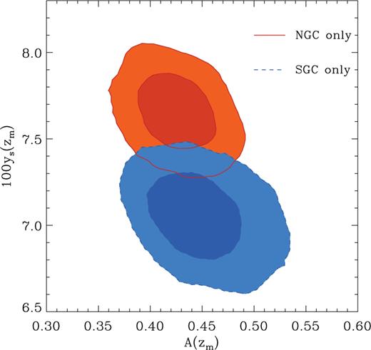
The marginalized posterior distribution in the A(z_m)-y_s(z_m) plane obtained from the correlation function of the NGC (solid lines) and SGC (dashed lines) CMASS subsamples. The contours correspond to the 68 and 95 per cent CL. While the two measurements point towards consistent values of A(z_m), their preferred values of y_s(z_m) deviate by approximately 2σ.

Open in new tabDownload slide

The conclusion from the tests of Ross et al. () is that the differences between the NGC and SGC subsamples are simply due to a statistical fluctuation. However, as the data in the NGC subsample cover a volume 3.7 times larger, providing a better knowledge of the survey selection function, for completeness we also discuss here the constraints on the parameter spaces of Section obtained from the combination of the correlation function of the NGC subsample with our CMB data set. We do not consider here, however, the extension of the ΛCDM parameter space in which both w_DE and Ω_k are allowed to float since, as discussed in Section , the combination of CMB data with a measurement of ξ(s) is not enough to break the strong degeneracy between these parameters. The complete list of parameter constraints obtained from the CMB+NGC combination is summarized in Table ⁸.

For the ΛCDM parameter space, the mean values for the cosmological parameters obtained in the CMB+NGC case are in closer agreement with those obtained by means of the CMB data alone than in the full CMB+CMASS case. For example, in the CMB+NGC case we find the constraints of Ω_m = 0.265 ± 0.014 and h = 0.711 ± 0.012, in excellent agreement with the CMB-only results of Ω_m = 0.266 ± 0.024 and h = 0.710 ± 0.20. The slightly higher value of the Hubble parameter obtained in this case reduces the difference with the measurement of Riess et al. () to the 1σ level.

When the curvature of the Universe is included as a free parameter, the value of y_s(z_m) from the NGC subsample breaks the geometrical degeneracy in the CMB data closer to the locus of the flat models, yielding a constraint of Ω_k = −0.0002 ± 0.0049, completely consistent with the flat Universe prediction from the inflationary paradigm.

When constraining the fraction of massive neutrinos, the CMB+NGC combination yields f_ν < 0.044 and ∑m_ν < 0.52 eV at the 95 per cent CL. These limits are slightly tighter than those obtained in the CMB+CMASS case. Regarding the constraints on the tensor-to-scalar ratio, from the CMB+NGC combination we find r < 0.17 at the 95 per cent CL, which is equivalent to the limit found using the full CMASS ξ(s), albeit with a preference for lower matter density values, with Ω_m = 0.276 ± 0.016

The results for the dark energy related parameter spaces also change when the full CMASS ξ(s) is replaced by the one of the NGC subsample. In this case, we obtain weaker constraints, with and w_DE = −1.14 ± 0.26. When equation is used to explore the redshift dependence of the dark energy equation of state, we find and and a constraint of w_DE(z_p) = −1.21 ± 0.26 at the pivot redshift of z_p = 0.96.

In all cases analysed, when we restrict our analysis to the NGC CMASS subsample the constraints change at most by 1σ. This is in agreement with the results of Ross et al. (), who found the same level of consistency. In general, we find that the NGC data point towards slightly lower values of Ω_m and higher ones of h than those obtained from the full CMASS sample and in closer agreement with the CMB-only case. It should be emphasized, however, that the extensive tests of Ross et al. (), together with our internal investigations, show no reason for preferring the measurements from the NGC subsample alone to the measurements from the full CMASS sample, which provides our best picture of the clustering of galaxies at z ≃ 0.57.

7 Conclusions

We have presented an analysis of the cosmological implications of the monopole of the redshift-space two-point correlation function, ξ(s), measured from the BOSS DR9 CMASS sample. The large volume and average number density of this sample make it ideally suited for LSS analysis. The information contained in the full shape of the CMASS ξ(s) allowed us to obtain accurate constraints of the parameters y_s(z_m) and A(z_m), given by equations and , respectively. By adopting an explicit, perturbation theory based model for the correlation function in the mildly non-linear regime, and marginalizing over its uncertain parameters, we are able to exploit information beyond that in the scale of the BAO peak alone. We combined this information with that of additional cosmological probes, including CMB, SN and BAO measurements from other data sets, to derive constraints on cosmological parameters. We studied the parameters of the ΛCDM parameter space, and a number of its extensions. The main results from our analysis can be summarized as follows:

• Our results show that the simple ΛCDM model is able to describe all the data sets that we have included in our analysis. Given the different nature of these observations and the range of redshifts they probe, this is not a minor achievement. The basic parameters of this model are constrained to an accuracy better than 5 per cent, a clear demonstration of the constraining power of observations in the current era of precision cosmology.

• Fig. ⁷ summarizes our constraints on possible extensions of the standard ΛCDM model. We considered non-flat models, massive neutrinos, non-zero primordial tensor fluctuations, and more general dark energy models. In all of these cases, the inclusion of the CMASS ξ(s) in the analysis significantly improves the obtained constraints with respect to those obtained using the CMB data alone. Our results show no significant evidence of deviations from the ΛCDM picture, which can still be considered as our best cosmological model.

• The information provided by the CMASS correlation function is essential to obtain tight constraints on the curvature of the Universe. We obtain the constraint from the CMB+CMASS combination which is not significantly improved by adding information from SN or other BAO data.

• When massive neutrinos are considered in the analysis, we find a constraint of f_ν < 0.056 at the 95 per cent CL, implying a limit of ∑m_ν < 0.61 eV on the sum of the three neutrino species. This limit is improved to ∑m_ν < 0.51 eV when the SN and BAO data are added to the analysis.

• When considering tensor modes, the CMB+CMASS combination allowed us to obtain a limit on the tensor-to-scalar amplitude ratio of r < 0.16 at the 95 per cent CL, which is almost unchanged by considering additional data sets. The combination of CMB data with the shape of the CMASS correlation function reveals a clear signature of deviation from scale invariance, with n_s < 1 at the 99.7 per cent CL, also in the presence of tensor modes.

• We explored models where the dark energy component does not correspond to a cosmological constant and found no signature of deviation from the standard ΛCDM model. When the value of w_DE, assumed time-independent, is allowed to vary, the CMB+CMASS combination provides the constraint . Interestingly, the CMASS+SN combination alone provides a tighter constraint, with w_DE = −1.04 ± 0.11, independently of any CMB data. Our tighter constraints are obtained from the combination of all data sets, with , in good agreement with a cosmological constant. This result does not change significantly if the assumption of a flat universe is relaxed. We also find no evidence of redshift evolution of w_DE.

• Our results are in excellent agreement with those of Anderson et al. () and Reid et al. (), who explored the cosmological implications of the BAO and redshift-space distortion measurements in the CMASS sample. This highlights the consistency between the different analysis techniques implemented in each of these studies, and provides a reassuring demonstration of the robustness of our results.

• We studied the clustering of the NGC and SGC regions separately. The overall shapes of the correlation functions in these two subsamples show good agreement, but they differ in the location and amplitude of BAO peak. This translates into constraints of y_s(z_m) which differ at the 2σ level. Ross et al. () performed a detailed analysis of the clustering signal in these regions and found no evidence of additional systematic effects in the SGC data, indicating that the observed differences are simply due to a statistical fluctuation. For completeness, we explored the constraints obtained when the NGC correlation function is used in combination with our CMB data sets. In all cases, our results remain unchanged within 1σ, with the NGC data pointing towards slightly lower values of Ω_m and higher ones of h than those obtained from the full CMASS sample.

The current analysis is based on the first spectroscopic data release of BOSS. The larger volume that will be probed by subsequent data releases, plus the extension of the analysis to the lower redshift BOSS galaxies, will reduce the uncertainties in the measurement of ξ(s) and the calibration of the corrections for potential systematic effects, providing even more accurate views of the LSS clustering pattern in the Universe. This improvement will be accompanied by the release of the CMB power spectrum measurements from the Planck satellite in early 2013. The combination of these data sets will undoubtedly provide new, more stringent constraints on cosmological parameters, and will open up the possibility to explore additional extensions to the ΛCDM model which have not yet been fully explored.

Acknowledgments

We would like to thank Ryan Keisler for his help with the implementation of the SPT likelihood code in CosmoMC. We also thank Bradford Benson for helping us find a bug in our modifications to CosmoMC by pointing out a discrepancy between our constraints on the equation of state of dark energy using only CMB data and the reported values by the WMAP team. AGS would like to thank all users of the Pan-STARRS cluster in Garching for their patience and support. CGS and JAR acknowledge funding from project AYA2010-21766-C03-02 of the Spanish Ministry of Science and Innovation (MICINN). AJR is grateful to the UK Science and Technology Facilities Council for financial support through the grant ST/I001204/1. WP is grateful for support from the UK Science and Technology Facilities Research Council, the Leverhulme Trust and the European Research Council. FP acknowledges support from the Spanish MICINNs Consolider grant MultiDark CSD2009-00064. JAR is a Ramón y Cajal fellow of the Spanish Ministry of Science and Innovation (MICINN).

Funding for SDSS-III has been provided by the Alfred P. Sloan Foundation, the Participating Institutions, the National Science Foundation, and the US Department of Energy.

SDSS-III is managed by the Astrophysical Research Consortium for the Participating Institutions of the SDSS-III Collaboration including the University of Arizona, the Brazilian Participation Group, Brookhaven National Laboratory, University of Cambridge, Carnegie Mellon University, University of Florida, the French Participation Group, the German Participation Group, Harvard University, the Instituto de Astrofisica de Canarias, the Michigan State/Notre Dame/JINA Participation Group, The Johns Hopkins University, Lawrence Berkeley National Laboratory, Max Planck Institute for Astrophysics, Max Planck Institute for Extraterrestrial Physics, New Mexico State University, New York University, The Ohio State University, The Pennsylvania State University, University of Portsmouth, Princeton University, the Spanish Participation Group, University of Tokyo, University of Utah, Vanderbilt University, University of Virginia, University of Washington and Yale University.

We acknowledge the use of the Legacy Archive for Microwave Background Data Analysis (LAMBDA). Support for LAMBDA is provided by the NASA Office of Space Science.

References

A Appendix

Summary of the Obtained Cosmological Constraints

In this section, we summarize the constraints on cosmological parameters obtained using different combinations of the data sets described in Sections and . Table ¹ lists the 68 per cent confidence limits on the parameters of the ΛCDM model, as discussed in Section . Tables correspond to the extensions of this parameter space analysed in Sections –. Finally, Table ⁸ presents the constraints on these parameter spaces, obtained from the combination of the correlation function of the NGC subsample with the CMB data.

Table 1

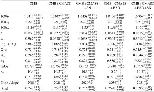
The marginalized 68 per cent constraints on the cosmological parameters of the ΛCDM model obtained using different combinations of the data sets described in Sections 2.1 and 3.

Open in new tabDownload slide

Table 2

The marginalized 68 per cent allowed regions on the cosmological parameters of the ΛCDM model extended by adding Ωk as a free parameter, obtained using different combinations of the data sets described in Sections 2.1 and 3.

Open in new tabDownload slide

Table 3

The marginalized 68 per cent allowed regions on the cosmological parameters of the ΛCDM model extended by adding f ν as a free parameter, obtained using different combinations of the data sets described in Sections 2.1 and 3.

Open in new tabDownload slide

Table 4

The marginalized 68 per cent allowed regions on the cosmological parameters of the ΛCDM model extended by allowing for non-zero primordial tensor modes, obtained using different combinations of the data sets described in Sections 2.1 and 3.

Open in new tabDownload slide

Table 5

The marginalized 68 per cent allowed regions on the cosmological parameters of the ΛCDM model extended by including the redshift-independent value of ω_DE as an additional parameter, obtained using different combinations of the data sets described in Sections 2.1 and 3.

Open in new tabDownload slide

Table 6

The marginalized 68 per cent allowed regions on the cosmological parameters of the ΛsCDM model extended by allowing for variations on ω_DE(a) (parametrized according to equation 12), obtained using different combinations of the data sets described in Sections 2.1 and 3.

Open in new tabDownload slide

Table 7

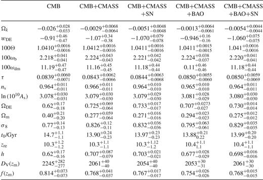
The marginalized 68 per cent allowed regions on the cosmological parameters of the ΛCDM model extended by allowing for simultaneous variations on ω_DE (assumed time-independent) and Ω_k, obtained using different combinations of the data sets described in Sections 2.1 and 3.

Open in new tabDownload slide

Table 8

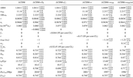
The marginalized per cent allowed regions on the cosmological parameters of the ΛCDM model and its extensions, obtained by combining the CMB data with the correlation function of the NGC CMASS subsample

Open in new tabDownload slide

Author notes