OGLE-2008-BLG-510: first automated real-time detection of a weak microlensing anomaly - brown dwarf or stellar binary?^⋆ Free

Abstract

1 Introduction

The ‘most curious’ effect of gravitational microlensing (Einstein 1936; Paczyński 1986) lets us extend our knowledge of planetary systems (Mao & Paczyński 1991) to a region of parameter space unreachable by other methods and thus populated with intriguing surprises. Microlensing has already impressively demonstrated its sensitivity to super-Earths with the detection of a 5 M_⊕ (uncertain to a factor of 2) planet (Beaulieu et al. 2006), and it reaches down even to about the mass of the Moon (Paczyński 1996).

The transient nature of microlensing events means that rather than the characterization of individual systems, it is the population statistics that will provide the major scientific return of observational campaigns. Meaningful statistics will however only arise with a controlled experiment, following well-defined fully deterministic and reproducible procedures. In fact, the observed sample is a statistical representation of the true population under the respective detection efficiency of the experiment. An analysis of 13 events with peak magnifications A₀ ≥ 200 observed between 2005 and 2008 provided the first well-defined sample (Gould et al. 2010). In contrast, the various claims of planetary signatures and further potential signatures come with vastly different degrees of evidence and arise from different data treatments and applied criteria (Dominik 2010) as well as observing campaigns following different strategies.

While the selection of highly magnified peaks is relatively easily controllable, and these come with a particularly large sensitivity to planetary companions to the lens star (Griest & Safizadeh 1998; Horne, Snodgrass & Tsapras 2009), their rarity poses a fundamental limit to planet abundance measurements. Moreover, the finite size of the source stars strongly disfavours the immediate peak region for planet masses ≲ 10 M_⊕, where a large magnification results from source and lens star being very closely aligned. In contrast, during the wing phases of a microlensing event, planets are more easily recognized with larger sources because of an increased signal duration, as long as the amplitude exceeds the threshold given by the photometric accuracy (cf. Han 2007). It is therefore not a surprise at all that the two least massive planets found so far with unambiguous evidence from a well-covered anomaly, namely OGLE-2005-BLG-390Lb (Beaulieu et al. 2006) and MOA-2009-BLG-266Lb (Muraki et al. 2011), come with an off-peak signature at moderate magnification with a larger source star.

An event duration of about a month and a probability of ∼10⁻⁶ for an observed Galactic bulge star to be substantially brightened at any given time (Paczyński 1991; Kiraga & Paczyński 1994) called for a two-step strategy of survey and follow-up observations (Gould & Loeb 1992). In such a scheme, surveys monitor ≲ 10⁸ stars on a daily basis for ongoing microlensing events (Udalski et al. 1992; Alcock et al. 1997; Bond et al. 2001; Afonso et al. 2003), whereas roughly hourly sampling of the most promising ongoing events with a network of telescopes supporting round-the-clock coverage and photometric accuracy of ≲ 2 per cent allows not only the detection of planetary signatures, but also their characterization (Albrow et al. 1998; Dominik et al. 2002; Burgdorf et al. 2007). While real-time alert systems on ongoing anomalies (Udalski et al. 1994; Alcock et al. 1996), combined with the real-time provision of photometric data, paved the way for efficient target selection by follow-up campaigns, the real-time identification of planetary signatures and other deviations from ordinary light curves so-called anomalies (Udalski 2003; Dominik et al. 2007) allowed a transition to a three-step-approach, where the regular follow-up cadence can be relaxed in favour of monitoring more events, and a further step of anomaly monitoring at ∼5–10 min cadence (including target-of-opportunity observations) is added, suitable to extend the exploration to planets of Earth mass and below.

The recent and upcoming increase of the field-of-view of microlensing surveys (MOA: 2.2 deg², OGLE-IV: 1.4 deg², Wise Observatory: 1 deg², KMTNet: 4 deg²) allows for sampling intervals as small as 10–15 min. This almost merges the different stages with regard to cadence, but the surveys are to choose the exposure time (determining the photometric accuracy) per field rather than per target star. Moreover, they cannot compete with the angular resolution possible with lucky-imaging cameras (Fried 1978; Tubbs et al. 2002; Jørgensen 2008; Grundahl et al. 2009), given that this technique is incompatible with a wide field-of-view. This leaves a most relevant role for ground-based follow-up networks in breaking into the regime below Earth mass, in particular with space-based surveys (Bennett & Rhie 2002) at least about a decade away.

It is rather straightforward to run microlensing surveys in a fully deterministic way, but it is very challenging to achieve the same for both the target selection process of follow-up campaigns and the real-time anomaly identification. The pioneering use of robotic telescopes in this field with the RoboNet campaigns (Burgdorf et al. 2007; Tsapras et al. 2009) led Horne et al. (2009) to devise the first workable target prioritization algorithm. The Optical Gravitational Lensing Experiment (OGLE) EEWS (Udalski 2003) was the first automated system to detect potential deviations from ordinary microlensing light curves, which flagged such suspicions to humans who would then take a decision. In contrast, the signalmen anomaly detector (Dominik et al. 2007) was designed just to rely on statistics and request further data from telescopes until a decision for or against an ongoing anomaly can be taken with sufficient confidence. signalmen has already demonstrated its power by detecting the first sign of finite-source effects in MOA-2007-BLG-233/OGLE-2007-BLG-302 (Choi et al. 2012) – ahead of any humans – and leading to the first alerts sent to observing teams that resulted in crucial data being taken on OGLE-2007-BLG-355/MOA-2007-BLG-278 (Han et al. 2009) and OGLE-2007-BLG-368/MOA-2007-BLG-308 (Sumi et al. 2010), the latter involving a planet of ∼20 M_⊕. signalmen is now fully embedded into the Automated Robotic Terrestrial Exoplanet Microlensing Search (ARTEMiS) software system (Dominik et al. 2008a,b) for data modelling and visualization, anomaly detection and target selection. The 2008 Microlensing Network for the Detection of Small Terrestrial Exoplanets (MiNDSTEp) campaign directed by ARTEMiS provided a proof of concept for fully deterministic follow-up observations (Dominik et al. 2010).

In event OGLE-2008-BLG-510, discussed in detail here, evidence for an ongoing microlensing anomaly was for the first time obtained by an automated feedback loop realized with the ARTEMiS system, without any human intervention. This demonstrates that robotic or quasi-robotic follow-up campaigns can operate efficiently.

A fundamental difficulty in obtaining planet population statistics arises from the fact that many microlensing events show weak or ambiguous anomalies, sometimes with poor quality data, which are left aside because the time investment in their modelling would be too high compared to the dubious perspective to draw any definite conclusions. Indeed such events represent a silver mine for statistical studies yet to be designed. Event OGLE-2002-BLG-55 has already been very rightfully classified as ‘a possible planetary event’ (Jaroszyński & Paczyński 2002; Gaudi & Han 2004), where ambiguities are mainly the result of sparse data over the suspected anomaly. Here, we show that OGLE-2008-BLG-510 makes another example for ambiguities, which in this case arise due to the lack of prominent features of the weak perturbation near the peak of the microlensing event. Given that χ² is not a powerful discriminator, in particular, in the absence of proper noise models (e.g. Ansari 1994), it needs a careful analysis of the constraints on parameter space posed by the data rather than just a claim of a ‘most favourable’ model. In fact, the latter might point to excitingly exotic configurations, but it must not be forgotten that maximum-likelihood estimates (equalling to χ² minimization under the assumption of measurement uncertainties being normally distributed) are not guaranteed to be anywhere near the true value. We therefore apply a modelling approach that is based on a full classification of the finite number of morphologies of microlensing light curves in order to make sure that no feature of the intricate parameter space is missed (Bozza et al. in preparation).

Dominik (1998b) argued that the apparent paucity of microlensing events reported that involve source rather than lens binaries (e.g. Griest & Hu 1992) could be the result of an intrinsic lack of characteristic features, but despite a further analysis by Han & Jeong (1998), the puzzle is not solved yet. Moreover, while all estimates of the planet abundance from microlensing observations indicate a quite moderate number of massive gas giants (Gould et al. 2010; Sumi et al. 2010; Dominik 2011; Cassan et al. 2012), the small number of reported brown dwarfs (cf. Dominik 2010), much easier to detect, seems even more striking. As we will see, the case of OGLE-2008-BLG-510 appears to be linked to both. Maybe the full exploration of parameter space for events with weak or without any obvious anomaly features will get us closer to understanding this issue which is of primary relevance for deriving abundance statistics.

In Section 2, we report the observations of OGLE-2008-BLG-510 along with the record of the anomaly detection process and the strategic choices made. Section 3 discusses the data reduction and the limitations arising from apparent systematics, Section 4 details the modelling process, whereas the competing physical scenarios are discussed in Section 5, before we present final conclusions in Section 6.

2 Observations and Anomaly Detection

The microlensing event OGLE-2008-BLG-510 at RA 18^h09^m37^s.65 and Dec. −26°02′26″.70 (J2000), first discovered by the OGLE team, was subsequently monitored by several campaigns with telescopes at various longitudes (see Table 1) and independently detected as MOA-2008-BLG-369 by the Microlensing Observations in Astrophysics (MOA) team. Table 2 presents a timeline of observations and anomaly detection.

Table 1

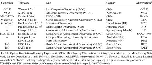
Overview of campaigns that monitored OGLE--BLG-510 and the telescopes used.

Open in new tabDownload slide

Table 2

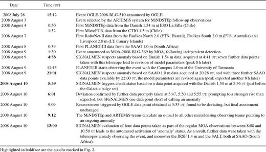
Timeline of OGLE--BLG-510 observations and anomaly detection.

Open in new tabDownload slide

When the follow-up observations started (2008 August 4), the event magnification was estimated by signalmen (Dominik et al. 2007) to be A∼ 3.9, which for a baseline magnitude I∼ 19.23 and absence of blending means an observed target magnitude I∼ 17.75. The event magnification implied an initial sampling interval for the MiNDSTEp campaign of τ = 60 min according to the MiNDSTEp strategy (Dominik et al. 2010).

The OGLE, MOA, MiNDSTEp, RoboNet-II and Probing Lensing Anomalies NETwork (PLANET)-III groups all had real-time data reduction pipelines running, and with efficient data transfer, photometric measurements were available for assessment of anomalous behaviour by signalmen shortly after the observations had taken place. While the MicroFUN team also took care of timely provision of their data, we could not manage at that time to get a data link with signalmen installed, but since 2009 we have been enjoying an efficient rsync connection.¹ RoboNet data processing unfortunately had to cease due to fire in Santa Barbara in early July. After resuming operations and working through the backlog, RoboNet data on OGLE-2008-BLG-510 were not available before 2008 August 23.

The signalmen anomaly detector (Dominik et al. 2007) is based on the principle that real-time photometry and flexible scheduling allow requesting further data for assessment until a decision about an ongoing anomaly can be taken with sufficient confidence. The specific choice of the adopted algorithm comes with substantial arbitrariness, where the power for detecting anomalies needs to be balanced carefully against the false alert rate. signalmen assigns a ‘status’ to each of the events, which is either ‘ordinary’ (= there is no ongoing anomaly), ‘anomaly’ (= there is an ongoing anomaly), or ‘check’ (= there may or may not be an ongoing anomaly). This ‘status’ triggers a respective response: ‘ordinary’ events are scheduled according to the standard priority algorithm, ‘anomaly’ events are alerted upon, initially monitored at high cadence and given manual control for potentially lowering the cadence, while for ‘check’ events further data at high cadence are requested urgently until the event either moves to ‘anomaly’ or back to ‘ordinary’ status.

signalmen also adopts strategies to achieve robustness against problems with the data reduction and to increase sensitivity to small deviations, namely the use of a robust fitting algorithm that automatically down weights outliers and its own assessment of the scatter of reported data rather than reliance on the reported estimated uncertainties. As a result, signalmen errs on the cautious side by avoiding to trigger anomalous behaviour on data with large scatter at the cost of missing potential deviations. The signalmen algorithm has been described by Dominik et al. (2007) in every detail. We just note here that suspicion for a deviant data point that gives rise to a suspected anomaly is based on fulfilling two criteria, which asymptotically coincide for normally distributed uncertainties: (1) the residual is larger than 95 per cent of all residuals, (2) the residual is larger than twice the median scatter. This implies that signalmen is expected to elevate events to ‘check’ status for about 5 per cent of the incoming data, but the power of detecting anomalies outweighs the effort spent on false alerts. In order to allow a proper evaluation of the scatter, for each data set, at least six data points and observations from at least two previous nights are required. signalmen moves from ‘check’ to ‘anomaly’ mode with a sequence of at least five deviant points found.

On event OGLE-2008-BLG-510, there were two early suspicions of an anomaly, both on 2008 August 9 (see Table 2). Each of these led to a revision of the model parameters adding 8 h to the expected occurrence of the peak, rather than finding conclusive evidence of an ongoing anomaly. In fact, this behaviour is indicative of the event flattening out its rise earlier than expected. Moreover, weak anomalies over longer time-scales look marginally compatible with ordinary events at early stages, and failure to match expectations can result in a series of deviations that let signalmen trigger ‘check’ mode, which then leads to a revision of the model parameters rather than to a firm detection of an anomaly, only to happen once stronger effects become evident.

On 10 August 2008, signalmen predicted a magnification of A∼ 15.6, which meant a sampling interval of 30 min for the MiNDSTEp observations with the Danish 1.54 m. Since the event was first alerted by OGLE, with a peak magnification A₀= 4.6 ± 13.3,² the signalmen estimate had changed from initially A₀∼ 2.3 to 5.3 when the first data with the Danish 1.54 m were obtained to now A₀∼ 17 (which bears some similarity with ‘model 1c’, discussed in the next section). In contrast to a maximum-likelihood estimate which tends to overestimate the peak magnification, the maximum a posteriori estimate used by SIGNALMEN tends to underestimate it (Albrow 2004; Dominik et al. 2007). Just before the Galactic bulge set in Chile, an ongoing anomaly was suspected again, with further data subsequently leading to firm evidence. Despite increased airmass likely affecting these measurements, the earlier ‘check’ triggers were indicative of a real anomaly being in progress.

MOA, Canopus 1.0 m and FTN were able to cover the peak region, which looked evidently asymmetric. The descent was covered by SAAO and then by the Danish 1.54 m. Unfortunately, the Moon heavily disturbed the observations in the descent, inducing large systematic errors that were difficult to correct in the offline reduction. Furthermore, we missed three nights of MOA data (August 12–14), five nights of OGLE (August 11–15) and we had a two-day hole between August 12 and 14 not covered by any telescopes. Follow-up observations were resumed after August 14, including PLANET-III observations with the Perth 0.6 m (Western Australia) from August 15 to 20 and continued until August 30. After then, only the OGLE and MOA survey telescopes continued to collect data.

In our analysis, we have used the data taken at all mentioned telescopes except for CTIO, IRSF, SALT and Perth 0.6 m, since they are too sparse or too scattered to significantly constrain the fit. Moreover, we have neglected all data prior to HJD = 245 4500, where the light curve is flat and therefore insensitive to the model parameters. Furthermore, we have rebinned most of the data taken in the nights between August 12 and 16 disturbed by the Moon since they were very scattered and redundant. Finally, we have renormalized all the error bars so as to have χ² equalling the number of degrees of freedom for the model with lowest χ², which is related to the assumption that it provides a reasonable explanation of the observed data. These prepared data sets are shown in Fig. 1 along with the best-fitting model that will be presented and discussed in detail in Section 4. The peak anomaly is illustrated in more detail in Fig. 2.³

Figure 1

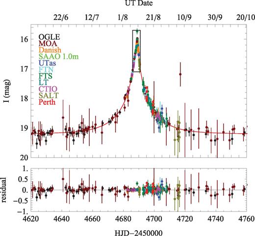
Data acquired with several telescopes (colour-coded) on gravitational microlensing event OGLE-2008-BLG-510 (MOA-2008-BLG-369) along with the best-fitting model light curve and the respective residuals. The region marked by the box is expanded in Fig. 2.

Open in new tabDownload slide

Figure 2

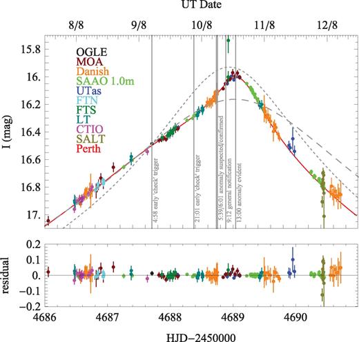
Data and model light curve for OGLE-2008-BLG-510 around the asymmetric peak. For comparison, we also show best-fitting model light curves for a single lens star using all data (short dashes) or data before triggering on the anomaly on 10 August 2008 (long dashes). Moreover, we have indicated the most relevant stages in the real-time identification of the anomaly.

Open in new tabDownload slide

Looking at the data and the model light curve, it seems in fact that the early triggers on 2008 August 9, spanning the region 4687.69 ≤ HJD − 245 0000.0 ≤ 4688.39 were due to a real anomaly, but its weakness together with the limited photometric precision and accuracy did not allow us to obtain sufficient evidence.

3 Data Reduction and Limitations by Systematics

The photometric analysis for this event posed several challenges. The source star was very faint (I∼ 19.23 according to OGLE data base) and heavily blended with a brighter companion. In fact, we found all data being affected by a scatter larger than what might be reasonably expected by the error bars assigned by the reduction software. A re-analysis of the images obtained from the FTN, LT, FTS, Danish 1.54 m, SAAO 1.0 m and Canopus 1.0 m telescope using dandia⁴ (Bramich 2008) made a crucial difference by removing previously present systematics which could have easily been mistaken as indications of higher order effects, and posed a puzzle in the interpretation of this event. dandia is an implementation of the difference imaging technique (Alard & Lupton 1998) whose specific power arises from modelling the kernel as a discrete pixel array, allowing us to properly deal with distorted star profiles because it makes no underlying assumptions about the shape of the point spread function (PSF).

While in frames with large seeing, the faint target star is not resolved from its companion, dandia manages to deliver separate photometric measurements for either of the stars, so that the blend ratio associated with our light curve is close to zero. However, for the worse frames, we are left with large noise and systematics. A saturated star was nearby, which was necessarily masked by our photometric pipeline, but which in turn placed constraints on the size of the PSF and the kernel that could be used during the image subtraction stage, particularly for the images that had high seeing values. In a few specific cases, using a larger fit radius would mean that the masked area around the saturated star fell within the fit radius of the source star, thereby reducing the number of pixels used in the photometry (Bramich et al. 2011). A new version that is currently under development discounts a bigger region of pixels around the saturated star from the kernel solution, since the kernel solution is most sensitive to contaminated pixels.

Shortly after the ongoing anomaly had been identified, the Moon was full and close to the target field of observation resulting in high sky background counts and a strong background gradient. While the pipeline can account for the latter, the former has an impact on the photometric accuracy that can be achieved. In fact, moonlight had a strong effect starting from 2008 August 11 (illumination fraction 80 per cent), when the Moon was ∼7°–10° from the target field, on to 2008 August 12 (illumination fraction 86 per cent), when it was ∼3°–7° from the target field. It was full on 2008 August 16. So, all the affected data were taken after the anomaly at the peak. Normally it is not advisable to observe if the Moon is bright and closer than 15° to the target. Obtaining a full characterization of the impact of Moon pollution on the photometry is not that straightforward to assess with difference imaging, because there are many other factors that affect the kernel solution as well, and the different contributions are not easy to isolate. We have however optimized our photometry to minimize the impact of Moon pollution and accounted for the uncertainty during our modelling runs. Moreover, dandia takes care of systematic effects by producing a χ² value for the star fits and reflecting these in the reported size of the photometric error bars.

Although all these efforts have strongly reduced the impact of systematic effects on the data taken during the descent, residual small trends are still visible in SAAO, Danish, FTS and LT data. These trends tend to drive the higher order orbital motion modelling searches towards artificious solutions (see Section 4.5). In the absence of better alternatives, we decide to keep these data points in the analysis because they provide important constraints to the basic parameters of the simpler models, but the search for higher order effects is substantially precluded.

4 Modelling

4.1 Microlensing light curves

Gravitational microlensing events show a transient brightening of an observed source star that results from the gravitational bending of its light by an intervening object, the ‘gravitational lens’. The gravitational microlensing effect of a body with mass M is characterized by the angular Einstein radius

(1)

where G is the universal gravitational constant, c is the vacuum speed of light and

(2)

is the relative parallax of the lens and source stars at distances D_L and D_S from the observer, respectively.

With source and lens stars separated by an angle u θ_E on the sky, the magnification becomes (Einstein 1936)

(3)

if we assume a uniform relative proper motion μ between lens and source star, the separation parameter u becomes

(4)

where t_E = θ_E/μ is the event time-scale, and the closest angular approach u₀ is realized at time t₀.

With F_S being the flux of the observed target star and F_B the background flux, the total observed flux becomes

(5)

with the baseline flux F_base=F_S+F_B and the blend ratio g=F_B/F_S, where

(6)

is the observed magnification.

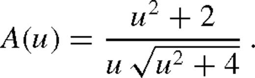
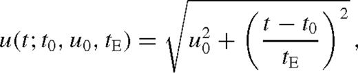
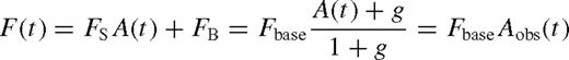
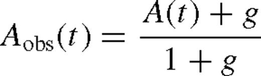
Because of A(u) monotonically increasing as u→ 0, ordinary microlensing light curves (due to a single point-like source and lens stars) are symmetric with respect to the peak at t₀, where the closest angular approach between lens and source u(t₀) = u₀ is realized and fully characterized by (t₀, u₀, t_E) and the set of (F_S, F_B) or (F_base, g) for each observing site and photometric passband. Best-fitting (F_S, F_B) follows analytically from linear regression, whereas the observed flux is non-linear in all other parameters.

4.2 Anomaly feature assessment and parameter search

Apparently, the only evident feature pointing to an anomaly in OGLE-2008-BLG-510 is the asymmetric shape of the peak (see Fig. 2). A comparison of the data with the best-fitting light curve at the time of the detection of the ongoing anomaly shows the strength of the effect, which becomes substantially more evident with the data observed on the falling side of the light curve, as also demonstrated by fitting an ordinary light curve to all data. Such weak effects can be explained by a finite extension of the central point caustic of a single isolated lens star due to binarity (which includes the presence of an orbiting planet). Moreover, the absence of further strong features excludes the source star from hitting or passing over the caustic. This straightforwardly restricts parameter space, and one could readily identify a limited number of viable configurations with regard to the topologies of the caustic and the source trajectory, and exclude all others. The use of an ‘event library’ where the most important features are stored had already been suggested by Mao & Di Stefano (1995), while generic features were the starting points for the exploration of parameter space in early efforts of modelling microlensing events (Dominik & Hirshfeld 1996; Dominik 1999a). Moreover, the identification of features for caustic-passage events has been proven powerful in efficient searches for all viable configurations (Albrow et al. 1999; Cassan 2008; Kains et al. 2009). More recent work built upon the universal topologies of binary-lens systems (Erdl & Schneider 1993) in order to classify light curves (Bozza 2001; Night, Di Stefano & Schwamb 2008). Based on the earlier work by Bozza (2001), we adopted an automated approach (Bozza et al. in preparation) that starts from 76 different initial conditions covering all possible caustic crossings and cusp approaches in all caustic topologies occurring in binary lensing (close, intermediate and wide; Erdl & Schneider 1993; Dominik 1999b). From these initial conditions, we have run a Levenberg-Marquardt algorithm for downhill fitting, and then we have refined the χ² minima by Markov chains.

The roundish shape of the peak, however, does not allow us to immediately dismiss the alternative hypothesis that the source rather than the lens is a binary system. Binary-source light curves are simply the superposition of ordinary light curves (Griest & Hu 1992), leading to a zoo of morphologies, which is however less diverse than that of binary lenses. Binary-lens systems can be uniquely identified from slope discontinuities and the sharp features that are associated with caustics, while smooth, weakly perturbed light curves may be ambiguous, and even potential planetary signatures might be mimicked by binary-source systems (Gaudi 1998).

4.3 Binary-lens models

In addition to its total mass M=M₁+M₂, a binary lens is fully characterized by the mass ratio q=M₂/M₁ of its constituents and, if one neglects the orbital motion, by their separation. The latter can be described by the dimensionless parameter d, where d θ_E is the angle on the sky between the primary and the secondary as seen from the observer. In contrast to a single lens, the microlensing light curve depends on the orientation of the source trajectory, where we measure the angle θ from the axis pointing from M₂ to M₁. As the reference point for the closest angular approach between lens and source, characterized by t₀ and u₀, we choose the centre of mass. This means that the source trajectory relative to the lens is described by

(7)

while the primary of mass M₁ is at the angular coordinate [dq/(1 +q), 0] θ_E and the secondary of mass M₂ at the angular coordinate [−d/(1 +q), 0] θ_E (see Fig. 3).

Figure 3

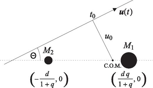
The geometry of a binary gravitational lens being approached by a single source star and the related parameters. The separation between the primary and the secondary is given by d, while the mass ratio is q=M₂/M₁. Positions on the sky arise from multiplying the dimensionless coordinates with the angular Einstein radius θ_E, so that t_E = θ_E/μ given an event time-scale, where μ denotes the absolute value of the relative proper motion between source and lens star.

Open in new tabDownload slide

Strong differential magnifications also result in the effects of the finite size of the source star on the light curve, quantified by the dimensionless parameter ρ_⋆, where ρ_⋆ θ_E is the angular source radius. We initially approximate the star as uniformly bright.

For the evaluation of the magnification for given model parameters, we have adopted a contour integration algorithm (Dominik 1995, 1998a; Gould & Gaucherel 1997) improved with parabolic correction, optimal sampling and accurate error estimates, as described in detail by Bozza (2010).

Our morphology classification approach leads to three viable configurations where the source trajectory approaches the caustic near the primary with different orientation angles, grazing one of the four cusps before having passed a neighbouring cusp at larger distance. We recover the well-known ambiguity between close and wide binaries (Griest & Safizadeh 1998; Dominik 1999b): all configurations come in two flavours. Fig. 4 illustrates these configurations, labelled ‘1’, ‘2’ and ‘3’, for the close-binary topology, whereas the wide-binary case is analogous. Given the symmetry of the binary-lens system with respect to the binary axis, there are three different cusps, one off-axis and two on-axis. For the off-axis cusp, there are two different neighbouring cusps, distinguishing models 2 and 3. In contrast, the neighbouring cusps to an on-axis cusp is the identical off-axis cusp, so that model 1 is not doubled up. In principle, there could be a solution near the approach of the other on-axis cusp, but this turned out not to be viable.

Figure 4

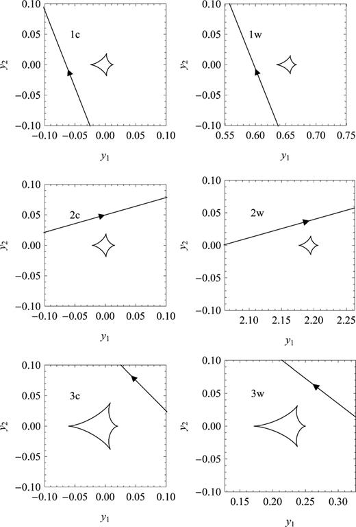
Illustration of the viable caustic and source trajectory configurations, showing how the trajectory approaches a cusp and passes with respect to the caustic. Models 1 and 2 differ in the exchanged roles of the on-axis and off-axis cusp, whereas models 2 and 3 exchange the on-axis cusp. Geometry and symmetry would allow for a fourth class of models, where the closest cusp approach is to the on-axis cusp on the side opposite the companion, but such were found not to be viable.

Open in new tabDownload slide

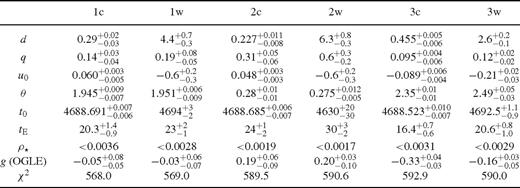
We end up with six candidate models that we label by 1c, 2c, 3c, 1w, 2w and 3w. The ‘c’ corresponds to the close-binary topology and the ‘w’ corresponds to the dual wide-binary topology. The values of the parameters of these models with their uncertainties are shown in Table 3. Model 1c comes with the smallest χ² (set equal to the number of degrees of freedom by rescaling the photometric uncertainties), with model 1w closely following with just Δχ²= 1. Models 2 and 3 come with Δχ²∼ 20, with model 2w being singled out by its wide parameter ranges. Models 1 prefer an OGLE blend ratio close to 0, whereas models 2 prefer a larger background, but are still compatible with zero blending. Models 3 come with a negative blend ratio. If one imposes a non-negative blend ratio, models 1 and 2 change rather little (see Table 4), but we did not find corresponding minima for the configurations of models 3, which rather tend towards models 2. Mass ratios q roughly span the range from 0.1 to 1. Given that the source passes too far from the caustic to provide significant finite-source effects, all models return only an upper limit on the source size parameter ρ_⋆. We will compare all models in detail in Section 4.6.

Table 3

Timeline of OGLE-2008-BLG-510 observations and anomaly detection.

Open in new tabDownload slide

Table 4

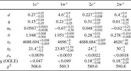
Viable static binary lens models with non-negative OGLE blend ratio imposed. While there is little effect on models and 2, models 3 have dropped out with no corresponding minima found.

Open in new tabDownload slide

4.4 Binary-source models

As anticipated, the binary source interpretation might be able to explain the anomaly in OGLE-2008-BLG-510 as efficiently as the binary lens. If we neglect the orbital motion, the microlensing light curve of a ‘static’ binary source with a single lens is just the superposition of two Paczyński curves with the same t_E, so that

(8)

where ω = F_{S, 2}/(F_{S, 1}+F_{S, 2}) is the flux offset ratio for the source fluxes F_{S, 1} and F_{S, 2}, and we just need to distinguish two pairs (u₁, t₁) and (u₂, t₂) that characterize the closest angular approach to each of the constituents.

As pointed out by Dominik & Hirshfeld (1996, appendix C), there is a two-fold ambiguity for the angular separation Δη between the source stars, given that the photometric light curve does not tell us whether they are on the same side (‘cis’ configuration) or on opposite sides (‘trans’ configuration) of the lens trajectory, where

(8)

The search in the parameter space is much simpler, since there is only one way of superposing two Paczyński curves so as to obtain the asymmetric peak of OGLE-2008-BLG-510. We found that a small negative blend ratio is preferred, where the parameters shift only very little if a non-negative blend ratio is enforced. The best-fitting model with this constraint is given in Table 5.

Table 5

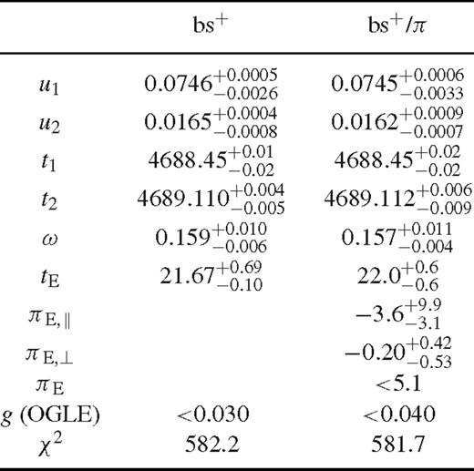
Binary-source model without and with parallax, where we constrain the OGLE blend ratio to be non-negative. The times t₁ and t₂ are in HJD - 245 0000, while all other parameters are dimensionless.

Open in new tabDownload slide

4.5 Higher order effects

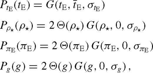
Beyond the basic static binary-lens and binary-source models presented above, we looked for the potential signatures of three possible higher order effects: annual parallax, lens orbital motion and source limb darkening.

As the Earth revolves around the Sun, the trajectory of the source relative to the lens system effectively becomes curved. The curvature depends on the orientation of the source trajectory relative to the ecliptic, which can be expressed by a parallax vector π_E (e.g. Gould 2004) with the absolute value

(10)

where the components (π_{E, ∥}, π_{E, ⊥}) parallel and perpendicular to the source trajectory characterize the relative direction of the ecliptic. A typical signature of the annual parallax effect in microlensing light curves is an asymmetry between the rise and the descent.

Starting from the static solutions of Table 4, we have run Markov chains including the two parallax parameters, where our results are summarized in Table 6. For models 1, χ² reduces by less than 1 with the two additional parameters, which shows the insignificance of parallax. There is a larger Δχ² for models 2, namely 7.3 and 2.5, respectively, but we need to consider that improvements at such level can easily be driven by data systematics (not following the assumption of uncorrelated normally distributed measurements). We therefore only use an upper limit on the parallax for constraining the physical nature of the lens system. Similarly, we do not find any significant parallax signal with the binary-source model (see Table 5) and a similarly weak limit.

Table 6

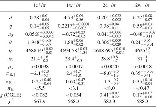
Models 1c⁺, 1w⁺, 2c⁺ and 2w⁺ including the annual parallax effect. The parameters are described in Table 3, with the addition of the parallax parameters π_E,∥ and π_E,⊥ For the total parallax pE we give the upper limit at 68 per cent confidence level.

Open in new tabDownload slide

The orbital motion of the lens might particularly affect our candidate models in close-binary topology, where a relatively short orbital period compared to the event time-scale t_E is possible and worth being checked for. We have therefore performed an extensive search for candidate orbital configurations, including the three velocity components of the secondary lens in the centre of mass frame as additional parameters. Due to the lack of evident signatures of orbital motion, we have just considered circular orbits, which are completely determined by the three parameters just introduced. Indeed, we find particular solutions with a sizeable improvement in the χ² with respect to all static models. For example, model 1c gets down to χ²= 539. However, a closer look at the candidate solutions thus found shows that they are actually fitting the evident systematics in the data taken during the descent of the microlensing light curve, when the Moon was close to the source star (see the discussion in Section 3). In all these data, a weak overnight trend is present, whose steepness depends on the particular image reduction pipeline employed. Again, we see that systematics in the data prevent us from drawing firm conclusions just from improvements in χ², not knowing whether the data related to it show a genuine signal. Consequently, we will withdraw the hypothesis that orbital motion can be detected, and we will not use any orbital motion information in the interpretation of the event.

We have also looked into source orbital motion, and not that surprisingly, we also find that the fit is driven by systematic trends of the data over the night. Therefore, we will not consider the improvement in the χ² down to 544 as due to intrinsic physical effects.

Finally, we have tested several source brightness profiles to account for limb darkening for all models, but the difference with the uniform brightness models is tiny, orders of magnitude smaller than the photometric uncertainty. This is consistent with the fact that in all models the source passes relatively far from the caustic, leaving no hope to study the details of the source structure.

4.6 Comparison of models

For the peak region, the differences between the models remain below 2.5 per cent (see Fig. 5), which make these difficult to probe with the apparent scatter of the data. Moreover, only if it is ensured that systematic effects are consistently substantially below this level, will a meaningful discrimination between the competing models be possible. In our opinion, this poses the most substantial limit to our analysis, and we therefore abstain from drawing very definite conclusions about the physical nature of the OGLE-2008-BLG-510 microlens. Fig. 5 also shows that the differences between the respective pairs of close- and wide-binary models are even much smaller, less than 0.4 to 0.7 per cent over the peak. It can also be seen that models are made to coincide better in the peak region where more data have been acquired, as compared to the wings where larger differences of 3–6 per cent are tolerated.

Figure 5

Observable magnitude shift Δm = 2.51g{[A(t) + g]/(1 + g)} as a function of time for all suggested models as compared to model 1c. The OGLE blend ratio has been used as reference.

Open in new tabDownload slide

As Fig. 6 shows, the differences between the models with respect to the residuals with observed data appear to be rather subtle. Additional freedom that makes them less distinguishable arises from adopting a blend ratio for each of the sites and each of the models, allowing for different relations between the blend ratios among the models. A successful fit should be characterized by data falling randomly to both sides of the model light curve. For model 1, we find all Canopus 1.0 m data taken in the time range 4689.5 ≤ HJD − 245 0000 ≤ 4690.5 to be above the model light curve, whereas these are distributed to both sides with models 2. On the other hand, models 2 introduce a trend in some SAAO data over the peak that does not show with other models. We also see that models 3 are more closely related to models 2 than to models 1, with rather similar behaviour over the peak, while the differences in the wing regions are related to the different blend ratios. In fact, both models 2 and 3 have the second and closer cusp approach to the off-axis cusp, whereas the roles of the on-axis and off-axis cusps are flipped for models 1.

Figure 6

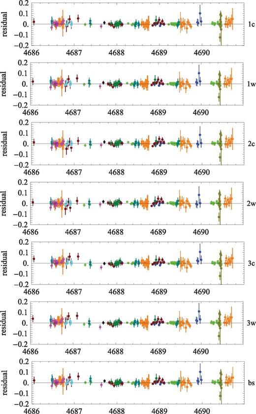
Residuals in the peak region of OGLE-2008-BLG-510 for all proposed models.

Open in new tabDownload slide

It is also very instructive to look at Δχ² between the models as a function of time as the data were acquired (see Fig. 7), which obviously depends on the sampling. While models 3 as well as the binary-source model rather gradually lose out to models 1 for 4683 ≤ HJD − 245 0000 ≤ 4691, models 2 perform much worse than all other models for the rather short period 4688.0 ≤ HJD − 245 0000 ≤ 4689.5, which happens just to coincide with the skewed peak. However, for 4686.0 ≤ HJD − 245 0000 ≤ 4688.0 and 4689.5 ≤ HJD − 245 0000 ≤ 4690.5, models 2 do a better job than models 1. It is in the nature of χ² minimization that more weight is given to regions with a denser coverage by data. As a consequence, relative χ² between competing regions of parameter space depend on the specific sampling. In fact, the region 4689.5 ≤ HJD − 245 0000 ≤ 4690.5 which favours model 2 has a sparser coverage than preceding nights. Moreover, we find model 3c outperforming all other models for 4645 ≤ HJD − 245 0000 ≤ 4682, but this is given little weight. The weight arising by the sampling is particularly a relevant issue given that for non-linear models, the leverage to a specific parameter strongly depends on the time observations are taken. We immediately see that there is an extreme danger of conclusions being driven by systematics in a single data set during a single night, potentially overruling all that we learn from other data.

Figure 7

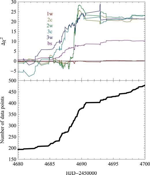
Δχ² as a function of time for all suggested models relative to model 1c, along with the cumulative number of data points up to that time.

Open in new tabDownload slide

5 Physical Interpretation

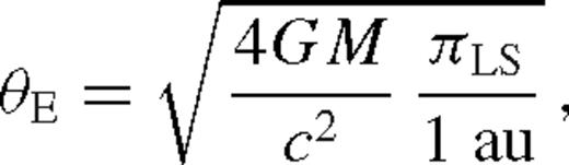
An ordinary microlensing event is determined by the fluxes of the source star F_S and the blend F_B, the mass of the lens star M, the source and lens distances D_S and D_L, as well as the relative proper motion μ between lens and source star (or the corresponding effective lens velocity v=D_L μ), and finally the angular source-lens impact θ₀ and its corresponding epoch t₀. However, the photometric light curve is already fully described by a smaller number of parameters. Apart from F_S and F_B, it is completely characterized by t₀, u₀=θ₀/θ_E and t_E=θ_E/μ, where the angular Einstein radius θ_E, as given by equation (1) absorbs M, D_L and D_S. All the physics of D_S, D_L, M and v gets combined into the single model parameter t_E, and information about the detailed physical nature gets lost.

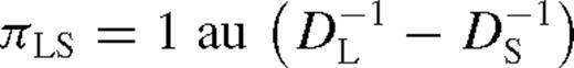
Higher-order effects can play an important role in recovering the information. Additional relations between the physical properties can be established if the light curve depends on further parameters that are related to the angular Einstein radius θ_E or the relative lens-source parallax π_LS. In particular, finite-source effects with the parameter ρ_⋆ = θ_⋆/θ_E or annual parallax with the microlensing parallax π_E = π_LS/θ_E allow solving for D_L, M and v, once D_S and the angular size θ_* of the source star can be established. Moreover, as in the case of OGLE-2008-BLG-510 here, even the absence of detectable effects can provide valuable constraints to parameter space. In fact, as discussed in the previous section, the anomaly of OGLE-2008-BLG-510 is almost indifferent to the source radius. Moreover, no parallax signal is clearly detected in either model. Finally, our attempts to find solutions with orbital motion just bumped into systematic overnight trends in the data.

But even if the physical properties of the lens system cannot be determined directly, Bayes' theorem provides a means of deriving their probability density. In fact, with the physical properties ψ and the model parameters p, one finds a probability density P_ψ(ψ|p) of ψ given p as

(11)

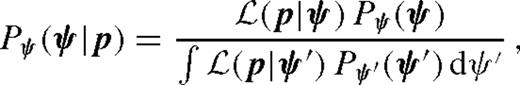
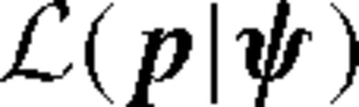where P_ψ(ψ) is the prior probability density of the physical properties ψ and is the likelihood for the parameters p to arise from the properties ψ.

While prior probability densities P_ψ(ψ) for the physical properties are straightforwardly given by a kinematic model of the Milky Way and mass function of the various stellar populations, the likelihood is proportional to the differential microlensing rate d^kΓ/(dp₁…dp_k) (cf. Dominik 2006), which is to be evaluated using the constraining relations between the model parameters p and the physical properties ψ. We determine P_ψ(ψ) following the lines of Dominik (2006). While Calchi Novati et al. (2008) have recently discussed Galactic models in some detail, we basically follow the choice of Grenacher et al. (1999). In particular, we consider candidate lenses in an exponential disc or in a bar-shaped bulge. The respective mass functions are taken from Chabrier (2003). In absence of comprehensive data on binary systems, we simplify our estimate by referring to the total mass of the system. The only difference with respect to Dominik (2006) is that we consider an anisotropic velocity dispersion for stars in the bulge (Han & Gould 1995), with σ = (116, 90, 79) km s⁻¹ along the three bar axes defined therein. Actually, this difference does not have any major effect on the final result. The denominator in equation (11) just reflects that the probability density is properly normalized, i.e. , which can be achieved trivially.

In addition to the information contained in the event time-scale t_E, we also take into account the constraints arising from the upper limits on the source size, the parallax and the luminosity of the lens star, as given by the blend ratio g, where we neglect the secondary, and only consider the mass of the primary in the mass–luminosity relation.

The angular source radius θ_⋆ can be measured using the technique of Yoo et al. (2004). The dereddened colour and magnitude of the source are measured from an instrumental colour–magnitude diagram as [(V−I), I]_{0, S}= (0.63, 17.78), where we assumed that the clump centroid is at [(V−I)₀, M_I]_clump = (1.06, −0.10) (Bensby et al. 2011, Nataf private communication), the Galactocentric distance is R₀= 8.0 kpc and the clump centroid lies 0.2 mag closer to us than the Galactic Centre, since the field is at Galactic latitude l = +5°.2. Therefore, we also set D_S = 7.3 kpc. We then convert from V/I to V/K using the colour–colour relations of Bessell & Brett (1988). Finally, we use the V/K colour/surface–brightness relation of Kervella et al. (2004) to obtain θ_⋆= (0.80 ± 0.06) μ as.

Rather than just basing our analysis on the best-fitting values, we also take into account the model parameter uncertainties. From our Markov chain Monte Carlo runs, we find that t_E, ρ_⋆, π_E and g (OGLE) are basically uncorrelated. Their combined probability can therefore fairly be approximated by the product of the individual probability densities

(12)

We approximate each of these distributions by a Gaussian

(13)

where

(14)

with the dispersions of these Gaussians being identified with the 68 per cent confidence limits listed in Table 6.

We find a probability density in D_L, M and v. By integrating over v, and changing from M to log M, we obtain a probability density in the (D_L, log M) plane. In this integration, as explained by Dominik (2006), the dispersion in the Einstein time is practically irrelevant and we can approximate the t_E distribution by a delta function. The arising posterior probabilities are illustrated in Fig. 8 separately for the disc and bulge lenses for models 1 and 2. We can appreciate the small difference between the close- and wide-binary models (whose contours are dashed in Fig. 8). The wide topology slightly favours a smaller distance and a higher mass for the lens system. Higher masses are cut off by the blending constraint, as the lens would become too bright to be compatible with the absence of blending. In fact, this blending constraint readily dismisses models 3. The source radius constraint slightly cuts small lens masses as these would yield a too small Einstein radius. Finally, only the tail of the disc distribution at small D_L is affected by the parallax constraint.

Figure 8

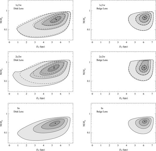
Contours of the probability density containing 95, 68, 38 and 10 per cent probability in the mass–distance plane for the lens in binary-lens models 1 (top), binary-lens models 2 (middle) and the binary-source model (bottom). The panels on the left treat the case of a disc lens, while those on the right consider a bulge lens. The dashed lines are the contours for models 1w and 2w, respectively. The filled (empty) circles are the modes of the probability density for the close- (wide-)binary models.

Open in new tabDownload slide

The relative weight of disc and bulge for each microlensing model is obtained by integrating these distributions over the whole (D_L, log M) plane. Table 7 shows the probabilities for each microlensing model and each hypothesis for the lens population. We also show the average lens distance and mass in each case. We find that the cut on higher masses due to the absence of blending significantly penalizes the bulge, which is known to have a higher microlensing rate (Kiraga & Paczyński 1994; Dominik 2006). This fact witnesses how the information coming from the study of our specific microlensing event effectively selects the viable lens models.

Table 7

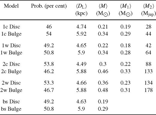
Expectation values of lens distance D_L and lens mass M for the different binary-lens models, and assessment of probability for the lens to reside in the Galactic disc or bulge.

Open in new tabDownload slide

Within the parameter uncertainties of the binary-lens models, there is some significant overlap in the possible physical nature of the lens system (with model 2w being compatible with a very wide range). We find that an M dwarf orbited by a brown dwarf appears to be a favoured interpretation, but we cannot fully exclude a more massive secondary. Regardless of the specific model, a location in the Galactic disc appears to be as plausible as in the Galactic bulge. The microlensing light curve does not definitely clarify whether the system is in a wide or in a close configuration because of the well-known degeneracy of the central caustic. It is interesting to note that if we use the average values for the total mass and the distance we can estimate that the minimum value for the orbital period in model 1c (1w) is 296 d (51 yr) with a minimum orbital radius of 0.52 (8.25) au. Even in the closer configuration, detecting any orbital motion signal in this event would have been quite difficult. This also reinforces our rejection of all models with very short orbital periods found during the modelling phase.

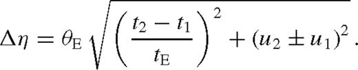
For the binary-source model, we find with the I-band magnitude and the luminosity offset ratio ω, the masses of the two components as m₁ = 1.03 and m₂ = 0.80 M_⊙. The V−I index of this system is 0.1 mag larger than the V−I index of a single source that would yield all the observed flux. Moreover, by adopting values for the lens mass and distance in the middle of the two averages for the bulge or disc hypothesis (see Table 7), the physical size of the angular Einstein radius θ_E at the source distance D_S becomes D_Sθ_E= 2.35 au. For a face-on circular orbit, we therefore find the orbital radius simply as r₀=D_SΔη, where Δη as given by equation (9) denotes the angular separation between the binary-source constituents. With the total mass of the binary-source system m=m₁+m₂∼ 1.83 M_⊙, we then obtain orbital periods of P_{0, cis}∼ 16d or P_{0, trans}∼ 29 d for the cis- or trans-configurations, respectively. For an orbital inclination i, the orbital radius increases as r=r₀/(cos i), so that the orbital periods increase as P = P₀/(cos i)^3/2. For orbits with an eccentricity ɛ, the observed separation r is limited to the range a(1 −ɛ) ≤r≤a(1 +ɛ), where a denotes the semimajor axis. While r=a for a circular orbit, one finds in particular a≥r/2. Therefore, in the general case, orbital periods still have to fulfil P≥P₀/(2 cos i)^3/2. Given both the small colour difference and a plausibly long orbital period (as compared to the event time-scale of t_E∼ 22 d), there is no apparent inconsistency within the proposed binary-source model.

6 Conclusions

So far, most of the results arising from gravitational microlensing campaigns have been based on the detailed discussion of individual events that show prominent characteristic features that allow unambiguous conclusions on the underlying physical nature of the lens system that caused the event. However, with its sensitivity to mass rather than light, gravitational microlensing is particularly suited to determine population statistics of objects that are undetectable by any other means. This not only includes planets in regions inaccessible to other detection techniques, but also brown dwarfs, low-mass stellar binaries and stellar-mass black holes. Meaningful population statistics will only arise from controlled experiments with well-defined deterministic procedures, and similarly the data analysis needs to adopt a homogeneous scheme. Given that the information arises from the constraints posed by the data on parameter space, i.e. what can be excluded rather than what can be detected, events with weak and potentially ambiguous features need to be dealt with appropriately.

The event OGLE-2008-BLG-510, which was subject to a detailed analysis in this paper, is a rather typical representative of the large class of events with evident weak features. Our light-curve morphology classification approach revealed that the apparent asymmetric shape of the peak appears to be compatible with a range of binary-lens models or a binary-source model. A particular challenge in the interpretation of the acquired data is dealing with systematic effects that can lead to the misestimation of measurement uncertainties, non-Gaussianity and correlations. This in turn strongly limits the validity of the application of statistical techniques that assume uncorrelated and normally (Gaussian) distributed data. We moreover find that the sampling of microlensing light curve affects the preference of regions of parameter space, and that conclusions therefore are at risk to be driven by systematics in the data rather than real effects. In the specific case of OGLE-2008-BLG-510, all suggested models coincide within 2.5 per cent in the peak region (where the sampling is dense), and in order to discriminate, not only does the scatter of the data need to be small, but more importantly, systematics need to be understood or properly modelled to a level substantially below the model differences. For OGLE-2008-BLG-510, we found that systematic trends in some data sets simulate a fake scale for orbital motion, which (if present) is hidden below systematics and thus impossible to determine.

Despite the fact that the viable binary-lens models differ in the geometry between the binary-lens system and the source trajectory, there is some overlap in the resulting physical nature of the binary-lens system, taking into account the model parameter uncertainties. In fact, we find the lens system consisting of an M dwarf orbited by a brown dwarf a favourable interpretation, albeit that we cannot exclude a different nature.

The large number of microlensing events with weak features are currently waiting for a comprehensive statistical analysis, and lots of interesting results are likely to be buried there. It however requires a very careful analysis of the noise effects in the data as well as modelling techniques that map the whole parameter space rather than just finding a single optimum, which is just a point estimate, and moreover biased if χ² minimization is used.⁵ Currently, we neither understand the paucity of reported events due to a binary source nor the impact of brown dwarfs on microlensing events, and we might even need to look into weak signatures and their statistics in order to arrive at a consistent picture.

The detection of the weak microlensing anomaly in OGLE-2008-BLG-510 also demonstrated the power and feasibility of automated anomaly detection by means of immediate feedback, i.e. requesting further data from a telescope which is automatically reduced and photometric measurements being made available within minutes. This is an important step in the efficient operation of a fully deterministic campaign that gets around the involvement of humans in the decision chain and offers the possibility to derive meaningful population statistics by means of simulations.

Acknowledgments

The Danish 1.54 m telescope is operated based on a grant from the Danish Natural Science Foundation (FNU). The ‘Dark Cosmology Centre’ is funded by the Danish National Research Foundation. Work by C. Han was supported by a grant of National Research Foundation of Korea (2009-0081561). Work by AG was supported by NSF grant AST-0757888. Work by BSG, AG and RWP was supported by NASA grant NNX08AF40G. Work by SD was performed under contract with the California Institute of Technology (Caltech) funded by NASA through the Sagan Fellowship Program. The MOA team acknowledges support by grants JSPS20340052, JSPS20740104 and MEXT19015005. Some of the observations reported in this paper were obtained with the Southern African Large Telescope (SALT). LM acknowledges support for this work by research funds of the International Institute for Advanced Scientific Studies. MH acknowledges support by the German Research Foundation (DFG). TCH is funded through the KRCF Young Scientist Research Fellowship Programme. CUL acknowledges support by Korea Astronomy and Space Science Institute (KASI) grant 2012-1-410-02. DR (boursier FRIA) and JSurdej acknowledge support from the Communauté française de Belgique – Actions de recherche concertées – Académie universitaire Wallonie-Europe. The OGLE project has received funding from the European Research Council under the European Community's Seventh Framework Programme (FP7/2007-2013) /ERC grant agreement no. 246678. Dr David Warren provided support for the Mt Canopus Observatory. MD, YT, DMB, CL, MH, RAS, KH and CS are thankful to Qatar National Research Fund (QNRF), member of Qatar Foundation, for support by grant NPRP 09-476-1-078.

References

Author notes