Isolated starless cores in infrared dark clouds in the Hi-GAL survey

Abstract

1 INTRODUCTION

Infrared dark clouds (IRDCs) were initially discovered by the Midcourse Space Experiment (Carey et al. 1998; Egan et al. 1998) and Infrared Space Observatory (Perault et al. 1996) surveys as dark regions against the mid-infrared (MIR) background. The densest IRDCs may eventually form massive stars (Kauffmann & Pillai 2010) and are therefore presumed to represent the earliest observable stage of high-mass star formation.

Some IRDCs contain cold, compact condensations called infrared dark cores, also referred to as ‘clumps’ (e.g. Battersby et al. 2010) or ‘fragments’ (e.g. Peretto & Fuller 2009). The most massive of these objects are believed to be the high mass equivalent of low-mass pre-stellar cores (Ward-Thompson et al. 1994; Carey et al. 2000; Redman et al. 2003; Garay et al. 2004).

Observations of IRDCs have shown them to have low temperatures (T < 25 K; e.g. Egan et al. 1998; Teyssier, Hennebelle & Perault 2002), high densities (n_H >10⁵ cm⁻³; Carey et al. 1998, 2000; Egan et al. 1998) and masses between ∼10²–10⁴ M_⊙ (Rathborne et al. 2005; Ragan, Bergin & Gutermuth 2009).

Within the IRDCs, infrared dark cores have been observed with radii ranging from 0.04 to 1.6 pc, masses from 10 to 1000 M_⊙ and densities from 10³ to 10⁷ cm⁻³ (Garay et al. 2004; Ormel et al. 2005; Rathborne et al. 2005; Rathborne, Jackson & Simon 2006; Swift 2009; Zhang et al. 2011). This is consistent with them being the precursors to hot molecular cores, the next observable stage in high-mass star formation (Rathborne et al. 2006).

Using CO velocities, kinematic distances have been calculated for several hundred IRDCs and, by extension, their cores (Simon et al. 2006; Jackson et al. 2008). The distribution of IRDCs in the first Galactic quadrant differs from those in the fourth quadrant. In the first quadrant, IRDCs have a mean Galactocentric distance of ∼5 kpc (Jackson et al. 2008), whereas those in the fourth quadrant are typically found at ∼6 kpc (Peretto & Fuller 2010). This suggests that many IRDCs may be located in the Scutum–Centaurus spiral arm. The association of IRDCs with a spiral arm lends weight to the theory that IRDCs are the birthplace of high-mass stars (Jackson et al. 2008).

Cores within IRDCs can be separated into different classes based on observational parameters. Starless cores, also called ‘quiescent cores’, are the youngest subset of infrared dark cores. They are not yet undergoing any form of active star formation and so contain no MIR activity (Chambers et al. 2009). As the cores evolve, they leave the starless phase and begin to exhibit tracers of star formation, first 24-m emission, and then PAH 8-m emission (see Wilcock et al. 2012 for more details). When the cores have reached the latter stage, they are thought to contain a hyper- or ultra-compact H ii region (Chambers et al. 2009; Battersby et al. 2010).

In a previous paper (Wilcock et al. 2012), we used data from the Herschel Infrared Galactic Plane Survey (Hi-GAL; Molinari et al. 2010a,b) to observe the IRDCs from Peretto & Fuller (2009)– hereafter PF09 – at far-infrared (FIR) wavelengths. We identified 1205 IRDCs that were simultaneously Spitzer-dark in the MIR and Herschel-bright in the FIR, and found that 972 of them contained identifiable cores, as defined by peaks in their FIR emission at 250 m. We classified the cores depending on the presence or absence of an embedded MIR source at 8 or 24 m. We identified the youngest, least-evolved cores as those which contained no embedded MIR point sources, and labelled them starless. We found 170 IRDCs containing starless cores.

Previous study has shown that high-mass star formation is unlikely to have already occurred in starless cores (Wilcock et al. 2011). However, it should be noted that if the column density were high enough, it is possible for an IRDC to absorb the MIR emission from more evolved cores and appear starless despite the presence of embedded protostars (Pavlyuchenkov et al. 2011).

In this paper, we identify the most isolated of these 170 starless cores, based on their appearance at FIR wavelengths. We find 20 starless cores that satisfy our conditions for being the most isolated. We then model these 20 cores to determine their physical parameters.

2 DATA

The Herschel1 Space Observatory was launched in 2009 May. Herschel carries three science instruments. These are the Spectral and Photometric Imaging Receiver (SPIRE; Griffin et al. 2010); the Photodetector Array Camera and Spectrometer (PACS; Poglitsch et al. 2010) and the Heterodyne Instrument for the Far Infrared (HIFI; de Graauw et al. 2010). Herschel is capable of observing in the FIR between 55 and 671 m. Here, we only use data from SPIRE and PACS.

The data used in this paper were taken as part of the Hi-GAL, an Open Time Key Project of the Herschel Space Observatory (Molinari et al. 2010a,b). The Hi-GAL aims to perform a survey of the Galactic plane using the PACS and SPIRE instruments. The two are used in parallel mode to map the Milky Way Galaxy simultaneously at five wavelengths (70, 160, 250, 350 and 500 m), with resolution up to 5 arcsec at 70 m.

PACS data reduction was performed using the Herschel Interactive Pipeline Environment (HIPE; Ott 2010), with some additions described by Poglitsch et al. (2010). The standard deglitching and crosstalk correction were not used and custom procedures were written for drift removal (Traficante et al. 2011).

SPIRE data processing used the standard processing methods (Griffin et al. 2010), with both standard deglitching and drift removal. In both cases, the ROMAGAL generalized least-squares algorithm (Traficante et al. 2011) was used to produce the final maps. A more detailed discussion of the data reduction process is given by Traficante et al. (2011).

We also make use of 8-m and 24-m data from Spitzer2 that were taken as part of the Galactic Legacy Infrared Mid-Plane Survey Extraordinaire (Benjamin et al. 2003) and MIPSGAL (Carey et al. 2009), respectively. We used the mosaics available from the Spitzer Science Centre to create 8- and 24-m maps of the region 300°≤l≤ 330° and |b|≤ 1°.

3 SOURCE SELECTION AND MODELLING

3.1 Source sample

We took as our initial sample the 170 IRDCs with starless cores identified by Wilcock et al. (2012). A Gaussian profile was fitted to the 250-m intensity of each core. This was used to determine the full width half-maximum (FWHM) of the core. Each starless core was also studied at 160 and 500 m to determine if it was isolated. Our model is best suited to isolated cores because isolated cores are more likely to have the simple internal structures.

For a core to be deemed isolated, it has to be unconfused by a neighbouring core within the IRDC. We defined this by saying that there must be a minimum depth of magnitude greater than 3σ between the peak of one core and that of any neighbouring core. This must be true at all FIR wavelengths (160, 250, 350 and 500 m). Of the 170 IRDCs with starless cores, only 20 cores were found to be truly isolated according to our rigorous definition. These cores are listed in Table 1.

3.2 Distances

The distances to our infrared dark cores had not been previously calculated. The galactocentric distance to each core was therefore estimated using the Brand & Blitz (1993) velocity curve

1

where a₁= 1.0069, a₂= 0.0363 and a₃= 0.0065 in the fourth quadrant of the Galactic plane. θ is the core’s orbital velocity and d_g is its Galactocentric distance. θ₀ and d_g,0 are the solar equivalents. Canonical values of 8.5 kpc and 220 km s⁻¹ were used for d_g,0 and θ₀, respectively. CO velocities were taken from Dame et al. (1987). This method is only accurate up to 8 kpc (Brand & Blitz 1993).

From this, the heliocentric distance was calculated using

2

where d_h is the core’s heliocentric distance and b and l are the Galactic latitude and longitude of the core, respectively. This is solved as a quadratic equation and results in two possible distances for each core – one on the nearside of the Galaxy and one on the farside.

The near/far distance ambiguity exists in all cases. However, each of our cores had to show up in absorption at 8 m to be considered a candidate IRDC in the first place (PF09). Therefore, most of the MIR-emitting material must be behind our cores, rather than in front of them, or absorption would not be evident. For this reason, we assume that the near distance is correct for all of the cores. The calculated distance to each core is listed in Table 1.

Fourth quadrant IRDCs have a typical galactocentric distance of 6 kpc (Jackson et al. 2008) and a typical heliocentric distance of 4 kpc (Peretto & Fuller 2010). The mean heliocentric distance to our isolated cores is 3.1 kpc, closer than 4 kpc. This is due to a selection bias in our isolation criterion. It can be seen in Fig. 1, where we compare the masses (see the discussion below) and radii of the cores to their distance. Only cores with a high mass or large radius were seen as isolated at greater distances. This is due to the annular resolution of Herschel. Using our lowest data points, a cutoff is extrapolated. This is shown as a dashed line in Fig. 1. Below this cutoff, a core is unlikely to be selected for modelling due to our isolation criterion.

Figure 1

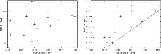
Mass (left) and radius (right) versus core heliocentric distance. The dashed line shows the cutoff point for a core’s radius – a core with a radius below this line will not have been selected for modelling due to our ‘isolated’ criterion (see the text).

Open in new tabDownload slide

3.3 Radiative transfer modelling

Our 20 isolated, starless cores were modelled using phaethon (Stamatellos & Whitworth 2003, 2005; Stamatellos et al. 2010). phaethon is a three-dimensional Monte Carlo radiative transfer code. The code uses luminosity packets to represent the ambient radiation field in the system. These packets are injected into the system where they interact (are absorbed, re-emitted or scattered) stochastically.

The input variables of the code are the density profile, the strength of the interstellar radiation field (ISRF), the dust properties of the system, the size of the core and its geometry (i.e. spherical, flattened or cometary). The code calculates the temperature profile of the system as well as spectral energy distributions (SEDs – see Fig. 2) and intensity maps, at different wavelengths and viewing angles – see Appendix A.

Figure 2

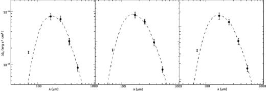
Example SEDs for cores 307.495+0.660, 318.573+0.642 and 322.334+0.561. The points show the observed fluxes at each of our wavelengths and the model SED is shown as a dashed line. The 70-m data provide upper limits only.

Open in new tabDownload slide

phaethon uses Ossenkopf & Henning (1994) opacities for a standard Mathis, Rumpl & Nordsieck (1977) grain mixture of 52 per cent silicate and 47 per cent graphite with grains that have coagulated and accreted thin ice mantles over 10⁵ yr at densities of 10⁶ cm⁻³. Further details of the dust model used can be found in Stamatellos & Whitworth (2003, 2005) and Stamatellos et al. (2010).

All the cores showed some measure of eccentricity in the observations and so were modelled with a flattened geometry – see Stamatellos et al. (2004, 2010) for details. In this case, the density profile is given by

3

where r is the radial distance, θ is the polar angle and R₀ is the flattening radius (i.e. the radial distance for which the central density is approximately constant) and was set to one-tenth of the core’s semimajor axis, R_max. n₀(H₂) is the central density, which is controlled as an input variable. A is the asymmetry factor and controls the equatorial to polar optical depth ratio and determines how flattened the core is (i.e. its eccentricity). p determines how quickly the optical depth changes from equator to pole, and was set to 2. These values for R₀ and p were chosen as they have been shown previously to give sensible results when modelling cold cores (e.g. Stamatellos et al. 2010; Wilcock et al. 2011). By restricting these parameters to sensible estimates, a single model may be fitted to each core.

The size and shape of each modelled core were set to match the observed core at 250 m. R_max was set equal to the FWHM of the major axis of each observed core. The R_max of each core is listed in Table 1. The FWHMs of the cores have an error of ±15 per cent, primarily due to uncertainties in the background levels. Contours from the 250-m observations were overlaid on to images of the modelled core. The asymmetry factor of each model was manually varied until the modelled shape visually matched that of the observed core.

To test the goodness of fit of the modelled morphology to the observed morphology, we compared the eccentricity and the FWHM. For the eccentricity, a percentage difference of less than 20 per cent was considered a good fit. The eccentricities of the observed and modelled cores are given in Table 2. The FWHM of the modelled core is expected to agree with the FWHM of the observed core within the prescribed errors of ∼15 per cent. The FWHMs of the observed and modelled cores at 250 m are given in Table 3. Differences between the model and observed morphology are mainly due to the assumption that the observed cores were perfect ellipses and the difficulties of fitting such a model by eye.

Table 3

Open in new tab

The FWHM of the cores at 250 m. Column 2 gives the FWHM when measured from the data and column 3 shows the FWHM as measured from the model. Both have errors of ±15 per cent. See the text for details.

IRDC name	FWHM at 250 m (arcsec)
	Observed	Model
305.798−0.097	62	82
307.495+0.660	55	59
309.079−0.208	57	65
309.111−0.298	38	43
310.297+0.705	45	38
314.701+0.183	40	45
318.573+0.642	40	44
318.802+0.416	45	45
318.916−0.284	38	42
321.678+0.965	65	72
321.753+0.669	85	79
322.334+0.561	55	63
322.666−0.588	42	40
322.914+0.321	38	42
326.495+0.581	33	39
326.620−0.143	73	73
326.632+0.951	24	31
326.811+0.656	43	43
328.432−0.522	58	57
329.403−0.736	47	51

IRDC name	FWHM at 250 m (arcsec)
	Observed	Model
305.798−0.097	62	82
307.495+0.660	55	59
309.079−0.208	57	65
309.111−0.298	38	43
310.297+0.705	45	38
314.701+0.183	40	45
318.573+0.642	40	44
318.802+0.416	45	45
318.916−0.284	38	42
321.678+0.965	65	72
321.753+0.669	85	79
322.334+0.561	55	63
322.666−0.588	42	40
322.914+0.321	38	42
326.495+0.581	33	39
326.620−0.143	73	73
326.632+0.951	24	31
326.811+0.656	43	43
328.432−0.522	58	57
329.403−0.736	47	51

Table 3

Open in new tab

The FWHM of the cores at 250 m. Column 2 gives the FWHM when measured from the data and column 3 shows the FWHM as measured from the model. Both have errors of ±15 per cent. See the text for details.

IRDC name	FWHM at 250 m (arcsec)
	Observed	Model
305.798−0.097	62	82
307.495+0.660	55	59
309.079−0.208	57	65
309.111−0.298	38	43
310.297+0.705	45	38
314.701+0.183	40	45
318.573+0.642	40	44
318.802+0.416	45	45
318.916−0.284	38	42
321.678+0.965	65	72
321.753+0.669	85	79
322.334+0.561	55	63
322.666−0.588	42	40
322.914+0.321	38	42
326.495+0.581	33	39
326.620−0.143	73	73
326.632+0.951	24	31
326.811+0.656	43	43
328.432−0.522	58	57
329.403−0.736	47	51

IRDC name	FWHM at 250 m (arcsec)
	Observed	Model
305.798−0.097	62	82
307.495+0.660	55	59
309.079−0.208	57	65
309.111−0.298	38	43
310.297+0.705	45	38
314.701+0.183	40	45
318.573+0.642	40	44
318.802+0.416	45	45
318.916−0.284	38	42
321.678+0.965	65	72
321.753+0.669	85	79
322.334+0.561	55	63
322.666−0.588	42	40
322.914+0.321	38	42
326.495+0.581	33	39
326.620−0.143	73	73
326.632+0.951	24	31
326.811+0.656	43	43
328.432−0.522	58	57
329.403−0.736	47	51

The flux density, integrated over twice the FWHM of each core using an elliptical aperture, was measured in all five FIR maps and an SED was plotted. These flux densities have been background subtracted, where the background was defined using an off-cloud, elliptical aperture.

The central density, n₀(H₂), and the ISRF incident on the cores were manually varied until the output model’s SED matched the observed data. The ISRF is taken to be a multiple of a modified version of the Black (1994) radiation field, which gives a good approximation to the radiation field in the solar neighbourhood. The final values for n₀(H₂) and the incident ISRF have an uncertainty of ±15 per cent. This is based on a by-eye estimation of how much they can be varied until the model SED no longer fits the observed flux densities. Examples of the model SEDs are shown in Fig. 2 as a dotted line. The final values for n₀(H₂) and the incident ISRF are listed in Table 1.

To test the goodness of fit of the modelled SED to the observed SED, the χ² value was calculated for each core. Only the flux densities from 160 to 500 m were taken into account when calculating χ². The 70 m point was only used as an upper limit and was ignored in this calculation. R_max and the asymmetry factor were set through visual observations. As such, only the ISRF and central density were varied, when matching the model SED to the observed SED. There are four data points in each SED and two free parameters, meaning there are two degrees of freedom in our SED fit. We aim for a 5 per cent significance level and perform a two-sided test. For a 5 per cent significance level, with two degrees of freedom, χ² must be between 0.051 and 7.378 (e.g. Rouncefield & Holmes 1993) for the model to be deemed a ‘good’ fit to the data. The final χ² values for each model are listed in Table 1.

For example, we can look at the core in 307.495+0.660, the SED of which is shown in Fig. 2 and images of the observed and modelled core are shown in Appendix A. The model created for the core in 307.495+0.660 shows absorption at 8 and 70 m, comparable to the absorption seen in the observations. The size and shape of the model fit with the contours from the observed data at all wavelengths (see Tables 2 and 3). The model does, however, fit slightly better at longer wavelengths where the observed core appears as a more typical ellipse. The observed FWHM of the core is 55 arcsec at 160 m and 67 arcsec at 500 m. The model core has a FWHM of 65 arcsec at 160 m and 62 arcsec at 500 m, in agreement with the observed values. The eccentricity of the modelled cores shows only a 13 per cent difference from the eccentricity of the observed core at 250 m. The modelled SED fits well with the observed SED at all wavelengths and has a χ² of 1.41, well within our boundaries for a 5 per cent significance level. The model is in agreement with the observed flux densities at 160, 250, 350 and 500 m, and below the upper limit set at 70 m.

19 of the 20 modelled cores met the criteria for a good fit to the morphology and SED of the observed cores. The core in 326.632+0.951, however, did not meet our criteria for a good fit. This core has a χ² of 10.21 and the morphology of the model showed a 50 per cent difference from the observed core at 250 m. It was, nonetheless, the best fit possible with phaethon. This may be indicating that this core has a more complex morphology than the model allows.

It should be noted that the internal structure of cores within IRDCs has not yet been observed in detail. Hence, our assumption of an elliptical geometry may be an over-simplification. If there is structure on smaller scales than we can resolve, this might affect our results. For example, small-scale fragmentation might allow the ISRF to penetrate further into the cores, meaning that our calculated ISRF values may be upper limits.

The figures in Appendix A show the output of the model at wavelengths corresponding to those of the observed data. The modelled images have pixels of 0.02 pc in size and show an area of 2.56 pc × 2.56 pc in total. All of the model images have been convolved with the appropriate telescope beam size: 2 arcsec at 8 m; 5.2 arcsec at 70 m; 11.5 arcsec at 160 m; 18 arcsec at 250 m; 25 arcsec at 350 m and 36 arcsec at 500 m (Werner et al. 2004; Griffin et al. 2010). For wavelengths where no emission is visible in the model, an image showing background radiation is shown. Note that no attempt was made to correctly model the surrounding area, so these images are not an accurate representation of the parent cloud but do show the cores in absorption as seen in the observations – see also Stamatellos et al. (2010) and Wilcock et al. (2011).

4 RESULTS

4.1 Masses

The core masses were calculated within the phaethon code using an opacity of = 0.03 cm² g⁻¹ (Ossenkopf & Henning 1994). Our 20 cores have masses in the range ∼7–200 M_⊙, with a mean of 58 M_⊙ and a median of 52 M_⊙. Their distribution is shown in Fig. 3.

Figure 3

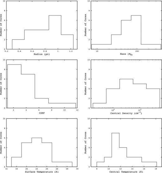
Histograms of (top row, left to right) core radius, core mass, (middle row) the ISRF surrounding the core and the core’s central density, and (lower row) the surface and central temperatures found in the cores. Note that the x axes for mass and central density use a logarithmic scale.

Open in new tabDownload slide

Rathborne et al. (2006) calculated the masses of 190 infrared dark cores and found a range between 10 and 2100 M_⊙, with a median of 120 M_⊙. However, they also found that 67 per cent of their cores have a mass between 30 and 300 M_⊙. By choosing only a few of the youngest, most nearby cores, we are more likely to pick only those with lower masses, so this discrepancy is most likely a selection effect. Fig. 4 shows the masses of our cores plotted against their radii and central densities. The masses of the cores do not appear to be correlated with either parameter.

Figure 4

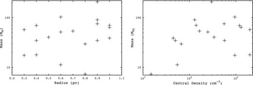
Core mass versus radius (left) and central density (right). No correlation is seen in either case.

Open in new tabDownload slide

4.2 Temperatures

When selecting our sources, the aim was to pick the youngest subset of infrared dark cores: those which show no internal MIR source and which were thus deemed to be starless. The lack of a MIR source makes it unlikely that these cores have any significant heating from within. The cores are, instead, heated by external radiation impinging on to their surfaces. This external heating results in a temperature gradient throughout each core, decreasing from surface to centre. Temperatures in individual cores have been observed to vary by up to 15 K (Peretto et al. 2010; Wilcock et al. 2011). It should be noted that the temperature profiles of the cores are not linear but rather show an exponential relationship with distance from the centre of the core. Two examples of temperature profiles are shown in Fig. 5.

Figure 5

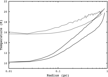
Temperature profiles of two typical cores. The solid line shows core 310.297+0.705 and the dashed line shows core 321.753+0.669. The top line of each pair shows a direction of θ= 0°, perpendicular to the mid-plane of the core, and the lower line shows θ= 90°, along the mid-plane of the core.

Open in new tabDownload slide

In Table 1, the temperatures at the centre of the core and at the surface are given. These have averages of 11 and 21 K, respectively. The dust temperatures in flattened cores show a variation at different directions within the cores. The cores are colder in their mid-planes (θ= 90°) than in the direction perpendicular to their mid-planes (θ= 0°). The outer layers of the cores show the biggest variation with direction. The surface temperatures show a greater range (varying by over 10 K) than the central temperatures (which have a range of less than 7 K). Fig. 3 shows the distribution of both sets of temperatures.

4.2.1 Surface temperatures

Fig. 6 shows the ISRF surrounding each core plotted against both the surface (upper panel; on a log scale) and central (lower panel) temperatures. The surface temperature is seen to be strongly dependent on the amount of radiation falling on the core. As a core’s major source of heating is from external radiation, this is as expected. The higher the local ISRF, the more radiation will fall on the core and the higher will be its surface temperature. The two show an exponential relationship, with increasing amounts of radiation needed to heat the core to greater temperatures.

Figure 6

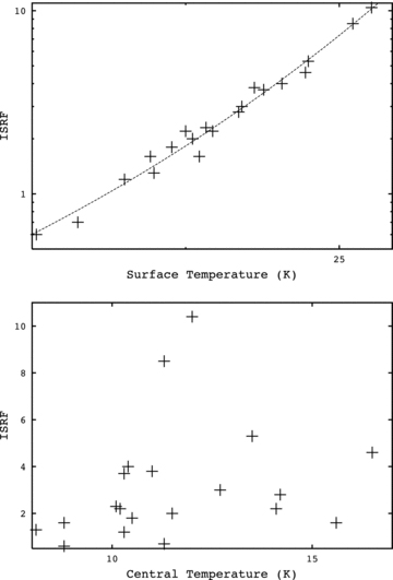
Upper: the ISRF in multiples of the Black (1994) radiation field plotted against the surface temperature. The dashed line shows the relation between the surface temperature and ISRF as described in equation (4). Lower: the ISRF in multiples of the Black (1994) radiation field plotted against the central temperature.

Open in new tabDownload slide

The correlation coefficient between the ISRF and T_s is r= 0.99, p < 0.05. r is the Pearson product moment correlation coefficient and p is the level of significance (i.e. p < 0.05 implies a 95 per cent confidence that a relationship exists).

The dotted line in Fig. 6 shows the best-fitting canonical relationship

4

where ISRF is the radiation field found in the vicinity of the core in multiples of the Black (1994) radiation field and T_s is the core’s surface temperature.

From equation (4), we extrapolate that for a core to have a surface temperature over 30 K the ISRF would need to be over 20 times that of the solar neighbourhood and for a surface temperature over 40 K the ISRF would have to be 100 times greater. Most infrared dark cores will therefore have a surface temperature lower than 30 K. The majority of our cores have surface temperatures less than 25 K.

Similarly, a core with a surface temperature less than 10 K would need to be situated in a radiation field of only one-hundredth of the solar value. This makes lower temperatures very unlikely, although not impossible. All of our cores had surface temperatures greater than 16 K.

4.2.2 Central temperatures

The temperatures at the centres of the cores vary according to different criteria to those at the surface. The central temperatures of the cores do not show any dependence on the ISRF – see the lower panel of Fig. 6. Instead, the temperature at the centre of the core appears to be determined by its mass and central density, as shown in Fig. 7.

Figure 7

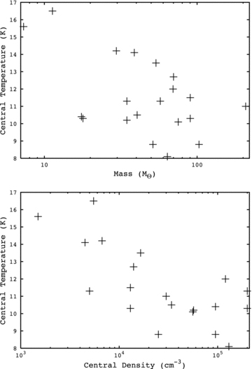
Upper: the mass of the cores plotted against their central temperatures. Lower: the central density of the cores plotted against their central temperatures.

Open in new tabDownload slide

The central temperature shows an inverse linear relationship with central density with a correlation coefficient of r=−0.46, p < 0.05. As radiation falls on to the core surface, it will heat the outer layers first, giving the temperature gradient visible in all IRDC cores. In denser cores, the radiation will have a greater probability of being absorbed in the outer layers and less will travel through the core to heat the centre. Thus, denser cores have a lower central temperature than cores with a lower density.

The masses of the cores show no relation to the temperature at the surface of the core but do show a weak anticorrelation with the central temperatures, r=−0.35, p < 0.05. Cores with high masses have a lower central temperature. This is due to the same effect that causes the central temperature to vary with density. As mentioned in Section 4.1, mass and central density show no correlation with one another. This implies that their relationships with central temperature must be independent of each other.

Fig. 8 shows the central temperature plotted against the surface temperature. The two show a broad correlation (r= 0.44, p < 0.05), implying that cores with a similar central density have a higher central temperature if there is a greater ISRF. However, the cores with highest surface temperatures do not necessarily have the highest central temperatures. For example, cores 307.495+0.660 and 326.811+0.656 have vastly different surface temperatures but identical central temperatures.

Figure 8

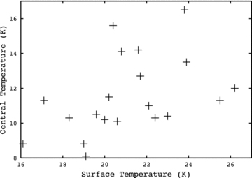
The temperature at the centre of the core versus the temperature at the surface of the core.

Open in new tabDownload slide

4.2.3 Temperature range

The range of temperatures in each core, ΔT, is found via

5

where T_c is the central temperature of the core and T_s is the surface temperature of the core. ΔT is indicative of a core’s temperature profile. A core with a high ΔT will show a steeper profile than a core with a lower ΔT. Fig. 5 shows the temperature profiles of two cores with similar radii. G310.297+0.705 has ΔT= 10.5 K and a far steeper profile than G321.753+0.669 which has ΔT= 4.8 K. ΔT appears to be dependent on a core’s central density (r= 0.81, p < 0.05) and the surrounding ISRF, but not with its mass (r= 0.27, p > 0.05). This is shown in Fig. 9. A possible exponential relation between ΔT and the ISRF can be seen. As this is similar to the relationship between ISRF and the surface temperature, it is likely a result of the ΔT dependence on surface temperature of the core.

Figure 9

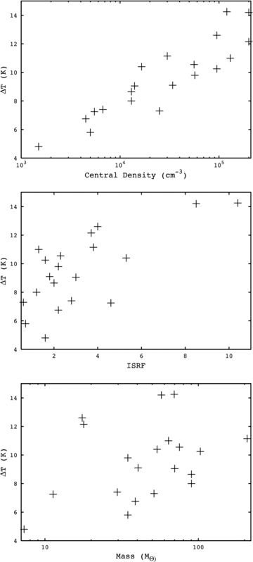
Upper: the central density of the cores plotted against the difference between the surface and central temperatures (ΔT). Middle: the ISRF in multiples of the Black (1994) radiation field plotted against ΔT. Lower: the masses of the cores plotted against ΔT.

Open in new tabDownload slide

The strongest relation is that between ΔT and the core’s central density. The difference between the temperature at the surface and centre of a core clearly increases as the central density increases. Radiation passing through denser material has a greater probability of being absorbed in the surface layers of the core, and so less radiation passes through to (and heats) the centre of the core. Therefore, if two cores are situated within areas of equivalent ISRFs then, while the surface temperatures would be the same, the denser core would have a colder centre and exhibit a wider range of temperature.

ΔT also shows a weak inverse correlation with the radius of a core (r=−0.55, p < 0.05) – see Fig. 10. The larger the size of the core, the smaller the temperature difference between the surface and the centre. This is the opposite of what one would generally expect and, as it is a weak relationship, is not likely to be a direct result but rather a side effect of the fact that our smallest cores have the highest densities.

Figure 10

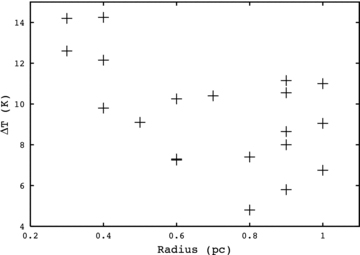
ΔT versus radius.

Open in new tabDownload slide

4.3 Central densities

The central densities of the cores vary from 1.5 × 10³ to 2.0 × 10⁵ cm⁻³, with a mean of 2.0 × 10⁴ cm⁻³. The central density of the core is an input to the phaethon code and mostly affects the longer wavelength end of the SED. Fig. 3 shows the distribution of central densities. The density profile of each core is calculated via equation (3). This results in the density at the surface of the core (where it is at its lowest) directly correlating with the maximum central density. It is simply an input definition of the model. The surface densities range from 0.1 to 20 cm⁻³.

Fig. 11 shows the central density of each core plotted against its radius. There is no obvious correlation between the two but there is a notable lack of cores in the lower left-hand corner with both a low central density and a small radius. This is likely to be a selection effect. This implies that either small, low density cores do not show up as a distinct peak against their parent cloud, or they do not block enough MIR background emission to show a significant dip at 8 m, or that they are simply fainter and so are more likely to be confused at 500 m.

Figure 11

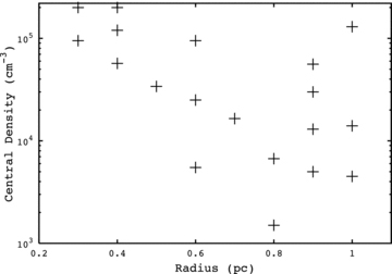
Central density versus radius.

Open in new tabDownload slide

This latter theory was tested by creating two model cores that would reside in the lower-left of Fig. 11. Both had a radius of 0.3 pc, equal to the smallest core we model. One had a central density of 2 × 10³ cm⁻³ and the other had 2 × 10⁴ cm⁻³. We placed both of them at a distance of 3.1 kpc, gave them an ISRF of 3.2 times the Black (1994) radiation field and an asymmetry factor of 2.5 (these are the average parameters of our modelled cores). The resulting objects have masses of 0.4 and 3.9 M_⊙. The cores were added to the Hi-GAL data in several regions and studied as with the original PF09 cores. Even in very low background regions, neither core met our criteria for isolation at 500 m. They would not have been selected by our observations.

4.4 The interstellar radiation field

The ISRF for each core is quoted in terms of multiples of the Black (1994) radiation field. The Black (1994) radiation field models the ISRF in the solar neighbourhood and measures a value of 1.3 × 10⁻¹⁶ erg s⁻¹ cm⁻² Hz⁻¹ sr⁻¹ at 500 m. Along with the central density, the ISRF is one of the inputs of the phaethon code (see Section 3.3), and mostly affects the SED at shorter wavelengths. The ISRF around our cores ranges from 0.6 to 10.4 times the Black (1994) field, with an average multiple of 3.2. Fig. 3 shows the distribution of the cores’ ISRF.

The amount of radiation incident on our cores is typically greater than that which we observe in the solar neighbourhood. This is consistent with the inner Galactic plane generally having a stronger radiation field than that of the solar neighbourhood. However, two of the cores do show a radiation field lower than the solar value. These are 307.495+0.660 and 321.678+0.965 (see Table 1). There are two possible explanations for this: either they simply exist in an area which has a particularly low ISRF or the ISRF surrounding the parent IRDC is consistent with other cores but the parent cloud is absorbing most of the radiation. The latter could be caused by the IRDC being especially dense, or by the cores being more deeply embedded within the parent cloud. Either case would make it difficult for radiation to penetrate far enough to affect the cores.

Fig. 12 shows a plot of core radius versus ISRF. We detect cores of all sizes with ISRFs at the lower end of our scale but our modelled sample does not include any cores with a high ISRF and a large radius. If radiation pressure were forcing the cores to condense, then we would expect the central density to increase as the radius decreased. While our smaller cores do tend to have densities at the higher end of our range, the larger cores have both low and high densities. This is due to the selection effect discussed in Section 4.3. We therefore dismiss radiation pressure as the reason why we detect no large cores in areas of high ISRF. Instead, we consider that in areas with a high radiation field, the outer layers of large cores may ‘boil away’ due to the large amounts of energy being absorbed. This would explain why we only see small cores in areas of high ISRF and why there is no significant increase in the density of these cores.

Figure 12

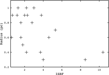
Core radius versus ISRF – in multiples of the Black (1994) radiation field.

Open in new tabDownload slide

The radius and surface temperature appear to show a similar, albeit inverse, relationship to that of ISRF and radius. We speculate that the radius of a core is actually affected by the ISRF and that any correlation between temperature and radius exists as a result of the dependence of the surface temperature on the ISRF.

4.5 Asymmetry factor

The asymmetry factor input to the model controls the shape of the core. A value of 1.0 would result in a circular core. The ellipticity of the core is increased by raising the asymmetry factor up to a maximum of 3.0. Most IRDC cores are elongated and have a high eccentricity. 80 per cent of our cores have an asymmetry factor greater than 2 – see Table 1. It is also possible that some of our more circular cores could be elongated but viewed end-on.

4.6 Mean core properties

Table 4 shows the mean values of each of the eight physical properties discussed in Sections 4.1–4.5. The mean physical properties reiterate the fact that starless cores are dense elongated cold objects and, when found in the Galactic plane, have a local ISRF greater than that found in the solar neighbourhood. Within the cores, the temperature decreases from surface to centre, typically by ∼10 K. The mean asymmetry factor is 2.5, corresponding to an aspect ratio of ∼1:7.

5 SUMMARY

Using data from the Herschel and Spitzer, 20 isolated starless cores were modelled with the phaethon radiative transfer code. A flattened density profile, as described by equation (3), was assumed for all. The FWHM of each core was measured at 250 m and used as the core’s radius. The radial distance for which the central density is constant was set to one-tenth of this value. The density and surrounding ISRF were varied until the model SED matched the observed SED at 160, 250, 350 and 500 m.

Output parameters were measured from the model. The IRDC cores were found to have masses ranging from around ten to around a few hundred solar masses. The masses of the cores were found not to correlate with their size or central density. The temperature at the surface of a core was seen to depend almost entirely on the level of the ISRF surrounding the core. No correlation was found between the temperature at the centre of a core and its local ISRF. The central temperature was seen to depend, instead, on the density and mass of the core. A core with a high density or mass is likely to have a lower central temperature.

The range of temperatures from centre to edge in any one core was found to correlate strongly with the central density of that core. Low density cores exhibit a much smaller range of temperatures and thus a shallower temperature gradient than higher density cores. The cores situated in a high ISRF (and thus with a high surface temperature) are also likely to show a greater range of temperature from centre to edge.

No large cores were found within an area of comparatively high ISRF. However, there appears to be no correlation between the ISRF surrounding a core and its central density. Hence, we rule out radiation pressure as the cause. Instead, we consider that the outer layers of cores in areas of high radiation may be evaporated due to the high levels of energy being absorbed, leaving only smaller cores in high-ISRF regions. 16 out of 20 isolated IRDC cores showed high levels of ellipticity.

LAW gratefully acknowledges STFC studentship funding. SPIRE was developed by a consortium of institutes led by Cardiff University (UK) and including University Lethbridge (Canada); NAOC (China); CEA, LAM (France); IFSI, University Padua (Italy); IAC (Spain); Stockholm Observatory (Sweden); Imperial College London, RAL, UCL-MSSL, UKATC, University Sussex (UK) and Caltech, JPL, NHSC, University Colorado (USA). This development has been supported by national funding agencies: CSA (Canada); NAOC (China); CEA, CNES, CNRS (France); ASI (Italy); MCINN (Spain); SNSB (Sweden); STFC (UK) and NASA (USA). PACS was developed by a consortium of institutes led by MPE (Germany) and including UVIE (Austria); KU Leuven, CSL, IMEC (Belgium); CEA, LAM (France); MPIA (Germany); INAF-IFSI/OAA/OAP/OAT, LENS, SISSA (Italy) and IAC (Spain). This development has been supported by the funding agencies BMVIT (Austria), ESA-PRODEX (Belgium), CEA/CNES (France), DLR (Germany), ASI/INAF (Italy) and CICYT/MCYT (Spain). HIPE is a joint development by the Herschel Science Ground Segment Consortium, consisting of ESA, the NASA Herschel Science Center, and the HIFI, PACS and SPIRE consortia.

Footnotes

REFERENCES

Appendix

APPENDIX A: Examples of the modelled cores

Fig. A1 is a sample of the full appendix, which is available as Supporting Information with the online version of the article.

Figure A1

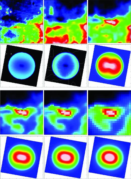
305.798−0.097 – Upper row: observational images of the infrared dark core at (left–right) Spitzer 8 m, PACS 70 m and PACS 160 m. Second row: modelled images at 8, 70 and 160 m. Third row: observational at SPIRE 250, 350 and 500 m. Lower row: modelled images at 250, 350 and 500 m. All images are ∼0.05°× 0.05° in size, equivalent to 2.56 pc × 2.56 pc.

Open in new tabDownload slide

SUPPORTING INFORMATION

Additional Supporting Information may be found in the on-line version of this article:

Appendix A. Examples of the modelled cores.

Please note: Wiley-Blackwell are not responsible for the content or functionality of any supporting materials supplied by the authors. Any queries (other than missing material) should be directed to the corresponding author for the article.