Image analysis for cosmology: results from the GREAT10 Galaxy Challenge Free

Abstract

1 INTRODUCTION

In this paper, we present the results from the GRavitational lEnsing Accuracy Testing 2010 (GREAT10) Galaxy Challenge. GREAT10 was an image analysis challenge for cosmology that focused on the task of measuring the weak-lensing signal from galaxies. Weak lensing is the effect whereby the image of a source galaxy is distorted by intervening massive structure along the line of sight. In the weak field limit, this distortion is a change in the observed ellipticity of the object, and this change in ellipticity is called shear. Weak lensing is particularly important for understanding the nature of dark energy and dark matter, because it can be used to measure the cosmic growth of structure and the expansion history of the Universe (see reviews by e.g. Albrecht et al. 2006; Bartelmann & Schneider 2001; Hoekstra & Jain 2008; Massey, Kitching & Richards 2010; Weinberg et al. 2012). In general, by measuring the ellipticities of distant galaxies – hereafter denoted by ‘shape measurement’– we can make statistical statements about the nature of the intervening matter. The full process through which photons propagate from galaxies to detectors is described in a previous companion paper, the GREAT10 Handbook (Kitching et al. 2011).

There are a number of features, in the physical processes and optical systems, through which the photons we ultimately use for weak lensing pass. These features must be accounted for when designing shape measurement algorithms. These are primarily the convolution effects of the atmosphere and the telescope optics, pixelization effects of the detectors used and the presence of noise in the images. The simulations in GREAT10 aimed to address each of these complicating factors. GREAT10 consisted of two concurrent challenges as described in Kitching et al. (2011): the Galaxy Challenge, where entrants were provided with 50 million simulated galaxies and asked to measure their shapes and spatial variation of the shear field with a known point spread function (PSF) and the Star Challenge wherein entrants were provided with an unknown PSF, sampled by stars, and asked to reconstruct the spatial variation of the PSF across the field.

In this paper, we present the results of the GREAT10 Galaxy Challenge. The challenge provided a controlled simulation development environment in which shape measurement methods could be tested, and was run as a blind competition for 9 months from 2010 December to 2011 September. Blind analysis of shape measurement algorithms began with the Shear TEsting Programme (STEP; Heymans et al. 2006; Massey et al. 2007) and GREAT08 (Bridle et al. 2009, 2010). The blindness of these competitions is critical in testing methods under circumstances that will be similar to those encountered in real astronomical data. This is because for weak lensing, unlike photometric redshifts, for example, we cannot observe a training set from which we know the shear distribution. [We can, however, observe a subset of galaxies at high signal-to-noise ratio (S/N) to train upon, which is something we address in this paper.]

The GREAT10 Galaxy Challenge is the first shape measurement analysis that includes variable fields. Both the shear field and the PSF vary across the images in a realistic manner. This enables a variety of metrics that are inaccessible to constant shear simulations (where the fields are a single constant value across the images), including a direct measure of the impact of shape measurement inaccuracies on the inferred shear power spectrum and a measure of the correlations among shape measurement inaccuracies and the size and ellipticity of the PSF.

We present a general pseudo-C_ℓ formalism for a flat-sky shear field in Appendix A, which we use to show how to propagate general spatially varying shear measurement biases through to the shear power spectrum. This has a more general application in cosmic shear studies.

This paper summarizes the results of the GREAT10 Galaxy Challenge. We refer the reader to a companion paper that discusses the GREAT10 Star challenge (Kitching et al., in preparation). Here we summarize the results that we show, distilled from the wealth of information that we present in this paper:

• Signal-to-noise ratio. We find a strong dependence of the metrics below S/N= 10. However, we find methods that meet bias requirements for the most ambitious experiments when S/N > 20. We note that methods tested here have been optimized for use on ground-based data in this regime.

• Galaxy type. We find marginal evidence that model-fitting methods have a relatively low dependence on galaxy type compared to model-independent methods.

• PSF dependence. We find contributions to biases from PSF size, but less so from PSF ellipticity.

• Galaxy size. For large galaxies well sampled by the PSF, with scale radii ≳2 times the mean PSF size, we find that methods meet requirements on bias parameters for the most ambitious experiments. However, if galaxies are unresolved, with radii ≲1 time the mean PSF size, biases become significant.

• Training. We find that calibration on a high-S/N sample can significantly improve a method’s average biases.

• Averaging methods. We find that averaging ellipticities over several methods is clearly beneficial, but that the weight assigned to each method will need to be correctly determined.

In Section 2, we describe the Galaxy Challenge structure and in Section 3 we describe the simulations. Results are summarized in Section 4 and we present conclusions in Sections 5 and 6. We make extensive use of appendices that contain technical information on the metrics and a more detailed breakdown of individual shape measurement methods’ performance.

2 DESCRIPTION OF THE COMPETITION

The GREAT10 Galaxy Challenge was run as an open competition for 9 months between 2010 December 3 and 2011 September 2.1 The challenge was open for participation from anyone, the website2 served as the portal for participants, and data could be freely downloaded.

The challenge was to reconstruct the shear power spectrum from subsampled images of sheared galaxies (Kitching et al. 2011). All shape measurement methods to date do this by measuring the ellipticity from each galaxy in an image, although scope for alternative approaches was allowed. Participants in the challenge were asked to submit either

• Ellipticity catalogues that contained an estimate of the ellipticity for each object in each image; or

• Shear power spectra that consisted of an estimate of the shear power spectrum for each simulation set.

For ellipticity catalogue submissions, all objects were required to have an ellipticity estimate, and no galaxies were removed or downweighted in the power spectrum calculation; if such weighting functions were desired by a participant, then a shear power spectrum submission was encouraged.

Participants were required to access 1 TB of imaging data in the form of FITS images. Each image contained 10 000 galaxies arranged on a 100 × 100 grid. Each galaxy was captured in a single postage stamp of 48 × 48 pixels (to incorporate the largest galaxies in the simulation with no truncation), and the grid was arranged so that each neighbouring postage stamp was positioned contiguously, that is, there were no gaps between postage stamps and no overlaps. Therefore, each image was 4800 × 4800 pixels in size. The simulations were divided into 24 sets (see Section 3.1) and each set contained 200 images. For each galaxy in each image, participants were provided with a functional description of the PSF (described in Appendix C3) and an image showing a pixelized realization of the PSF. In addition, a suite of development code were provided to help read in the data and perform a simple analysis.3

2.1 Summary of metrics

The metric with which the live leaderboard was scored during the challenge was a quality factor Q, defined as

1

averaged over all sets, a quantity that relates the reconstructed shear power spectrum with the true shear power spectrum ⁠. We describe this metric in more detail in Appendices A and B. This is a general integral expression for the quality factor; in the simulations, we use discrete bins in ℓ which are defined in Appendix C. By evaluating this metric for each submission, results were posted to a live leaderboard that ranked methods based on the value of Q. We will also investigate a variety of alternative metrics extending the STEP m and c bias formalism to variable fields.

The measured ellipticity of an object at position can be related to the true ellipticity and shear,

2

with a multiplicative bias ⁠, an offset ⁠, and a quadratic term (this is γ|γ|, not γ², since we may expect divergent behaviour to more positive and more negative shear values for each domain, respectively), which in general are functions of position due to PSF and galaxy properties. is a potential stochastic noise contribution. For spatially variable shear fields, biases between measured and true shear can vary as a function of position, mixing angular modes and power between E and B modes. In Appendix A, we present a general formalism that allows for the propagation of biases into shear power spectra using a pseudo-C_ℓ methodology; this approach has applications beyond the treatment of shear systematics. The full set of metrics are described in detail in Appendix B and are summarized in Table 1.

Table 1

Open in new tab

A summary of the metrics used to evaluate shape measurement methods for GREAT10. These are given in detail in Appendices A and B. We refer to m and c as the one-point estimators of bias, and make the distinction between these and spatially constant terms (m₀, c₀) and correlations (α, β) only where clearly stated.

Metric	Definition	Features
m, c, q		One-point estimators of bias. Links to STEP
Q		Numerator relates to bias on w0
Qdn		Corrects Q for pixel noise
⁠,		Power spectrum relations
αX		Variation of m with PSF ellipticity/size
βX		Variation of c with PSF ellipticity/size

Metric	Definition	Features
m, c, q		One-point estimators of bias. Links to STEP
Q		Numerator relates to bias on w0
Qdn		Corrects Q for pixel noise
⁠,		Power spectrum relations
αX		Variation of m with PSF ellipticity/size
βX		Variation of c with PSF ellipticity/size

Table 1

Open in new tab

A summary of the metrics used to evaluate shape measurement methods for GREAT10. These are given in detail in Appendices A and B. We refer to m and c as the one-point estimators of bias, and make the distinction between these and spatially constant terms (m₀, c₀) and correlations (α, β) only where clearly stated.

Metric	Definition	Features
m, c, q		One-point estimators of bias. Links to STEP
Q		Numerator relates to bias on w0
Qdn		Corrects Q for pixel noise
⁠,		Power spectrum relations
αX		Variation of m with PSF ellipticity/size
βX		Variation of c with PSF ellipticity/size

Metric	Definition	Features
m, c, q		One-point estimators of bias. Links to STEP
Q		Numerator relates to bias on w0
Qdn		Corrects Q for pixel noise
⁠,		Power spectrum relations
αX		Variation of m with PSF ellipticity/size
βX		Variation of c with PSF ellipticity/size

The metric with which the live leaderboard was scored was the Q value, and the same metric was used for ellipticity catalogue submissions and power spectrum submissions. However, in this paper, we will introduce and focus on Q_dn (see Table 1) which for ellipticity catalogue submissions removes any residual pixel-noise error (nominally associated with biases caused by finite S/N or inherent shape measurement method noise). For details, see Appendix B. Note that this is not a correction for ellipticity (shape) noise which is removed in GREAT10 through the implementation of a B-mode-only intrinsic ellipticity field.

The metric Q takes into account scatter between the estimated shear and the true shear due to stochasticity in a method or spatially varying quantities, such that a small and do not necessarily correspond to a large Q value (see Appendix B). This is discussed within the context of previous challenges in Kitching et al. (2008). Spatial variation is important because the shear and PSF fields vary, so that there may be scale-dependent correlations between them, and stochasticity is important because we wish methods to be accurate (such that errors do not dilute cosmological or astrophysical constraints) as well as being unbiased.

For variable fields, we can complement the linear biases, and ⁠, with a component that can be correlated with any spatially varying quantity ⁠, for example, PSF ellipticity or size:

3

with spatially constant terms m₀ and c₀ and correlation coefficients α and β; X₀ is a constant reference value that ensures that the units of α and β are dimensionless: for ellipticity this is set to unity, X₀= 1, and for PSF size squared, this is the mean PSF size squared, ⁠. Only ellipticity catalogue submissions can have m₀, c₀, α and β values calculated because these parameters require individual galaxy ellipticity estimates (in order to calculate the required mixing matrices, see Appendices A and B). Throughout we will refer to m and c as the one-point estimators of bias and make the distinction between spatially constant terms m₀ and c₀ and correlations α and β only where clearly stated. Finally, we also include a non-linear shear response (see Table 1); we do not include a discussion of this in the main results, because qγ|γ| ≈ 0 for most methods, but show the results in Appendix E.

To measure biases at the power spectrum level, we define constant linear bias parameters (see Appendix A, equation A13),

4

which relate the measured power spectrum to the true power spectrum. These are approximately related to one-point shear bias m, and the variance of c, by for values of m≪ 1 and ⁠. These parameters can be calculated for both ellipticity and power spectrum submissions.

3 DESCRIPTION OF THE SIMULATIONS

In this section, we describe the overall structure of the simulations. For details on the local modelling of the galaxy and star profiles and the spatial variation of the PSF and shear fields, we refer the reader to Appendix C.

3.1 Simulation structure

The structure of the simulations was engineered such that, in the final analysis, the various aspects of performance for a given shape measurement method could be gauged. The competition was split into sets of images, where one set was a ‘fiducial’ set and the remaining sets represented perturbations about the parameters in that set. Each set consisted of 200 images. This number was justified by calculating the expected pixel-noise effect on shape measurement methods (see Appendix B) such that when averaging over all 200 images this effect should be suppressed (however, see also Section 4 where we investigate this noise term further).

Participants were provided with a functional description and a pixelated realization of the PSF at each galaxy position. The task of estimating the PSF itself was set a separate ‘Star Challenge’ which is described in a companion paper (Kitching et al., in preparation).

The variable shear field was constant in each of the images within a set, but the PSF field and intrinsic ellipticity could vary such that there were three kinds of sets:

• Type 1. ‘Single epoch’, fixed ⁠, variable PSF, variable intrinsic ellipticity.

• Type 2. ‘Multi-epoch’, fixed ⁠, variable PSF, fixed intrinsic ellipticity.

• Type 3. ‘Stable single epoch’, fixed ⁠, fixed PSF, variable intrinsic ellipticity.

The default, fiducial, type being one in which both PSF and intrinsic ellipticity vary between images in a set. This was designed in part to test the ability of any method that took advantage of stacking procedures, where galaxy images are averaged over some population, by testing whether stacking worked when either the galaxy or the PSF was fixed across images within a set. Stacking methods achieved high scores in GREAT08 (Bridle et al. 2010), but in actuality were not submitted for GREAT10. For each type of set, the PSF and intrinsic ellipticity fields are always spatially varying, but this variation did not change within a set; when we refer to a quantity being ‘fixed’, it means that its spatial variation does not vary between images within a set.

Type 1 (variable PSF and intrinsic field) sets test the ability of a method to reconstruct the shear field in the presence of both a variable PSF field and variable intrinsic ellipticity between images. This nominally represents a sequence of observations of different patches of sky but with the same underlying shear power spectrum. Type 2 sets (variable PSF and fixed intrinsic field) represent an observing strategy where the PSF is different in each exposure of the same patch of sky (a typical ground-based observation), the so-called ‘multi-epoch’ data. Type 3 sets (fixed PSF) represent ‘single-epoch’ observations with a highly stable PSF. These were only simple approximations to reality, because, for example, properties in the individual exposures for the ‘multi-epoch’ sets were not correlated (as they may be in real data), and the S/N was constant in all images for the single and multi-epoch sets. Participants were aware of the PSF variation from image to image within a set but not of the intrinsic galaxy properties or shear. Thus, the conclusions drawn from these tests will be conservative with regard to the testing between the different set types, relative to real data, where in fact this kind of observation is known to the observer ab initio. In subsequent challenges, this hidden layer of complexity could be removed.

In Appendix D, we list in detail the parameter values that define each set, and the parameters themselves are described in the sections below. In Table 2, we summarize each set by listing its distinguishing feature and parameter value.

There were two additional sets that used a pseudo-Airy PSF which we do not include in this paper because of technical reasons (see Appendix F).

Training data were provided in the form of a set with exactly the same size and form as the other sets. In fact the training set was a copy of Set 7, a set which contained high-S/N galaxies. In this way, the structure was set up to enable an assessment of whether training on high-S/N data is useful when extrapolating to other domains, in particular low-galaxy-S/N regime. This is similar to being able to observe a region of sky with deeper exposures than a main survey.

3.2 Variable shear and intrinsic ellipticity fields

In the GREAT10 simulations, the key and unique aspect was that the shear field was a variable quantity and not a static scalar value (as for all previous shape measurement simulations; STEP1, STEP2, GREAT08). To make a variable shear field, we generated a spin-2 Gaussian random field from a Λ cold dark matter weak-lensing power spectrum (Hu 1999):

5

where P_δδ is the matter power spectrum, and the lensing weight can be expressed as

6

where the kernel is

7

We have assumed a flat Euclidean geometry throughout and r_H is the horizon size. p_i(r) refers to the redshift distribution of the lensed sources in redshift bin i; this expression can be generalized to an arbitrary number (even a continuous set) of redshift bins (see Kitching, Heavens & Miller 2011). For these simulations, we have a single redshift bin with a median redshift of z_m= 1.0 and a delta function probability distribution p_i(r′) =δ^D(r−r_i). We assume an Eisenstein & Hu (1999) linear matter power spectrum with a Smith et al. (2003) non-linear correction. The cosmological parameter values used were Ω_m= 0.25, h=H₀/100 = 0.75, n_s= 0.95 and σ₈= 0.78. In order to add a random component to the shear power spectrum, so that participants could not guess the functional form, we added a series of Legendre polynomials P_n(x) up to fifth order, such that

8

where the variable x_L=−1 + 2(ℓ− 1)/(ℓ_max− 1) is contained within the range [−1, 1] as ℓ varies from ℓ_min to ℓ_max. The shear field generated has an E-mode power spectrum only. The size of the shear field was and to generate the shear field we set θ_image= 10°, such that the range in ℓ we used to generate the power was ℓ= [36, 3600] from the fundamental mode to the grid separation cut-off; the exact ℓ modes used are given in Appendix C. Note that the Legendre polynomials add fluctuations to the power spectra; this is benign in the calculation of the evaluation metrics but would not be expected from real data.

The shear field is generated on a grid of 100 × 100 pixels, which is then converted into an image of galaxy objects via an image generation code4 with galaxy properties described in Appendix C. When postage stamps of objects are generated, they point-sample the shear field at each position, and a postage stamp is generated. The postage stamps are then combined to form an image.

Throughout, the intrinsic ellipticity field had a variation that contained B-mode power only (in every image and when also averaged over all images in a set), as described in the GREAT10 Handbook. This meant that the contribution from intrinsic ellipticity correlations, as well as from intrinsic shape noise, to the lensing shear power spectra was zero.

4 RESULTS

In total, the challenge received 95 submissions from nine separate teams and 12 different methods. These were as follows:

• 82 submissions before the deadline

• 13 submissions in the post-challenge period

which were split into

• 85 ellipticity catalogue submissions

• 10 power spectrum submissions

We summarize the methods that analysed the GREAT10 Galaxy Challenge in detail in Appendix E. The method that won the challenge, with the highest Q value at the end of the challenge period, was ‘fit2-unfold’ submitted by the DeepZot team (formed by authors DK and DM).

During the challenge a number of aspects of the simulations were corrected (we list these in Appendix F). Several methods generated low scores due to misunderstanding of simulation details, and in this paper we summarize only those results for which these errata did not occur. In the following, we choose the best performing entry for each of the 12 shape measurement method entries.

4.1 One-point estimators of bias: m and c values

In Appendix B, we describe how the estimators for shear biases on a galaxy-by-galaxy basis in the simulations – what we refer to as ‘one-point estimators’ of biases – can be derived, and how these relate to the STEP m and c parameters (Heymans et al. 2006). In Fig. 1 and Table 3, we show the m and c biases for the best performing entries for each method (those with the highest quality factors). In Appendix E, we show how the m and c parameters, and the difference between the measured and true shear, ⁠, vary for each method as a function of several quantities: PSF ellipticity, PSF size, galaxy size, galaxy bulge-to-disc ratio and galaxy bulge-to-disc angle offset. We show in Appendix E that some methods have a strong m dependence on PSF ellipticity and size [e.g. Total Variation Neural Network (TVNN) and method04]. Model-fitting methods (gfit, im3shape) tend to have fewer model-dependent biases, whereas the KSB-like methods (DEIMOS, KSB f90) have the smallest average biases.

Figure 1

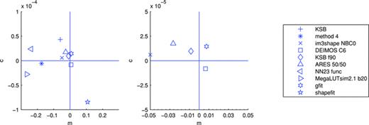
In the left-hand panel, we show the multiplicative m and additive c biases for each ellipticity catalogue method, for which one-point estimators can be calculated (see Appendix B). The symbols indicate the methods with a legend in the right-hand panel. The central panel expands the x- and y-axes to show the best performing methods.

Open in new tabDownload slide

Table 3

Open in new tab

The quality factors, Q, with denoising and training, and the m and c values for each method (not available for power spectrum submissions) that we explore in detail in this paper, in alphabetical order of the method name. A ‘(ps)’ indicates a power spectrum submission; in these cases, Q_{dn & trained}=Q_trained; all others were ellipticity catalogue submissions. An * indicates that this team had knowledge of the internal parameters of the simulations, and access to the image simulation code. A † indicates that this submission was made in the post-challenge time period.

Method	Q	Qdn	Qdn & trained	m	c/10−4
†ARES 50/50	105.80	163.44	277.01	−0.026 483	0.35	−0.018 566	0.0728
†cat7unfold2 (ps)	152.55		150.37			0.021 409	0.0707
DEIMOS C6	56.69	103.87	203.47	0.006 554	0.08	0.004 320	0.6329
fit2-unfold (ps)	229.99		240.11			0.040 767	0.0656
gfit	50.11	122.74	249.88	0.007 611	0.29	0.005 829	0.0573
*im3shape NBC0	82.33	114.25	167.53	−0.049 982	0.12	−0.053 837	0.0945
KSB	97.22	134.42	166.96	−0.059 520	0.86	−0.037 636	0.0872
*KSB f90	49.12	102.29	202.83	−0.008 352	0.19	0.020 803	0.0789
†MegaLUTsim2.1 b20	69.17	75.30	52.62	−0.265 354	−0.55	−0.183 078	0.1311
method04	83.52	92.66	116.02	−0.174 896	−0.12	−0.090 748	0.0969
†NN23 func	83.16	60.92	17.19	−0.239 057	0.47	−0.015 292	0.0982
shapefit	39.09	63.49	84.68	0.108 292	0.17	0.049 069	0.8686

Method	Q	Qdn	Qdn & trained	m	c/10−4
†ARES 50/50	105.80	163.44	277.01	−0.026 483	0.35	−0.018 566	0.0728
†cat7unfold2 (ps)	152.55		150.37			0.021 409	0.0707
DEIMOS C6	56.69	103.87	203.47	0.006 554	0.08	0.004 320	0.6329
fit2-unfold (ps)	229.99		240.11			0.040 767	0.0656
gfit	50.11	122.74	249.88	0.007 611	0.29	0.005 829	0.0573
*im3shape NBC0	82.33	114.25	167.53	−0.049 982	0.12	−0.053 837	0.0945
KSB	97.22	134.42	166.96	−0.059 520	0.86	−0.037 636	0.0872
*KSB f90	49.12	102.29	202.83	−0.008 352	0.19	0.020 803	0.0789
†MegaLUTsim2.1 b20	69.17	75.30	52.62	−0.265 354	−0.55	−0.183 078	0.1311
method04	83.52	92.66	116.02	−0.174 896	−0.12	−0.090 748	0.0969
†NN23 func	83.16	60.92	17.19	−0.239 057	0.47	−0.015 292	0.0982
shapefit	39.09	63.49	84.68	0.108 292	0.17	0.049 069	0.8686

Table 3

Open in new tab

The quality factors, Q, with denoising and training, and the m and c values for each method (not available for power spectrum submissions) that we explore in detail in this paper, in alphabetical order of the method name. A ‘(ps)’ indicates a power spectrum submission; in these cases, Q_{dn & trained}=Q_trained; all others were ellipticity catalogue submissions. An * indicates that this team had knowledge of the internal parameters of the simulations, and access to the image simulation code. A † indicates that this submission was made in the post-challenge time period.

Method	Q	Qdn	Qdn & trained	m	c/10−4
†ARES 50/50	105.80	163.44	277.01	−0.026 483	0.35	−0.018 566	0.0728
†cat7unfold2 (ps)	152.55		150.37			0.021 409	0.0707
DEIMOS C6	56.69	103.87	203.47	0.006 554	0.08	0.004 320	0.6329
fit2-unfold (ps)	229.99		240.11			0.040 767	0.0656
gfit	50.11	122.74	249.88	0.007 611	0.29	0.005 829	0.0573
*im3shape NBC0	82.33	114.25	167.53	−0.049 982	0.12	−0.053 837	0.0945
KSB	97.22	134.42	166.96	−0.059 520	0.86	−0.037 636	0.0872
*KSB f90	49.12	102.29	202.83	−0.008 352	0.19	0.020 803	0.0789
†MegaLUTsim2.1 b20	69.17	75.30	52.62	−0.265 354	−0.55	−0.183 078	0.1311
method04	83.52	92.66	116.02	−0.174 896	−0.12	−0.090 748	0.0969
†NN23 func	83.16	60.92	17.19	−0.239 057	0.47	−0.015 292	0.0982
shapefit	39.09	63.49	84.68	0.108 292	0.17	0.049 069	0.8686

Method	Q	Qdn	Qdn & trained	m	c/10−4
†ARES 50/50	105.80	163.44	277.01	−0.026 483	0.35	−0.018 566	0.0728
†cat7unfold2 (ps)	152.55		150.37			0.021 409	0.0707
DEIMOS C6	56.69	103.87	203.47	0.006 554	0.08	0.004 320	0.6329
fit2-unfold (ps)	229.99		240.11			0.040 767	0.0656
gfit	50.11	122.74	249.88	0.007 611	0.29	0.005 829	0.0573
*im3shape NBC0	82.33	114.25	167.53	−0.049 982	0.12	−0.053 837	0.0945
KSB	97.22	134.42	166.96	−0.059 520	0.86	−0.037 636	0.0872
*KSB f90	49.12	102.29	202.83	−0.008 352	0.19	0.020 803	0.0789
†MegaLUTsim2.1 b20	69.17	75.30	52.62	−0.265 354	−0.55	−0.183 078	0.1311
method04	83.52	92.66	116.02	−0.174 896	−0.12	−0.090 748	0.0969
†NN23 func	83.16	60.92	17.19	−0.239 057	0.47	−0.015 292	0.0982
shapefit	39.09	63.49	84.68	0.108 292	0.17	0.049 069	0.8686

4.2 Variable shear

In the left-hand panel of Fig. 2, we show the values of the linear power spectrum parameters and for each method for each set, and display by colour code the quality factor Q_dn. In Table 3, we show the mean values of these parameters averaged over all sets. We find a clear anticorrelation among ⁠, and Q_dn, with higher quality factors corresponding to smaller and values. We will explore this further in the subsequent sections. We refer the reader to Appendix B where we show how the ⁠, and Q_dn parameters are expected to be related in an ideal case. In the right-hand panel of Fig. 2, we also show the ⁠, and Q_dn values for each method averaged over all sets.

Figure 2

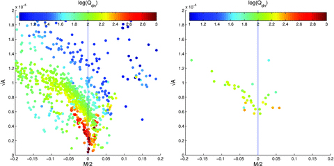
In the left-hand panel, we show and for each method for each set. The colour scale represents the logarithm of the quality factor Q_dn. In the right-hand panel, we show the metrics ⁠, and Q_dn for each method averaged over all sets. For a breakdown of these into dependence on set type, see Fig. 4.

Open in new tabDownload slide

In the left-hand panel of Fig. 3, we show the effect that the pixel noise denoising step has on the quality factor Q. Note that the way in which the denoising step is implemented here uses the variance of the true shear values (but not the true shear values themselves). This is a method which was not available to power spectrum submissions and indeed part of the challenge was to find optimal ways to account for this in power spectrum submissions. The final layer used to generate the ‘fit2-unfold’ submission performed power spectrum estimation and used the model-fitting errors themselves to determine and subtract the variance due to shape measurement errors, including pixel noise. We find as expected that Q in general increases for all methods when pixel noise is removed, by a factor of ≲1.5, such that a method that has Q≃ 100 has Q_dn≃ 150. When this correction is applied, the method ‘fit2-unfold’ still obtains the highest quality factor, and the ranking of the top five methods is unaffected.

Figure 3

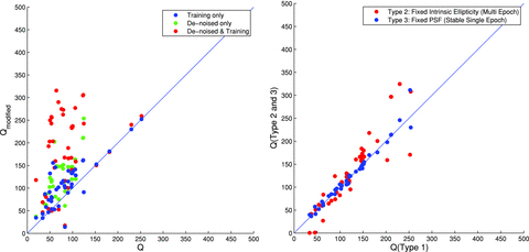
In the left-hand panel, we show the unmodified quality factor Q (equation 1) and how this relates to the quality factor with pixel (shape measurement) noise removed Q_dn and the quality factor obtained when high-S/N training is applied to each submission (equation 9). Methods that submitted power spectra could not be modified to remove the denoising in this way, so only the training values are shown. The right-hand panel shows the Q_dn for those sets with fixed intrinsic ellipticities (‘multi-epoch’; Type 2) or a fixed PSF (‘stable single epoch’; Type 3) over all images compared to the quality factor in the variable PSF and intrinsic ellipticity case (‘single epoch’; Type 1).

Open in new tabDownload slide

4.2.1 Training

Several of the methods used the training data to help debug and test code. For example, and in particular, ‘fit2-unfold’ used the data to help build the galaxy models used and to set initial parameter values and ranges in the maximum-likelihood fits. This meant that ‘fit2-unfold’ performed particularly well in sets similar to the training data (Sets 7, 8 and 9) at high S/N; for details see Appendix D and Fig. E8, where ‘fit2-unfold’ has smaller combined and values than any other method for some sets.

Figure E8

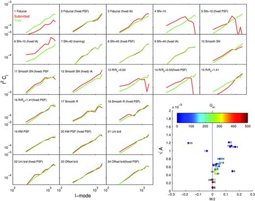
The true shear power (green) for each set and the shear power for the ‘fit2-unfold’ submission (red). The y-axes are C_ℓℓ² and the x-axis is ℓ. In the bottom right-hand corner, we show ⁠, and the colour scale represents the logarithm of the quality factor. The small numbers next to each point label the set number.

Open in new tabDownload slide

To investigate whether using high-S/N training data is useful for methods, we investigate a scenario where training on the power spectra had been used for all methods. This modification was potentially available to all participants if they chose to implement it. To do this, we measure the and values from the high-S/N Set 7 (see Table 2) and apply the transformation to the power spectra, which is to first order equivalent to an m and c correction,

9

to calibrate the method using the training data. In Fig. 3, we show the resulting quality factors when we apply both a denoising step and a training step and when we apply a training step only. When both steps are applied, we find that the quality factor improves by a factor of ≳2 and some methods perform as well as the ‘fit2-unfold’ method (if not better). In particular, ‘DEIMOS C6’ achieves an average quality factor of 316 (see Table 3). We find that the increase in the quality factor is uniform over all sets, including the low-S/N sets.

We conclude that it was a combination of model calibration on the data and using a denoised power spectrum that enabled ‘fit2-unfold’ to win the challenge. We also conclude that calibration of measurements on high-S/N samples, that is, those that could be observed using a deep survey within a wide/deep survey strategy, is an approach that can improve shape measurement accuracy by about a factor of 2. Note that using this approach is not doing shear calibration as it is practised historically because the true shear is not known. This holds as long as the deep survey is a representative sample and the PSF of the deep data has similar properties to the PSF in the shallower survey.

4.2.2 Multi-epoch data

In Fig. 3, we show how Q_dn varies for each submission averaged over all those sets that had a fixed intrinsic ellipticity field (Type 2) or a fixed PSF (Type 3), described in Section 3.1. Despite the simplicity of this implementation, we find that for the majority of methods, this variation, corresponding to multi-epoch data, results in an improvement of approximately 1.1–1.3 in Q_dn, although there is large scatter in the relation. In GREAT10, the coordination team made a decision to keep the labelling of the sets private, so that participants were not explicitly aware that these particular sets had the same PSF (although the functional PSFs were available) or the same intrinsic ellipticity field. These were designed to test stacking methods; however, no such methods were submitted. The approach of including this kind of subset can form a basis for further investigation.

In brief, we show in Fig. 4 how the population of the ⁠, and Q_dn parameters for each of the quantities that were varied between the sets, for all methods (averaging over all the other properties of the sets that were kept constant between these variations). In the following sections, we will analyse each behaviour in detail.

Figure 4

In each panel, we show the metrics, ⁠, and Q_dn, for each of the parameter variations between sets, for each submission; the colour scale labels the logarithm of Q_dn as shown in the lower right-hand panel. The first row shows the S/N variation, the second row shows the galaxy size variation, the third row shows the galaxy model variation (the galaxy models are: uniform bulge-to-disc ratios where each galaxy has a bulge-to-disc ratio randomly sampled from the bulge-to-disc ratio range [0.3, 0.95] with no offset (Uniform B/D No Offset), a 50 per cent bulge-to-disc ratio = 0.5 with no offset (50/50 B/D No Offset) and a 50 per cent bulge-to-disc ratio = 0.5 with a bulge-to-disc centroid offset (50/50 B/D Offset), and the fourth row shows PSF variation with and without Kolmogorov (KM) PSF variation.

Open in new tabDownload slide

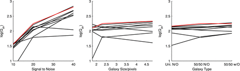
4.2.3 Galaxy signal-to-noise ratio

In the top row of Fig. 5, we show how the metrics for each method change as a function of the galaxy S/N. We find a clear trend for all methods to achieve better measurements on higher S/N galaxies, with higher Q values and smaller additive biases ⁠. In particular, ‘fit2-unfold’, ‘cat2-unfold’, ‘DEIMOS’, ‘shapefit’ and ‘KSB f90’ have a close-to-zero multiplicative bias for S/N > 20. Because S/N has a particularly strong impact, we tabulate the and values in Table 4. We also show in the lower row of Fig. 5 the breakdown of the multiplicative and additive biases into the components that are correlated with the PSF size and ellipticity (see Table 1). We find that for the methods with the smallest biases at high S/N (e.g. ‘DEIMOS’, ‘KSB f90’, ‘ARES’) the contribution from the PSF size is also small. For all methods, we find that the contribution from PSF ellipticity correlations is subdominant for ⁠.

Figure 5

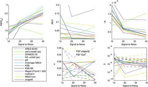
In the top panels, we show how the metrics, ⁠, and Q_dn, for submissions change as the S/N increases; the colour scale labels the logarithm of Q_dn. In the lower panels, we show the PSF size and ellipticity contributions α and β. In the bottom left-hand panel, we show the key that labels each method.

Open in new tabDownload slide

Table 4

Open in new tab

The metrics and for each of the S/N values used in the simulations.

Method	S/N= 10		S/N= 20		S/N= 40
†ARES 50/50	−0.028 320	0.140 511	−0.036 322	0.063 551	−0.006 060	0.034 517
†cat7unfold2 (ps)	−0.041 280	0.116 732	−0.002 803	0.058 890	0.001 880	0.016 527
DEIMOS C6	0.005 676	0.128 678	−0.006 533	0.061 440	0.017 020	0.021 269
fit2-unfold (ps)	0.148 242	0.093 275	−0.002 501	0.073 071	0.002 228	0.012 961
gfit	−0.033 046	0.123 692	0.026 172	0.045 710	0.019 359	0.026 773
*im3shape NBC0	−0.089 984	0.167 280	−0.068 486	0.071 842	−0.036 627	0.061 176
KSB	−0.065 856	0.175 017	−0.046 715	0.068 038	−0.024 967	0.046 845
*KSB f90	−0.009 688	0.147 320	0.005 480	0.065 486	−0.001 810	0.033 502
†MegaLUTsim2.1 b20	−0.380 576	0.224 465	−0.131 563	0.119 239	−0.174 472	0.117 005
method04	−0.099 330	0.168 536	−0.091 481	0.084 571	−0.077 907	0.048 824
†NN23 func	−0.009 595	0.086 018	0.015 145	0.104 664	0.072 641	0.152 932
shapefit	0.142 251	0.198 852	−0.003 768	0.070 808	0.001 568	0.033 164

Method	S/N= 10		S/N= 20		S/N= 40
†ARES 50/50	−0.028 320	0.140 511	−0.036 322	0.063 551	−0.006 060	0.034 517
†cat7unfold2 (ps)	−0.041 280	0.116 732	−0.002 803	0.058 890	0.001 880	0.016 527
DEIMOS C6	0.005 676	0.128 678	−0.006 533	0.061 440	0.017 020	0.021 269
fit2-unfold (ps)	0.148 242	0.093 275	−0.002 501	0.073 071	0.002 228	0.012 961
gfit	−0.033 046	0.123 692	0.026 172	0.045 710	0.019 359	0.026 773
*im3shape NBC0	−0.089 984	0.167 280	−0.068 486	0.071 842	−0.036 627	0.061 176
KSB	−0.065 856	0.175 017	−0.046 715	0.068 038	−0.024 967	0.046 845
*KSB f90	−0.009 688	0.147 320	0.005 480	0.065 486	−0.001 810	0.033 502
†MegaLUTsim2.1 b20	−0.380 576	0.224 465	−0.131 563	0.119 239	−0.174 472	0.117 005
method04	−0.099 330	0.168 536	−0.091 481	0.084 571	−0.077 907	0.048 824
†NN23 func	−0.009 595	0.086 018	0.015 145	0.104 664	0.072 641	0.152 932
shapefit	0.142 251	0.198 852	−0.003 768	0.070 808	0.001 568	0.033 164

Table 4

Open in new tab

The metrics and for each of the S/N values used in the simulations.

Method	S/N= 10		S/N= 20		S/N= 40
†ARES 50/50	−0.028 320	0.140 511	−0.036 322	0.063 551	−0.006 060	0.034 517
†cat7unfold2 (ps)	−0.041 280	0.116 732	−0.002 803	0.058 890	0.001 880	0.016 527
DEIMOS C6	0.005 676	0.128 678	−0.006 533	0.061 440	0.017 020	0.021 269
fit2-unfold (ps)	0.148 242	0.093 275	−0.002 501	0.073 071	0.002 228	0.012 961
gfit	−0.033 046	0.123 692	0.026 172	0.045 710	0.019 359	0.026 773
*im3shape NBC0	−0.089 984	0.167 280	−0.068 486	0.071 842	−0.036 627	0.061 176
KSB	−0.065 856	0.175 017	−0.046 715	0.068 038	−0.024 967	0.046 845
*KSB f90	−0.009 688	0.147 320	0.005 480	0.065 486	−0.001 810	0.033 502
†MegaLUTsim2.1 b20	−0.380 576	0.224 465	−0.131 563	0.119 239	−0.174 472	0.117 005
method04	−0.099 330	0.168 536	−0.091 481	0.084 571	−0.077 907	0.048 824
†NN23 func	−0.009 595	0.086 018	0.015 145	0.104 664	0.072 641	0.152 932
shapefit	0.142 251	0.198 852	−0.003 768	0.070 808	0.001 568	0.033 164

Method	S/N= 10		S/N= 20		S/N= 40
†ARES 50/50	−0.028 320	0.140 511	−0.036 322	0.063 551	−0.006 060	0.034 517
†cat7unfold2 (ps)	−0.041 280	0.116 732	−0.002 803	0.058 890	0.001 880	0.016 527
DEIMOS C6	0.005 676	0.128 678	−0.006 533	0.061 440	0.017 020	0.021 269
fit2-unfold (ps)	0.148 242	0.093 275	−0.002 501	0.073 071	0.002 228	0.012 961
gfit	−0.033 046	0.123 692	0.026 172	0.045 710	0.019 359	0.026 773
*im3shape NBC0	−0.089 984	0.167 280	−0.068 486	0.071 842	−0.036 627	0.061 176
KSB	−0.065 856	0.175 017	−0.046 715	0.068 038	−0.024 967	0.046 845
*KSB f90	−0.009 688	0.147 320	0.005 480	0.065 486	−0.001 810	0.033 502
†MegaLUTsim2.1 b20	−0.380 576	0.224 465	−0.131 563	0.119 239	−0.174 472	0.117 005
method04	−0.099 330	0.168 536	−0.091 481	0.084 571	−0.077 907	0.048 824
†NN23 func	−0.009 595	0.086 018	0.015 145	0.104 664	0.072 641	0.152 932
shapefit	0.142 251	0.198 852	−0.003 768	0.070 808	0.001 568	0.033 164

4.2.4 Galaxy size

In Fig. 6, we show how the metrics of each method change as a function of the galaxy size – the mean PSF size was ≃3.4 pixels. Note that the PSF size is statistically the same in each set, such that a larger galaxy size corresponds to either a case where the galaxies are larger in a given survey or a case where observations are taken where the pixel size and PSF size are relatively smaller for the same galaxies.

Figure 6

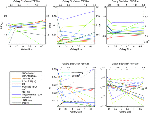
In the top panels, we show how the metrics, ⁠, and Q_dn, for submissions change as the galaxy size increases; the colour scale labels the logarithm of Q_dn. In the lower panels, we show the PSF size and ellipticity contributions α and β. In the bottom left-hand panel, we show the key that labels each method. The mean PSF is the mean within an image not between all sets.

Open in new tabDownload slide

We find that the majority of methods have a weak dependence on the galaxy size, but that at scales of ≲2 pixels, or size/mean PSF size ≃ 0.6, the accuracy decreases (larger and and smaller Q_dn). This weak dependence is partly due to the small (but realistic) dynamical range in size, compared to a larger dynamical range in S/N. The exceptions are ‘cat7unfold2’, ‘fit2-unfold’ and ‘shapefit’ which appear to perform very well on the fiducial galaxy size and less so on the small and large galaxies – this is consistent with the model calibration approach of these methods, which was done on Set 7 which used the fiducial galaxy type. The PSF size appears to have a small contribution at large galaxy sizes, as one should expect, but a large contribution to the biases at scales smaller than the mean PSF size. We find that the methods with largest biases have a strong PSF size contribution. Again the PSF ellipticity has a subdominant contribution to the biases for all galaxy sizes for ⁠.

4.2.5 Galaxy model

In Fig. 7, we show how each method’s metrics change as a function of the galaxy type. The majority of methods have a weak dependence on the galaxy model. The exceptions, similar to the galaxy size dependence, are ‘cat2-unfold’, ‘fit2-unfold’ and ‘shapefit’ which appear to perform very well on the fiducial galaxy model and less so on the small and large galaxies – this again is consistent with the model calibration approach of these methods. Again the contribution to from the PSF size dependence is dominant over the PSF ellipticity dependence, and is consistent with no model dependence for the majority of methods, except those highlighted here. We refer to Section 4.4 and Appendix E for a breakdown of m and c behaviour as a function of galaxy model for each method.

Figure 7

In the top panels, we show how the metrics, ⁠, and Q_dn, for submissions change as the galaxy model changes; the colour scale labels the logarithm of Q_dn. The galaxy models are: uniform bulge-to-disc ratio, each galaxy has, randomly sampled from the range [0.3, 0.95] with no offset (Uni.), a 50 per cent bulge-to-disc ratio = 0.5 with no offset (50/50.) and a 50 per cent bulge-to-disc ratio = 0.5 with a bulge-to-disc centroid offset (w/O). In the lower panels, we show the PSF size and ellipticity contributions α and β. In the bottom left-hand panel, we show the key that labels each method.

Open in new tabDownload slide

4.2.6 PSF model

In Fig. 8, we show the impact of changing the PSF spatial variation on the metrics for each method. We show results for the fiducial PSF, which does not include a Kolmogorov (turbulent atmosphere) power spectrum, and one which includes a Kolmogorov power spectrum in PSF ellipticity. We find that the majority of methods have a weak dependence on the inclusion of the Kolmogorov power. However, it should be noted that participants knew the local PSF model exactly in all cases.

Figure 8

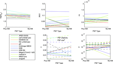
In the top panels, we show how the metrics, ⁠, and Q_dn, for submissions change as the PSF model changes; the colour scale labels the logarithm of Q_dn, the PSF models are the fiducial PSF, and the same PSF except with a Kolmogorov power spectrum in ellipticity added. In the lower panels, we show the PSF size and ellipticity contributions α and β. In the bottom left-hand panel, we show the key that labels each method.

Open in new tabDownload slide

4.3 Averaging methods

In order to reduce shape measurement biases, one may also wish to average together a number of shape measurement methods. In this way, any random component, and any biases, in the ellipticity estimates may be reduced. In fact the ‘ARES’ method (see Appendix E) averaged catalogues from DEIMOS and KSB and attained better quality metrics. Doing this exploited the fact that DEIMOS had in some sets a strong response to the ellipticity, whereas KSB had a weak response.

To test this, we averaged the ellipticity catalogues from the entries with the best metrics for each method that submitted an ellipticity catalogue (ARES 50/50, DEIMOS C6, gfit, im3shape NBC0, KSB, KSB f90, MegaLUTsim2.1 b20, method04, shapefit):

10

where i labels each galaxy and in general w_{m, i} is some weight that depends on the method, galaxy and PSF properties. We wish to weight methods that perform better, and so choose the quality factor from the high-S/N training set (Set 7) as the weight w_{m, i}=Q_{dn, m}(Set 7) applied over all other sets. This is close to an inverse variance weight on the noise induced on the shear power spectrum (⁠⁠). We leave the determination of optimal weights for future investigation.

We find that the average quality factors over all sets for this approach are Q= 131 and Q_dn= 210, which are slightly smaller on average than some of the individual methods. However, we find that for the fiducial S/N and large galaxy size the quality factor increases (see Fig. 9). This suggests that such an averaging approach can improve the accuracy of an ellipticity catalogue but that a weight function should be optimized to be a function of S/N, galaxy size and type; however, averaging many methods with a similar over- or under-estimation of the shear would not improve in the combination. If we take the highest quality factors in each set, as an optimistic case where a weight function had been found that could identify the best shape measurement in each regime, we find an average Q_dn= 393.

Figure 9

The quality factor as a function of S/N (left-hand panel), galaxy size (middle panel) and galaxy type (right-hand panel) for an averaged ellipticity catalogue submission (red, using the averaging described in Section 4.3), compared to the methods used to average (black).

Open in new tabDownload slide

4.4 Overall performance

We now list some observations of method accuracy for each method by commenting on the behaviour of the metrics and dependences discussed in Section 4 and Appendix E. Words such as ‘relative’ are with respect to the other methods analysed here. This is a snapshot of method performance as submitted for GREAT10 blind analysis.

• KSB. It has low PSF ellipticity correlations, and a small galaxy morphology dependence; however, it has a relatively large absolute m bias value.

• KSB f90. It has small relative m and c biases on average, but a relatively strong PSF size and galaxy morphology dependence, in particular on the galaxy bulge fraction.

• DEIMOS. It has small m and c biases on average, but a relatively strong dependence on galaxy morphology, again in particular on the bulge fraction, similar to KSB f90. Dependence on galaxy size is low except for small galaxies with size smaller than the mean PSF.

• im3shape. It has a relatively large correlation between PSF ellipticity and size, a small galaxy size dependence for m and c but a stronger bulge fraction dependence.

• gfit. It has relatively small average m and c biases, and a small galaxy morphology dependence; there is a relatively large correlation between PSF ellipticity and biases m and c. This was the only method to employ a denoising step at the image level, suggesting that this may be partly responsible for the small biases.

• method 4. It has relatively strong PSF ellipticity, size and galaxy type dependence.

• fit2-unfold. It has strong model dependence, but relatively small m and c biases for the fiducial model type, and also a relatively low correlation between PSF ellipticity and m and c biases.

• cat2-unfold. It has strong model dependence, in particular, on galaxy size, but relatively small m and c biases for the fiducial model type, and also a relatively low PSF ellipticity correlation.

• shapefit. It has a relatively low quality factor, and a strong dependence on model types and size that are not the fiducial values, but small m and c biases for the fiducial model type.

To make some general conclusions, we find the following:

• Signal-to-noise ratio. We find a strong dependence of the metrics below S/N= 10 especially for additive biases; however, we find methods that meet bias requirements for the most ambitious experiments when S/N > 20.

• Galaxy type. We find marginal evidence that model-fitting methods have a relatively low dependence on galaxy type compared to KSB-like methods, but that this is only true if the model matches the underlying input model (note that GREAT10 used simple models). We find evidence that if one trains on a particular model, then biases are small for this subset of galaxies.

• PSF dependence. Despite the PSF being known exactly, we find contributions to biases from PSF size, but less so from PSF ellipticity. The methods with the largest biases have a strong PSF ellipticity–size correlation.

• Galaxy size. For large galaxies well sampled by the PSF, with scale radii ≳2 times the mean PSF size, we find that methods meet requirements on bias parameters for the most ambitious experiments. However, if galaxies are unresolved with scale radii ≲1 time the mean PSF size, the PSF size biases become significant.

• Training. We find that calibration on a high-S/N sample can significantly improve a method’s average biases. This is true irrespective of whether training is a model calibration or a more direct form of training on the ellipticity values of power spectra themselves.

• Averaging methods. We find that averaging methods are clearly beneficial, but that the weight assigned to each method needs to be correctly determined. An individual entry (ARES) found that this was the case, and we find similar conclusions when averaging over all methods.

Note that statements on required accuracy are only on biases, and not on the statistical accuracy on shear that a selection in objects with a particular property (e.g. high S/N) would achieve. Such selection is dependent on the observing conditions and survey design for a particular experiment, so we leave such an investigation for future work.

5 ASTROCROWDSOURCING

The GREAT10 Galaxy Challenge was an example of ‘crowdsourcing’ astronomical algorithm development (‘astrocrowdsourcing’). This was part of a wider effort during this time period, which included the GREAT10 Star Challenge and the sister project Mapping Dark Matter (MDM)5 (see companion papers for these challenges). In this section, we discuss this aspect of the challenge and list some observations.

GREAT10 was a major success in its effort to generate new ideas and attract new people into the field. For example, the winners of the challenge (authors DK and DM) were new to the field of gravitational lensing. A variety of entirely new methods have also been attempted for the first time on blind data, including the Look Up Table (MegaLUT) approach, an autocorrelation approach (method04 and TVNN), and the use of training data. Furthermore, the TVNN method is a real pixel-level deconvolution method, a genuine deconvolution of data used for the first time in shape measurement.

The limiting factor in designing the scope of the GREAT10 Galaxy Challenge was the size of the simulations which was kept below 1 TB for ease of distribution; a larger challenge could have addressed even more observational regimes. In the future, executables could be distributed that locally generate the data. However, in this case, participants may still need to store the data. Another approach might be to host challenges on a remote server where participants can upload and run algorithms. However, care should be taken to retain the integrity of the blindness of a challenge, without which results become largely meaningless as methods could be tuned to the parameters or functions of specific solutions if those solutions are known a priori. We require algorithms to be of high fidelity and to be useful on large amounts of data, which requires them to be fast: an algorithm that takes a second per galaxy needs ≃50 CPU years to run on 1.5 × 10⁹ galaxies (the number observable by the most ambitious lensing experiments e.g. Euclid,6Laureijs et al. 2011); a large simulation generates innovation in this direction.

In Fig. 10, we show the cumulative submission of the GREAT10 Galaxy Challenge as a function of time, from the beginning of the challenge to the end and in the post-challenge submission period. All submissions (except one made by the GREAT10 coordination team) were made in the last 3 weeks of the 9 month period. For future challenges, intrachallenge milestones could be used to encourage early submissions. This submission profile also reflects the size and complexity of the challenge; it took time for participants to understand the challenge and to run algorithms over the data to generate a submission. For future challenges, submissions on smaller subsets of data could be enabled, with submission over the entire data set being optional.

Figure 10

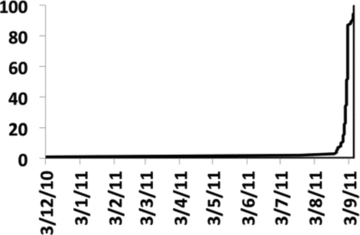
The cumulative submission number as a function of the challenge time, which started on 2010 December 3 and ran for 9 months.

Open in new tabDownload slide

We note that the winning team (DK and DM) made 18 submissions during the challenge, compared to the mean submission number of 9. The winners also recognized from the information provided that the submission procedure was open to power spectrum and ellipticity catalogue submissions. The leaderboard was designed such that accuracy was reported in a manner that was indicative of performance, but that this information could not be trivially used to directly calibrate methods (e.g. if m and c were provided a simple ellipticity catalogue submission, correction could have been made).

Many of these issues were overcome in the sister MDM challenge (see the MDM results paper, Kitching et al., in preparation) which received over 700 entries, over 2000 downloads of the data and a constant rate of submission. It also used an alternative model for leaderboard feedback where the simulated data were split into public and private sets, and useful feedback was provided only for the public sets.

For a discussion of the simplifications present in GREAT10, we also refer the reader to sections 5 of the GREAT10 Handbook (Kitching et al. 2011).

6 CONCLUSIONS

The GREAT10 Galaxy Challenge was the first weak-lensing shear simulation to include variable fields: both the PSF and the shear field varied as a function of position. It was also the largest shear simulation to date, consisting of over 50 million simulated galaxies, and a total of 1 TB of data. The challenge ran for 9 months from 2010 December to 2011 September, and during that time approximately 100 submissions were made.

In this paper, we define a general pseudo-C_ℓ methodology for propagating shape measurement biases into cosmic shear power spectra and use this to derive a series of metrics that we use to investigate methods. We present a quality factor Q that relates the inaccuracy in shape measurement methods to the shear power spectrum itself. Q= 1000 denotes a method that could measure the dark energy equation-of-state parameter w₀ with a bias less than or equal to the predicted statistical error from the most ambitious planned weak-lensing experiments (for a more general expression, we refer to Massey et al., in preparation). We show how one can correct such a metric to account for pixel noise in a shape measurement method. During the challenge, submissions were publicly ranked on a live leaderboard and ranked by this metric Q.

We show how a variable shear simulation can be used to determine the m and c parameters (Heymans et al. 2006) which are a measure of bias between the measured and true shear (those parameters used in constant shear simulations, STEP and GREAT08) on an object-by-object basis. We link the quality factor to linear power spectrum biases including a multiplicative and additive bias that are approximately related to the STEP one-point estimators of shape measurement bias. The equality is only approximate because in general and are a measure of spatially varying method biases. We introduce further metrics that allow an assessment of the contribution to the multiplicative and additive biases from correlations between the biases and any spatially variable quantity (in this paper, we focus on PSF size and ellipticity).

The simulations were divided into sets of 200 images each containing a grid of 10 000 galaxies. In each set, the shear field was spatially varying but constant between images. The challenge was to reconstruct the shear power spectrum for each set. Participants could submit either catalogues of ellipticities, one per image, or power spectra, one for each set, and were provided with an exact functional description of the PSF and the positions of all objects to within half a pixel.

The simulations were structured in such a way that conclusions could be made about a shape measurement method’s accuracy as a function of galaxy S/N, galaxy size, galaxy model/type and PSF type. The simulations also contained some ‘multi-epoch’ sets in which the shear and intrinsic ellipticities were fixed between images in a set but where the PSF varied between images, and some ‘static single-epoch’ sets where the PSF was fixed between images in a set but the intrinsic ellipticity field varied between images. All fields were always spatially varying. Participants were provided with true shears for one of the high-S/N sets that they could use as a training set.

Despite the simplicity of the challenge, making conclusions about which aspects of which algorithm generated accurate shape measurement is difficult due to the complexity of the algorithms themselves (see Appendix E). We leave investigations into tunable aspects of each method to future work. We can, however, make some statements about the regimes in which methods perform well or poorly.

The best methods submitted to GREAT10 scored an average Q≃ 300 with m≃ 7 × 10⁻³ and c≃ 10⁻⁵. The best performing non-stacking method at S/N= 20, using the GREAT10/SExtractor definition, in GREAT08 was KSBf90 (CH) which had an m= 0.0095 ± 0.003 and c≃ 8 × 10⁻⁴, and we find a similar performance on GREAT10. Comparing this benchmark against methods here, we find at least a factor of 3 improvement in performance by methods tested on blind simulations (we refer to Table 3 where the mean improvement over KSBf90 is 2.6 ± 1.6 over all metrics). The methods that won the challenge (scoring the highest Q on the leaderboard) employed a maximum-likelihood model-fitting method. Several methods used the training data to test code, and we find that by directly training on a high-S/N set the majority of methods achieve a factor of 2 increase in the average value of Q. We find some evidence that shape measurement inaccuracies can be reduced by averaging methods together, but conclude that for such a method to be useable an optimal weight for each method as a function of S/N and galaxy properties would have to be found.

For S/N of 40 the best methods achieved Q≳ 1000, m < 1 × 10⁻³ and c < 1 × 10⁻⁵; the majority of methods have an accuracy that is strongly dependent on S/N with Q≃ 100 and ≃50 for S/N of 20 and 10, respectively. However, the dependence on galaxy model (bulge-to-disc ratio or bulge-to-disc offset) and size is not strong. There is a contribution to the multiplicative bias m from PSF ellipticity–size correlations for the majority of methods over all sets, but a smaller contribution from PSF ellipticity dependence (as expected from theoretical calculations e.g. Massey et al., in preparation).

The testing of shape measurement methods by GREAT10 suggests methods now exist which can be used for cosmic shear surveys covering up to a few thousand square degrees (≲3000 deg², that require m≲ 6 × 10⁻³; Kitching et al. 2008,7) to measure cosmological parameters in an unbiased fashion. We find that on the additive bias c methods already meet requirements for even the most ambitious surveys (c < 1 × 10⁻³) over all simulated conditions, and that in the high-S/N regime (≳40) methods already meet the most ambitious requirements on the multiplicative bias (m < 2 × 10⁻³; Kitching et al. 2008). Now that such accuracy has been demonstrated in the high-S/N regime, it is now plausible that such accuracy may be possible at lower S/N, in principle. However, we note that the requirements are on all galaxies in a survey and that the demonstration here is averaged over a simulation with particular properties, in particular, the fiducial S/N is 20. Therefore, these conclusions have a caveat that the GREAT10 simulations were intentionally simplistic in some respects, so that clear statements about methods could be made, but they provide a foundation for shape measurement development to continue to increase in realism and complexity.

We thank the GREAT10 Advisory team for discussions before and after the challenge. TDK is supported by a Royal Society University Research Fellowship, and was supported by a Royal Astronomical Society 2010 Fellowship for the majority of this work. This work was funded by a EU FP7 PASCAL 2 Challenge Grant. Workshops for the GREAT10 challenge were funded by the eScience STFC Theme, PASCAL 2 and JPL, run under a contract for NASA by Caltech, and hosted at the eScience Institute Edinburgh, by UCL and IPAC at Caltech. We thank Bob Mann, Francesca Ziolkowska, Harry Teplitz and Helene Seibly for local organization of the workshops. We thank Mark Holliman for system administrator tasks for the GREAT10 web server. We thank Whitney Clavin for assistance on the NASA press release for GREAT10. We thank Lance Miller comments on a first draft and throughout the challenge. We also thank Alan Heavens, Alina Keissling, Benjamin Joachimi, Marina Shmakova, Gary Bernstein, Konrad Kuijken, Yannick Mellier, Mark Cropper, Malin Velander, Elisabetta Semboloni, Henk Hoekstra and Karim Benabed for useful discussions. CH acknowledges support from the ERC under grant EC FP7 240185. SB, MH, TK, BTPR and JZ acknowledge support from an ERC Starting Grant with number 240672. BTPR acknowledges support from the NASA WFIRST Project Office. DK and DM acknowledge the support of the US DOE. RJM acknowledges support from a Royal Society University Research Fellowship. We thank an anonymous referee for helpful comments that improved the analysis and clarity of this paper.

Contributions: All authors contributed to the development of this paper. TDK was PI of GREAT10, created the simulations, and wrote this paper. CH, MG, RJM and BTPR were active members of the GREAT10 coordination board during the challenge (2010 December to 2011 October). SB, FC, MG, SH, CH, MH, TK, DK, DM, PM, GN, KP, BTPR, MT, LV, MV, JY and JZ submitted entries to the GREAT10 galaxy challenge. JR hosted and ran the GREAT10 challenge final workshop, and TDK, CH, SB, MH, TK, RJM, BTPR, LV and JZ were on the LOC for the mid-challenge workshops. STB and SB created the image simulation code for GREAT08 which was extended by TDK for the GREAT10 challenge. ANT contributed to the code on which the spatially varying field code was based, and provided consultation with regard to the pseudo-C_ℓ formalism. DW maintained the GREAT10 leaderboard and processed submissions with TDK during the challenge.

Footnotes

REFERENCES

Appendices

APPENDIX A: Pseudo-C_ℓ ESTIMATORS FOR WEAK LENSING

In this section, we describe a formalism for the evaluation of variable shear systematics in weak lensing. We note that this has a more general application than that described here, such that any mask in general could be accounted for in weak-lensing power spectrum estimation. This closely follows the pseudo-C_ℓ formalism described in Memari (2010) and Brown, Castro & Taylor (2005) which has been applied in cosmic microwave background studies, for survey masks.

We start by defining a generalized shear systematic response where

(A1)

where all variables are a function of position on the sky, and all are complex quantities (e.g. ⁠). We expect that will in general depend on spatially varying quantities including PSF ellipticity and size or galaxy properties such as S/N, so that one could write or for example, but this does not qualitatively change the following treatment. We note also that in general the systematic terms can also be complex, ⁠, where we assume a scalar spatially varying quantity, and will investigate further generalization in future work.

The E- and B-mode decomposition of the spin-2 field can be written in general as a rotation in Fourier space (see GREAT10 handbook) such that

(A2)

where is the Fourier transform of ⁠.

When creating a power spectrum, the autocorrelations of the first three terms of equation (A1) have a simple interpretation, but the fourth term has an effective weight map as a function of position such that (only focusing on the contribution from the fourth term) the estimated E- and B-mode terms are

(A3)

where W_m is 2D Fourier transform of the field. Equivalently for the E-mode part only we have

(A4)

where this equation has the interpretation of a rotation of E and B to ellipticity in Fourier space, a convolution with the window/weight function and then a rotation back to E and B. We now wish to compute the effect that the weight map has on the E-mode power. In Fourier space, the auto-power and cross-power are defined as

(A5)

where isotropy of the field is assumed. This means that an unbiased estimator can be written in the flat sky limit as an average over angle in ℓ space:

(A6)

Hence by taking the correlation function of equation (A4) we can calculate the estimated power spectrum in the presence of a systematic weight map. This follows the calculations of Memari (2010); the resulting expressions for the EE power and BB power are given below, and we include the EB expression for completeness (however, in the flat sky limit, there is no EE, BB and EB mixing; there is between EE and BB though):

(A7)

where the additional L mode forms a triangle with ℓ and ℓ′ (|ℓ−ℓ′| < L < ℓ+ℓ′) with cos η= (ℓ²+ℓ′²−L²)/2ℓℓ′ and similarly for sin η, and W_mm is the angle average of the modulus squared of the weight function

(A8)

In the discrete case, we can write equations (A7) in a compact form using mixing matrices such that

(A9)

where

(A10)

and similarly for the EB power; Δℓ′ is the separation between the discrete ℓ′ modes. These expressions assume that the systematic fields are uncorrelated with the shear and intrinsic ellipticity fields. This may not be the case in real data (e.g. selection effects over galaxy populations may have particular biases), but for GREAT10 selection effects are not investigated and the biases are quoted as averages over populations. We leave a generalization of this formalism to correlated systematic-ellipticity fields for future work.

Using this we can write a power spectrum estimate of the quantities in equation (A1) (we drop the angular brackets over φ_ℓ for clarity) including the γI cross-term as

(A11)

where is the angle-averaged power spectrum of the variation; here, through isotropy, it is assumed that the power contains all relevant information. This could be generalized to include non-isotropic variation in all terms, that is, not taking the angle averages. m_ℓ is the angle-averaged Fourier transform of ⁠. Our notation, for example, ⁠, refers to the EE power corresponding to correlations between quantities A and B as a function of ℓ. We do not include terms from the quadratic contribution. For GREAT10, the γ field is E mode only and the intrinsic ellipticity field is B mode only, with no γI term, so we have a simpler expression

(A12)

These expressions are general for a wide class of shape measurement biases, and are trivially extendable, for example, to include cross-terms that may appear in real data (e.g. 〈cm〉 cross terms), if required.

Equation (A12) represents in general how shape measurement inaccuracies in GREAT10 can propagate through to the shear power spectrum. In the case that the weight map is constant [⁠, and with some associated error σ(c)], the Fourier transform becomes a delta function and the mixing matrices become and ⁠. This leads to

(A13)

where and are constant functions of scale. In general, the mixing matrices are not only dependent on a single ℓ (i.e. diagonal M_ℓℓ) except in the case that the systematic is isotropic or constant. Unfortunately, this is likely not to be the case in weak lensing where, for example, PSF ellipticity and size are often coherent but not constant across a field of view. Massey et al. (in preparation) will discuss requirements on these parameters, and ⁠, and how they relate to uncertainty in PSF parameters.

We note that this formalism means that we only need to recover the statistical properties of the varying field (the power spectrum and mixing matrix) in order to propagate its impact through to the shear power spectrum. In addition, as shown in Appendix B, this formalism can also be used to generate expressions for correlation coefficients between the systematic and fields and any spatially varying quantity. Given these definitions and formalisms, we can now proceed to outline the metrics used in this paper, taking into account some practicalities such as pixel noise removal.

Appendix B: DESCRIPTION OF THE EVALUATION METRICS

The variable shear nature of the simulations enables a variety of metrics to be calculated, each of which allows us to infer different properties of the shape measurement method under scrutiny. In this paper, we define a variety of metrics that we explain in detail in this section.

B1 Quality factor

In general for a variable field we define the power spectrum as the Fourier transform of the correlation function as described in Appendix A. We wish to compare the power reconstructed from the submissions against the true shear power spectrum and so define a baseline evaluation metric, the quality factor (Q), as

(B1)

The numerator 5 × 10⁻⁶ is calculated by generating Monte Carlo realizations of a mock submitted power spectrum and calculating the bias in the dark energy equation-of-state parameter w₀ (Linder 2003) which would occur if such an observation were made (using the functional form filling formalism described in Kitching et al. 2009) over a survey of 20 000 deg² using the same redshift distribution as described in Section 3.2. In Fig. B1 we show the result of this procedure for GREAT10 [where the numerator in equation (B1) is labelled as ], where we take a threshold value of bias-to-error ratio of 1. This is in fact conservative as shown in Massey et al. (in preparation). The factor of 1000 normalizes the metric such that a good method should achieve Q≃ 1000. A factor could be included in the denominator, but we absorb this into the factor 5 × 10⁻⁶. This was the quality factor used in the online leaderboard during the challenge.

Figure B1

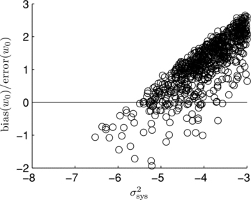
Monte Carlo realizations of submitted shear power spectrum where is the denominator in equation (B1), and the calculated bias in dark energy parameter with respect to its error.

Open in new tabDownload slide

B2 Pixel-noise-corrected quality factor

In general we can express the measured total ellipticity by including a noise term in equation (A1), where e_n is some inaccuracy in this estimator due to stochastic terms in shape measurement methods, or due to pixel noise in the images (finite S/N). In the simulations, for ellipticity catalogue submissions, we averaged over N_realization realizations of the noise. In this averaging, the mean of the noise contribution is assumed to be zero, 〈e_n〉= 0, over realizations, but where there is an error on this mean that remains. By propagating this through to the power spectrum, we recover

(B2)

where the noise term is white noise (constant over all scales) with a variance ⁠, which is a sum of the e₁ and e₂ components. The noise term is now averaged over the number of realizations and the number of objects. For values of N_realization= 200 and N_object= 10⁴ the expected fractional contribution to the measured power ⁠.

The measured power spectra inferred from the ellipticity catalogue submissions and used in the quality factor (Q) defined in equation (B1) therefore include this noise term. However, for an error induced by noise on ellipticity estimates of σ≲ 0.05 the impact on the metric should be subdominant. It is commonly assumed that such noise terms could be removed in real data (this is trivial for correlation functions, but is more complex for power spectrum estimates; that requires an estimate of σ_n from data – the full covariance of the shear estimators, see also e.g. Schneider, Eifler & Krause 2010), and some power spectrum submissions (see Section E) did employ techniques to remove this term from the submitted power spectrum. Hence, we here introduce a quality factor that accounts for this noise term,

(B3)

where is an estimated value of the pixel noise term from the ellipticity catalogue submissions.

To estimate the value of from the simulations, we have to separate the E-mode shear field from the B-mode-only intrinsic ellipticity field; otherwise, the variance of the ellipticities from a submitted entry will be dominated by the variance of the intrinsic ellipticities. This is done using the rotations described in Appendix A; here, we describe this pedagogically. [We also use explicit Cartesian coordinates and for clarity.] We make a 2D discrete Fourier transform of the submitted ellipticity values such that

(B4)

where the measured ellipticity is averaged over all noise realizations before transformation. We then rotate this field such that

(B5)

and then inverse Fourier transform to real space

(B6)

where we now have a κ(x, y) field which contains E-mode power only and a β(x, y) field that contains B-mode power only. The simulations have been set up such that the intrinsic ellipticity field has B-mode power only, such that we can now take the κ(x, y) map and generate an E-mode-only ellipticity catalogue that should only contain the estimated shear values and the noise term:

(B7)

where is the estimate shear for each position (object) in field. We do this by following the inverse steps of transformations from equations (B4) to (B6), and assume noise is equally distributed between E and B modes. The expression is only approximate because of position-dependent biases (see Appendix A and section B5), which can mix E and B modes, but for the majority of methods presented in this paper this effect seems to be subdominant. By taking the normal variance of e_{E, measure}(x, y) we find that

(B8)

and so our estimate of the noise variance is

(B9)

To calculate this we use the true shear values to find ⁠; this is unrealistic but note that the true individual shear values are not used directly only to calculate the variance. For real data, as done by ‘fit2-unfold’ we expect that noise estimates from each galaxy will be used to calculate this correction. Indeed part of the challenge, demonstrable by the ‘fit2-unfold’ submissions, was to develop optimal estimates for ⁠.

To test that such a correction works, we simulated a submission by taking the true shear values and adding random normally distributed numbers to each of the 10 000 × 200 × 24 shear values. We show results in Fig. B2. We find as expected that as the noise increases, the value of Q (equation B1) decreases, but that including the noise correction (equation B3) increases the value. Note that due to the finite size of the simulations any estimation of is itself noisy which means the corrected value of Q_dn < ∞ even in this ideal case.

Figure B2

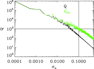
A simulation of the effect on Q (black line) and Q_dn (green line) as the noise in a mock submission (containing only noise and the true shear values) increases. Lines at Q= 1000 and σ_n= 0.1 are to guide the reader.

Open in new tabDownload slide

B3 One-point estimator shear relations

As well as metrics that integrate over the measured power spectra, we can also investigate a number of metrics that encapsulate a relation between the measured and true shears for individual objects. This ties the quality factor metrics to the STEP (Heymans et al. 2006) m and c values where

(B10)

where is the true shear and is the measured shear for each component; this is a simplification of equation (A1), and that used for all constant shear simulations (with no position dependence). We also add a quadratic non-linear term to this relation (⁠⁠):

(B11)

which contains γ|γ|, not γ², since we may expect divergent behaviour to more positive and more negative shear values for each domain, respectively. In general m_ij and q_ij could be non-diagonal matrices; however, in this paper, we assume that they are diagonal and take an average over the two shear components to give

(B12)

where all quantities are averaged over γ₁ and γ₂.

In a variable shear simulation, calculating m, c and q by regressing e_measure and (γ+e_intrinsic) would result in a noisy estimator dominated by intrinsic ellipticity noise. However, we can calculate m, c and q directly by finding the estimated shear for each galaxy individually, removing the intrinsic ellipticity contribution (equation B7). This is for every galaxy a noisy estimate of the shear; we then average these estimates over bins in γ^t. This enables the m, c and q parameters to be recovered, and in fact the variable field simulations allow for a flexible binning as a function of any other spatially varying quantity (see Appendix E), and an exact removal of shape noise (through the B-mode intrinsic power). This method of calculating the m, c and q parameters is a one-point estimate of the shape measurement biases and makes no assumption about spatially correlated effects.

B4 Power spectrum relations

As described in Appendix A, we can write an expression for the estimated power using two linear parameters and ⁠, taking into account the pixel noise removal,

(B13)

This can be related to the m and c parameters:

(B14)

where σ(c) is the variance of the c parameter, but only approximately because of the assumption of some form of spatial variation (constant in this case).

In Fig. B3 we show how Q_dn, ⁠, and the point estimators m and c are related. To create this, we explore the (⁠⁠, ⁠) plane and using the fiducial power spectrum calculate Q_dn for each value. We also show a realization where random components have been added, where R is a uniform random number, and similarly for ⁠, at each point in parameter space to simulate a more realistic submission. We find that there is a degenerate line in Q_dn where an offset can be partially cancelled by a negative yielding the same Q_dn, and a more straightforward relation for ⁠. As expected, the c parameter does not impact the quality factor but the variance of c does. There is a similar degeneracy among m, σ(c) and Q_dn to that among the linear power spectrum parameters, as expected from equation (B14), except that for large negative m the quadratic m² term begins to become important.

Figure B3

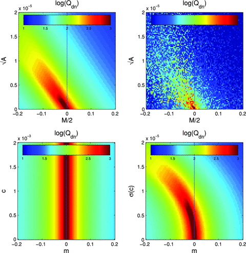
An exploration of the (⁠⁠, ⁠), (m, c) and (m, σ(c)) planes, where at each point the quality factor is calculated using a noise-free fiducial power spectrum. The colour scale shows the logarithm of the quality factor. This can be compared to Fig. 2.

Open in new tabDownload slide

B5 Correlations with spatially varying quantities

To relax the assumption of constant m and c in power spectrum analysis, we can assume that each of these is correlated with some spatially varying parameter ⁠:

(B15)

with the correlation coefficients α and β; X₀ is a constant reference value to ensure that the units of α and β are dimensionless: for ellipticity, this is set to unity, and for PSF size squared, this is the mean PSF size squared. This is a simple relation and could be made significantly more complex.

We explain in a correlation function notation how these propagate through, for pedagogical purposes, but for the full treatment one should refer to the pseudo-C_ℓ methodology which we present in Appendix A. A simple correlation function approximation of the measured shear can be written as

(B16)

not including the pixel noise term. We can also take the cross-correlation between the measured ellipticity and these quantities:

(B17)

which results in an expression that is not dependent on α, assuming that third-order correlations and noise–X correlations are zero.

The corresponding full expressions for the pseudo-C_ℓ power spectrum, including the noise correction term (which we assume is uncorrelated with all other terms), are

(B18)

The second expression has cross-power spectra on both sides. The matrices M^XX are the mixing matrices for the spatially varying quantity X. In general, the variation of X is not isotropic – PSF ellipticity, for example, can have a preferred direction in an image; however, here we make the assumption of isotropy in defining the power ⁠.

To calculate these from the simulations, we find the best-fitting α and β values (using a minimum least-squares estimator over the ℓ range defined in Appendix E) for X= PSF size squared and PSF ellipticity. Because this calculation is done on sets that are averaged over noise realizations, this can only be calculated for those sets in which the PSF is fixed for a set (for the PSF correlations).

The relation to the linear power relations and is not straightforward because of the non-diagonal mixing matrix in general. Therefore, in the results section (Section 4), we will quote values for the correlation coefficients α_e, ⁠, β_e, for ellipticity and PSF size squared (the square of the size is the most relevant quantity for propagated PSF-shear behaviour, see Massey et al., in preparation and Paulin-Henriksson et al. 2008). Note that α and β are unitless and scaled by a reference value X₀= [〈X〉]: for PSF size correlations, this means units of X₀= 3.4²= 11.56 pixel², and for ellipticity correlations the quantities are unitless, X₀= 1. If one were to expand the bias in terms of a different scaling, a natural expansion one may use, for example, is as a function of R_PSF/R_galaxy, and then a scaling can be applied to results presented in this paper.

APPENDIX C: SIMULATION MODELLING

In this section, we provide some further details of the variable shear and PSF field, as well as the local modelling of the galaxies and stars.

C1 Scaling of the shear field

We note that in performing the process of sampling the shear field discretely and then generating a postage stamp for each sampling the inter-postage stamp separation in the final image has a distance of θ_image/100, but this is not necessarily related to the pixel scale of the postage stamps, that is, in general. As a result, the number density of the galaxies can be scaled as

(C1)

and the maximum ℓ set by the grid separation of the galaxies scales as

(C2)

where 100 is the number of grid positions on a side. However, note that the true underlying simulated shear field is always fully sampled in every case.

For the case of θ_image= 10°, this gives values of n₀= 0.0277 and ℓ_max= 1800. The images, however, can be scaled to match a variety of other configurations, with the caveat that the absolute value of the shear power is constant; θ_image= 1° gives a scaling of n₀= 2.77 and ℓ_max= 18 000, and θ_image= 0°.5 gives a scaling of n₀= 11.1 and ℓ_max= 36 000. In each case the absolute amplitude of the calculated shear power also needs to be scaled. It is then fair to match the simulations to either of these cases, which span a reasonable expected dynamical range in the number density of objects but with a coupled increase in the maximum ℓ range. The ℓ values used for the Q metrics are ℓ= (233, 415, 600, 789, 977, 1162, 1350, 1538). These are specified as follows: (i) defining the maximum and minimum ℓ modes, we do not generate ℓ modes above that corresponding to the grid separation, and avoid the smallest ℓ modes where the S/N is low; (ii) we choose eight bins linearly spaced in ℓ between these limits; (iii) we define a grid in (ℓ_x,ℓ_y) for the power spectrum calculation, defined with Δℓ= 36; and (iv) we integrate over this grid and take the mean ℓ value from the grid points in each of the eight ℓ bins. The bins were originally defined under the assumption that an equivalent accuracy of Q≳ 1000 in each ℓ bin independently is desirable; see Fig. B2 where, given the size of the simulation (200 noise realizations), and assuming that σ_n∼ 0.01 for a good method, we find Q∼ 1000 at ⁠, although this is only an estimated number for any given method. Eight ℓ bins were also defined for computational speed. We caution here that accuracy statements will be dependent on the maximum and minimum ℓ ranges, and on the shape of the power spectrum in general.

We could replace the integrals in the Q factor definitions with sums for the discrete ℓ case where ∫dℓ→∑_{ℓ= (233, 415, 600, 789, 977, 1162, 1350, 1538)}Δℓ, but we keep the integral version in the text to maintain a general expression and for clarity. The power C^EEℓ² is binned, and compared to the binned equivalent of the true/input power spectrum – the power spectrum of the actual realization of the shear field – calculated in exactly the same way as the submitted power (one may refer to this as the ‘sample’ input power spectrum).

C1.1 ℓ integration

Here we briefly discuss a technical issue with regard to the ℓ integral accuracy used for the Q factor calculation. The Q value is defined via

(C3)

with Q_N= 0.005 and

(C4)

We can rewrite equation (C3) without any approximations as

(C5)

For concreteness, we assume equally spaced bins that are linear in ℓ: ℓ_i≡ℓ_min+iΔℓ with i= 1, 2, …, N_bins and Δℓ= (ℓ_max−ℓ_min)/N_bins. We calculate the integral over the difference in the power using Monte Carlo integration of the average value of for ℓ_{i− 1} < ℓ≤ℓ_i based on the ellipticities associated with a single realization of ⁠, and similarly for ⁠. Therefore, we have a quantity that is related to I_i which can be written as

(C6)

Working to second order in Δℓ to evaluate different schemes for estimating the value of equation (C3), we have

(C7)

with

(C8)

then

(C9)

and

(C10)

We are now in a position to calculate the numerical approximation errors inherent in different schemes for combining values of to estimate the value of equation (C3).

Linear scheme

A straightforward implementation of the integration over ℓ in equation (C3) in terms of a finite sum yields 1/ℓ_{i− 1/2} weights and is accurate to second order:

(C11)

Log scheme

We can also implement the integration over log ℓ (first equality in equation C3) as a straightforward finite sum approximation, which implies log (ℓ_i/ℓ_{i− 1})/Δℓ weights and is also formally accurate to second order:

(C12)

Comparing the two schemes above, both are accurate to second order (there are further schemes that are only accurate to first order). In order to compare the two methods, we need to assume something about how the error in each bin, ⁠, grows with ℓ, and then compare

(C13)

Suppose that the leading term in the Taylor expansion of f(ℓ) is cℓⁿ, then we can calculate the leading behaviour for the ratio of equation (C11) to (C12) explicitly as

(C14)

Therefore, we conclude that the linear scheme is generally more accurate, and that the log scheme is only competitive in the unlikely scenario that f(ℓ) depends very strongly on ℓ. Since we find empirically that f(ℓ) ∝ℓ² (i.e. is approximately constant over bins), n= 2 is a good approximation and the linear scheme is then roughly twice as accurate as the log scheme.

C2 The galaxy models

Here we describe how the individual galaxies are modelled. Each galaxy is composed of a bulge and a disc, defined as radial intensity profiles with

(C15)

where K= 2n− 0.331 with n= 4 for the bulge and n= 1 for the disc and i={b, d} for bulge and disc, respectively. Both are Sérsic profiles (the latter being an exponential profile). The intensity is normalized to match the S/N, and the scale radii for the disc and bulge, r_d and r_b, respectively, are in general free parameters; fiducial values for these parameters were set to be r_b= 2.3 and r_d= 4.8 pixels. In Bridle et al. (2010), and for the code used for this challenge, the values of radii r are the half-light radius for both bulges and discs. The disc exponential scalelengths and half-light scale radii differ by a factor of 1.669.

In most sets, the size distribution over objects was a compact Gaussian, with a variance of σ_R= 0.01:

(C16)

and similarly for the disc distribution. In three sets (see Section 3.1), the galaxy size varied for each galaxy in the set; in these cases, the functional form for the S/N variation was a Rayleigh distribution:

(C17)

where σ_R= 2.0 for these sets, and r_b and r_d are the fiducial values. There is a caveat that the sizes referred to here (and in the GREAT08 simulations) refer to the pre-sheared radii of the objects, as such there is a ellipticity–size correlation that was present in the simulations.

The bulge and disc in general can be miscentred; however, in all but two sets, the bulge and disc profiles were co-centred. Object positions were centred in each postage stamp with a Gaussian error position with a standard deviation of 0.5 pixels. This means that the distribution of centroids is not uniform across pixels but (unrealistically) clustered symmetrically towards the centre; this is one of the simplifying aspects of GREAT10 designed to militate against biases caused by centroiding errors in methods.

The bulge-to-disc ratio was 50 per cent for the majority of sets, that is, the flux in the bulge and disc was equal. In those sets in which this varied, we used a uniform distribution of bulge-to-disc ratios over the range b/d= [0.3, 0.95], to avoid very low and very high fractions.

The bulge and disc components of the galaxies in the simulations had different intrinsic ellipticity distributions, each described by

(C18)

where B= 0.09 and C= 0.577 for the bulges and B= 0.19 and C= 0.702 for the discs (these values are taken from the APM survey, Crittenden et al. 2001). To remove any very highly elliptical galaxies from the sample, we truncated this distribution at e= 0.8. This model was slightly more complex than the Bridle et al. (2010) model by allowing for non-coelliptical profiles (i.e. the bulge and disc were allowed to have different ellipticities). This was done so that the ellipticity distributions in equation (C18) were conserved. As an example, we show the distribution of the disc and bulge angles in Fig. C1.

Figure C1

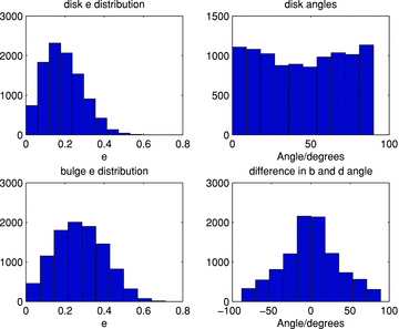
The distributions of bulge and disc ellipticities for a typical image within the fiducial set. The left-hand panels show the distribution of ellipticities for bulge and disc. The top right-hand panel shows the uniform distribution of disc position angles, and the bottom right-hand panel shows the difference between the bulge and disc positions angles.

Open in new tabDownload slide

The S/N was implemented by calculating the noise-free model flux by integrating over the galaxy model and then adding a constant Gaussian noise with a variance of unity and rescaling the galaxy model to yield the correct S/N. The S/N was scaled to match the default SExtractor (Bertin & Arnouts 1996) flux_auto–flux_err_auto parameter combination. The galaxy S/N distribution was a compact Gaussian in the majority of sets, with a variance of σ_S= 0.1, centred on (S/N)_i= 20 for the fiducial set:

(C19)

In three sets (see Section 3.1), the S/N varied for each galaxy in the set with a functional form for the S/N variation that was a Rayleigh distribution:

(C20)

where (S/N)_i= 20 and σ_S= 5.0 for these sets.

C3 The PSF models

The PSF model consisted of a static component that modelled the local PSF functional form and a spatially varying kernel that mapped the parameters of this local model across the image plane. The local functional form was a Moffat profile:

(C21)

where the scale radius r_d was a variable quantity across each image, related to the full width at half-maximum (FWHM), and the power β= 3 for all images. After generating a circular PSF, it was made into an elliptical shape by distortion using the shear matrix given in Kitching et al. (2011) such that there were three parameters which locally describe the PSF (r_d, e₁, e₂), where similarly to the galaxies the size was the pre-sheared size of the PSF.

The PSF spatial variation consisted of the following three components:

• Static component. This was spatially constant across the image and consisted of (1) a Gaussian smoothing kernel that added to the PSF size; this had a variance of 0.1 present in all images; and (2) a static additive ellipticity component of 0.05 in e_{1, PSF} and e_{2, PSF} to simulate tracking error.

• Deterministic component. This was to simulate the impact of the telescope on the PSF size and ellipticity. We used the Jarvis, Schecter & Jain (2008) model to simulate this with fiducial parameters (a₀= 0.014, a₁= 0.0005, d₀=−0.006, d₁= 0.001, c₀=−0.010), which is dominated by primary astigmatism (a₀), primary de-focus (d₀) and coma (c₀).

• Random component. To simulate the random turbulent effect of the atmosphere in some of the sets, we additionally included a random Gaussian field in the ellipticity only with a Kolmogorov power spectrum of C_ℓ=ℓ^−11/6 (see Rowe 2010; Heymans et al. 2012 for discussion on this kind of power spectrum PSF variation seen in optical weak-lensing images).

In Fig. C2 we show a typical PSF pattern for an image in a set with no random Kolmogorov variation and one in which there is a random Kolmogorov component. As described in Section 2, participants were provided with the PSF as an exact functional form, consisting of tabulated numbers for (r_d, e₁, e₂) at the position of each galaxy and as a pixelated stellar image.

Figure C2

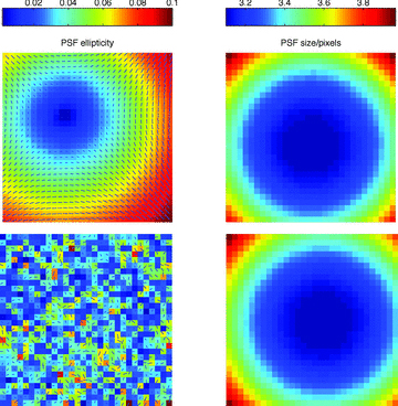
Each panel shows an entire simulated image, showing the typical PSF pattern for an image in a set (image 100 in set 1) with no random Kolmogorov component (upper panels) and for an image in a set (image 100 in set 19) with a random Kolomogorov component (lower panels). The 100 × 100 grid has been downsampled to 30 × 30 in these panels for clarity. The left-hand panels show the amplitude of the ellipticity in the colour scale, and the orientation of the PSF denoted by the whiskers. The right-hand panels show the size of the PSF in the colour scale in units of pixels. In each image in a set, these patterns changed, except in those sets where the PSF spatial variation was fixed (see Appendix D).

Open in new tabDownload slide

APPENDIX D: SET DESCRIPTION

In the table below, we provide the parameter values that define each set in the GREAT10 Galaxy Challenge simulations.

APPENDIX E: DESCRIPTION OF THE METHODS

Here we briefly summarize the methods that took part in the challenge. We encourage the reader to refer to the methods’ own papers for more details.

For each method, we show three figures. These are as follows:

• A reconstruction of the shear power spectrum for each set comparing the submitted power, true power and pixel-noise-corrected power, and the ⁠, and Q_dn values for all sets.

• The measured minus true shear on an object-by-object basis as a function of the true shear γ^t, the PSF ellipticity and size, the bulge-to-disc angle and ratio, and the bulge size; for γ^t the gradient and offset of this fit are m and c; in all cases, we make 10 bins the variable quantity. We also show a value for q, a non-linear shear response for each metric keeping m and c fixed at their best-fitting values (see equation B12).

• The m and c values as a function of PSF ellipticity and size, bulge-to-disc angle and ratio, and bulge size. In all cases, we make 10 bins the variable quantity.

Because these figures contain a wealth of information for the latter two, we plot the gradient and offset values for a linear fit through the points and display these values in the figures. In the top right-hand corner of each of the subplots, we show the difference in the reduced χ² between the best linear fit and the best constant fit (gradient equal to zero), Δχ²=χ²(gradient, offset) −χ²(offset); this can be used as an indicator of the significance of any linearly varying behaviour.

For power spectrum submissions, the latter two plots (concerned with individual one-point shear biases) will not be shown.

We have also provided postscript files of all figures in this appendix online at http://great.roe.ac.uk/data/galaxy_article_figures.

E1 ARES: Peter Melchior

Comparing the results of DEIMOS and KSB, we found several sets where the ellipticities measured with either method strongly and consistently disagreed, with relative deviations of up to 25 per cent. With additional simulations we investigated when such discrepancies between KSB and DEIMOS occur, and concluded that mainly very small, that is, badly resolved, galaxies are responsible for large relative deviations, with KSB having a too weak and DEIMOS a too strong response to galactic ellipticities. Hence, a linear combination of the shear estimates of KSB and DEIMOS appeared advantageous. With the results of our simulations, a weighting scheme was defined that aims to minimize the mean squared error on the ellipticity of each galaxy. For GREAT10, the weight for each set was adjusted independently.

E2 cat-unfold: David Kirkby, Daniel Margala

See the fit-unfold description (Appendix E4).

E3 DEIMOS: Peter Melchior, Massimo Viola, Julia Young, Kenneth Patton

DEIMOS (Melchior et al. 2011) measures the second-order moments of the light distribution using an elliptical Gaussian weight function, whose width is adjusted such as to maximize the S/N of the measurement. The centroid of the galaxy and ellipticity of the weight function are iteratively matched to the apparent (i.e. PSF-convolved) galaxy (the method has first been described by Bernstein & Jarvis 2002). The application of the weight function to the image is then corrected by considering higher order moments. These corrections become increasingly accurate with increasing width of the weight function, or the correction order. For GREAT10 we used correction of the order of 4–8, that is, considering the effect of weighting on the moments of the order of 6–10. This correction scheme has been shown to introduce very small biases of the order of 1 per cent, mostly for very small galaxies. After the deweighting, we deconvolve the galactic moments from the moments of the PSF, for which we have established an exact and analytic approach. The PSF has been measured with a weight function of the same width as the galaxy, but the ellipticity of the weight function was allowed to match the ellipticity of the PSF. From the deconvolved moments, we determine the complex ellipticity ε, which theoretically provides an unbiased estimator of the gravitational shear and thus does not need any susceptibility or responsivity corrections.

The only free parameter is the choice of the correction order, which we varied from 4 to 8 (e.g. ‘DEIMOS C6’), and the range of weight function widths. No model of either galaxy or PSF is employed. The pixel values are taken at centre-pixel positions; an interpolation to subpixel resolution is not applied.

E4 fit-unfold, cat-unfold, shapefit : David Kirkby, Daniel Margala

Each of these names refer to different submissions from the same underlying software. fit-unfold and cat-unfold were power spectrum submissions. The DeepZot analysis pipeline consists of four layers of software, implemented as c++ libraries, that were used for both the GREAT10 Galaxy Challenge and the MDM Challenge (Kitching et al., in preparation). The first layer provides a uniform interface to the GREAT10 and MDM data sets. The next layer performs PSF and galaxy shape estimation using a maximum-likelihood model-fitting method. A half-trace approximation KSB method is also implemented for comparison with earlier work and to provide a fast bootstrap of the model fit. The model-fitting code incorporates an optimized image synthesis engine and uses the MINUIT minimization library to calculate full covariance matrices. The third layer provides supervised machine learning when a suitable training set is available, and is based on the tmva package. The best results in the MDM Challenge were obtained with a 13-input neural network which derives ellipticity corrections from a combination of model-fitted parameters, covariance matrix elements, and KSB results. The final layer of the DeepZot software pipeline performs power spectrum estimation and uses the model-fitting errors to determine and subtract the variance due to shape measurement errors. The main computational bottleneck in the DeepZot pipeline is the model fit which currently requires about 500 ms per galaxy on a single Intel Xeon core for a typical fit to a 19-parameter galaxy model in which seven parameters are floating and a full covariance matrix is obtained.

E5 gfit : Marc Gentile, Frederic Courbin, Guldariya Nurbaeva

The gfit shear measurement method is a simple forward model-fitting method where the underlying galaxy is modelled using a seven-parameter Sérsic profile. The model parameters are the Sérsic index and radius (n, r_e), the galaxy two-component ellipticity (e₁, e₂), the centroid (x_c, y_c) and the flux intensity (I₀) at r= 0. The galaxy and PSF centroids were estimated using SExtractor (Bertin & Arnouts 1996).

For GREAT10, gfit used a different minimizer from that based on Levenberg–Marquardt previously used in GREAT08. The minimizer was developed at the Laboratory of Astrophysics of EPFL (LASTRO) with GREAT10 in mind. It has proven more robust and more accurate when fitting low-S/N images.

The ‘gfit den cs’ version of gfit submitted in GREAT10 involved an experimental implementation of the new DWT-Wiener wavelet-based denoising method, also developed at LASTRO. DWT-Wiener proved very successful in all other methods we submitted in the GREAT10 Galaxy Challenge (TVNN, MegaLUT). In the case of gfit, the Q factor was boosted by an estimated factor of 1.5. More details about the DWT-Wiener method can be found in Nurbaeva et al. (2011).

E6 im3shape: Sarah Bridle, Tomasz Kacprzak, Barney Rowe, Lisa Voigt, Joe Zuntz

im3shape fitted a sum of co-elliptical and co-centred Sérsic profiles. In this implementation, two Sérsic profiles were used with the Sérsic indices fixed to 1 (disc like) and 4 (bulge like) and a bulge-to-disc scale radius ratio set to 0.9. The functional form for the PSF was provided, and the convolution was performed on a grid three times the pixel resolution in each direction, with additional integration in the central pixels of the galaxy model image. The maximum-likelihood point was used, with a χ² evaluated from the full 48 × 48 postage stamp. The output ellipticity (a−b)/(a+b) was used as our shear estimate, but with a correction for noise bias for the submissions marked ‘NBC’. For the noise bias correction, a noisy simulated image was produced of a fiducial galaxy using the machinery in the im3shape code. Simulations were also produced in which the ellipticity was increased by 0.1 in one or other direction. A straight line was fitted to the output shear estimates relative to the input ellipticity to measure multiplicative and additive errors and it was verified that the multiplicative and additive errors were zero in the absence of noise. For submissions marked ‘NBC0’, two different kinds of noisy simulations were performed and used these to correct the shear estimates of the corresponding GREAT10 image sets for (i) Moffat PSF and fiducial GREAT10 S/N; and (ii) Moffat PSF and lowest GREAT10 S/N. For NBC1 the following combinations were used: (i) Moffat PSF, fiducial GREAT10 S/N, PSF FWHM 3.3 pixels, bulge scale radius 4.3 pixels; (ii) the same as the previous but PSF FWHM 3.1 pixels; (iii) the same as the previous but PSF FWHM 3.6 pixels; (iv) Moffat PSF, fiducial GREAT10 S/N, PSF FWHM 3.3 pixels, bulge scale radius 2.3 pixels; (v) the same as the previous but bulge scale radius 8 pixels; (vi) Moffat PSF, low GREAT10 S/N, PSF FWHM 3.3 pixels, bulge scale radius 4.3 pixels; (vii) the same as the previous but PSF FWHM 3.1 pixels; and (viii) the same as the previous but PSF FWHM 3.6 pixels. The optimizer used to find the location of maximum likelihood in the model parameter space was ‘PRAXIS’ (short for Principal AXIS) by Richard Brent which is available free from Netlib at http://www.netlib.org/opt/. The code is specifically written to make it easy to interchange optimizers, and alternatives are also under investigation. For more information, please refer to Zuntz et al. (in preparation) for details about the im3shape code in general and Kacprzak et al. (in preparation) for details of the noise bias calibration.

E7 KSB : Julia Young, Peter Melchior

The original KSB approach was implemented with the ‘trace-trick’, where the inversion of P^sm is achieved by replacing the entire 2 × 2 matrix with 1/2 of its trace. This approach is employed in several studies, and it has recently been shown (Viola et al. 2012) that it provides the most unbiased shear estimates for a variety of observational conditions.

To determine the galaxy centroid and the width of the circular Gaussian weight function, the same iterative method as employed in DEIMOS was used: determine the centroid such that the first moments vanish, and the size of the weight function such as to maximize S/N. For the final shear estimate, we did not apply additional fudge factors or responsivity corrections.

E8 KSB f90: Catherine Heymans

KSB f90 is a benchmark implementation of the longstanding KSB+ method (Kaiser, Squires & Broadhurst 1995; Luppino & Kaiser 1997; Hoekstra et al. 1998). This code is identical to that used in the ‘CH’ analysis of STEP1 and GREAT08 (Heymans et al. 2006; Bridle et al. 2010) and can therefore be viewed as a benchmark to compare the different simulations. KSB f90 is publicly available and can be downloaded from http://www.roe.ac.uk/~heymans/KSBf90. The code has been used to analyse the HST GEMS and STAGES surveys (Heymans et al. 2005; Heymans et al. 2008). The accuracy of KSB f90 has a strong S/N dependence as shown in this paper, yielding an incorrect redshift scaling of the lensing signal in real data. For this reason, whilst KSB f90 has been shown to perform well on average and for S/N > 20, author CH advises not to use this shape measurement method for low-S/N data.

E9 MegaLUT: Malte Tewes, Nicolas Cantale, Frederic Courbin

MegaLUT is a fast empirical method to correct ellipticity measurements of galaxies for the distortions by the PSF. It uses a straightforward classification scheme, namely a LUT, built by supervised learning. In the scope of our submissions to GREAT10, the successive steps of MegaLUT can be summarized as follows: (1) simulate a large number of realistic galaxy and PSF stamps and store the sheared galaxy ellipticities prior to the PSF convolution. This leads to a learning sample of images; (2) run a shape measurement algorithm on the galaxies and PSFs of this learning sample and create a LUT that connects the measured galaxy and PSF shapes to the known galaxy ellipticities stored in the first step; (3) for a given galaxy–PSF pair in the GREAT10 data, run the same shape measurement algorithms as in step (2). Query the LUT to identify the galaxy–PSF pairs of the learning sample that have similar measured shapes. The galaxy ellipticities of these selected pairs, as stored in step (1), yield our estimate of the galaxy ellipticity prior to the convolution by the PSF. The complex problem of PSF correction is therefore reduced to a simple and fast array indexing operation.

For the final submission ‘MegaLUTsim2.1 b20’, we denoised the galaxy and PSF images with wavelet filtering, and built simple threshold masks. The shapes were then measured using second-order moments of the masked light distributions. The LUT was generated from 2.1 million simulated galaxy–PSF pairs.

E10 method04,05,07: Micheal Hirsch, Stefan Harmeling

In a series of submissions named method0x with x∈{1, …, 7} the effect of taking higher order pixel correlations on the accuracy of shear measurement was tested. In method01, the shear was measured by subtracting the quadrupole moments of the autocorrelated images of the galaxy and corresponding PSF images. The assumption of uncorrelated noise is confirmed by the fact that the autocorrelation is highly peaked at zero shift. To get rid of this peak which impedes accurate moment estimation, a rough estimate of the noise variance was obtained by computing the variance of pixels with negative intensity values only (assuming Gaussian noise with zero mean) which was then subtracted from the central pixel. As in any other KSB-type method, noise affects moment estimation and has to be accounted for by some weighting scheme. To this end, both galaxy and star images were modulated by a Gaussian with fixed variance and zero centroid. By noticing that a pixel-wise modulation corresponds to a convolution in Fourier space, a correction for the induced error due to the modulation could be removed by subtracting the measured quadrupole moment and the fixed variance of the Gaussian distribution used for weighting in the Fourier domain. In method04, we went one step further by computing the autocorrelation of the autocorrelated galaxy or star image, otherwise pursuing the same approach as described above. By this the images are even further smoothed and are still centred such that inaccuracies in centroid estimation are not an issue in our approach. All other methods are variants of the above where the empirical moment estimation with a Gaussian weighting scheme was replaced by a model-fitting approach (method02), introduced an additional denoising step (method05), did empirical moment estimation without additional weighting (method03) and accounted for the PSF by a Wiener deconvolution of the galaxy images before moment estimation (method07).

E11 shapefit: David Kirkby, Daniel Margala

See the fit-unfold description (Appendix E4).

E12 TVNN: Guldariya Nurbaeva, Frederic Courbin, Malte Tewes, Marc Gentile

The methods NN23 func, NN19 and NN21, submitted to GREAT10, were variants of the TVNN method which is a deconvolution technique based on the combination of a Hopfield neural network (Hopfield 1982) with the Total Variation model proposed by Rudin, Osher and Faterni (Rudin 1992). In the Total Variation model, the noise in the image is assumed to follow a Gaussian distribution.

The deconvolution process is carried out by minimizing the energy function of the Hopfield Neural Network. This energy function is composed of PSF, expressed as a Toeplitz matrix, and a regularization term to minimize the noise. The latter is a Sobel high-pass operator. The deconvolution itself is done in an iterative way where at each step the neurons of the network are updated so as to minimize the energy function.

Galaxy ellipticities are then estimated from quadrupole moments computed on the 2D autocorrelation function (ACF) of the deconvolved image. The advantages of using the ACF are: (i) high-S/N shape measurement; and (ii) invariance of the ellipticity measurement with respect to data (Miralda-Escude 1991; van Waerbeke 1998)

In our submissions, the number after the acronym NN stands for the size of the input data stamps; for example, NN23 considers images with 23 pixels on a side. This is the first time full deconvolution of the data is used to carry out shape measurements.

APPENDIX F: SIMULATIONS

Inevitably, with a simulation the size of the GREAT10 Galaxy Challenge, there were several points in which the data or interpretation of the data/competition instructions was inadvertently misinterpreted by participants. The following is a list of those points:

• Approximately 1 per cent of the data were found to contain image glitches and were replaced during the challenge as a patch to the data.

• The functional PSFs used a convention in (x,y) coordinate and ellipticity for which some methods had to make the following transformations: e₂→−e₂, x→y and y→x, ⁠. This convention warning was listed in the header of every functional PSF description during the challenge.

• An additional two sets contained ‘pseudo-Airy’ PSFs using the functional form of Kuijken (2006). However, there was a misinterpretation by some participants between the functional PSF description and the PSF FITS images generated using the photon-shooting method used in the GREAT10 code. This arose because in the photon-shooting method photons at large r are generated using a uniform distribution from 0 to 1 and then their values replaced by a reciprocal; however, the PDF of such a process yields a variation of 1/r² not 1/r which when modulated by the function gives 1/r⁴ [not 1/r³, given in equation (21), Kuijken 2006; the same equation as that provided to participants]. This was identified during the challenge and all participants were informed, and the code used to produce the PSFs was made public8 on 2011 February 7 (7 months before the challenge deadline); however, we have not included the results from these sets in this paper because several submissions were affected.

Each of these issues was addressed during the challenge; however, the nature of the participation rate (see Section 5, all submissions were made in the final 3 weeks) meant that some methods did not have time to create alternative submissions before the challenge was closed officially. The challenge was extended by 1 week, into a post-challenge submission period, but those methods submitted during this time could not officially ‘win’ the competition; in the event, none of these additional submissions improved on the winning score.

When using the GREAT08/GREAT10 code we note a number of issues that should be taken into account. The S/N used in Bridle et al. (2010) is approximately half the standard definition used in this paper. Equation (A8) makes the area of the galaxy invariant under the primary ellipticity transformation (but not under the cosmological shear transformation), whereas equation (A9) does not make the PSF area invariant under the ellipticity transformation. Also the sense of the transformation in these equations of g for galaxies and e for PSFs is different; the PSF shear is in the opposite direction to the cosmic shear. Finally, we also note that there were two typos in Appendix A of Bridle et al. (2010). These were (i) in equation (A5), the top left-hand corner of the matrix should be and (ii) equation (A8) should be the transpose of what it reads.