


Abstract
The XMM Cluster Survey (XCS) is a serendipitous search for galaxy clusters using all publicly available data in the XMM–Newton Science Archive. Its main aims are to measure cosmological parameters and trace the evolution of X-ray scaling relations. In this paper we present the first data release from the XMM Cluster Survey (XCS-DR1). This consists of 503 optically confirmed, serendipitously detected, X-ray clusters. Of these clusters, 256 are new to the literature and 357 are new X-ray discoveries. We present 463 clusters with a redshift estimate (0.06 < z < 1.46), including 261 clusters with spectroscopic redshifts. The remainder have photometric redshifts. In addition, we have measured X-ray temperatures (TX) for 401 clusters (0.4 < TX < 14.7 keV). We highlight seven interesting subsamples of XCS-DR1 clusters: (i) 10 clusters at high redshift (z > 1.0, including a new spectroscopically confirmed cluster at z= 1.01); (ii) 66 clusters with high TX (>5 keV); (iii) 130 clusters/groups with low TX (<2 keV); (iv) 27 clusters with measured TX values in the Sloan Digital Sky Survey (SDSS) ‘Stripe 82’ co-add region; (v) 77 clusters with measured TX values in the Dark Energy Survey region; (vi) 40 clusters detected with sufficient counts to permit mass measurements (under the assumption of hydrostatic equilibrium); (vii) 104 clusters that can be used for applications such as the derivation of cosmological parameters and the measurement of cluster scaling relations. The X-ray analysis methodology used to construct and analyse the XCS-DR1 cluster sample has been presented in a companion paper, Lloyd-Davies et al.
1 INTRODUCTION
Clusters of galaxies provide an opportunity to explore the underlying cosmological model and the processes governing structure formation (see Voit 2005; Allen, Evrard & Mantz 2011 for reviews) and so several large-area surveys for clusters are currently underway. In this paper we present the XMM Cluster Survey (XCS), a search for serendipitous galaxy clusters in archival XMM–Newton1 (hereafter XMM) data, using the signature of X-ray extent. The original XCS concept was described in Romer et al. (2001). The main goals of the survey are to (i) measure cosmological parameters, (ii) measure the evolution of the X-ray luminosity–temperature scaling relation (hereafter LX–TX relation), (iii) study galaxy properties in clusters to high redshift, and (iv) provide the community with a high-quality, homogeneously selected, X-ray cluster sample. XCS highlights to date include the detection, and subsequent multi-wavelength follow-up, of a z= 1.46 cluster (XMMXCS J2215.9−1738; Stanford et al. 2006; Hilton et al. 2007, 2009, 2010), studies of galaxy evolution in high-redshift clusters (Collins et al. 2009; Stott et al. 2010) and forecasts of the performance of XCS for cosmological parameter estimation and cluster scaling relations (Sahlén et al. 2009, hereafter S09). In a companion paper (Lloyd-Davies et al. 2011, henceforth LD11), we describe the XCS X-ray data analysis strategy, including the XCS Automated Pipeline Algorithm (xapa). In this paper we describe the corresponding optical data analysis strategy and present the first XCS data release (hereafter XCS-DR1). A schematic of the XCS methodology is reproduced (from LD11) in Fig. 1. The components indicated with solid outlines were discussed in LD11. Those with dashed outlines are discussed herein: Redshift Follow-up (New Observations) in Section 2; Redshift Follow-up (Archive) in Section 3; Quality Control in Section 4; and Compile Cluster Catalogue in Section 5. Summaries and discussions are presented in Section 6. Brief conclusions are made in Section 7.
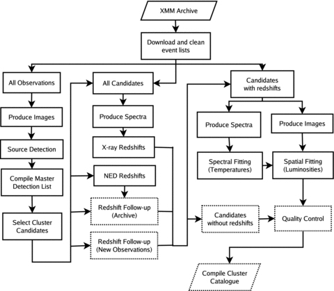
Figure taken from LD11: flowchart showing an overview of the XCS analysis methodology. This illustrates the sequence by which data from the XMM archive are used to create a catalogue of galaxy clusters. The components indicated with dashed outlines are described in this manuscript, the remainder are described in LD11.
In this paper we have relied heavily on the red-sequence, or colour–magnitude relation (CMR), technique to derive photometric redshifts using one colour (r−z) CCD imaging (Ostrander et al. 1998; Gladders & Yee 2000; López-Cruz, Barkhouse & Yee 2004). This technique takes advantage of the fact that cluster cores are populated with passively evolving elliptical galaxies that dominate the bright end of the luminosity function. The mass–metallicity relation of these ellipticals, when expressed in colour–magnitude space, has only a small intrinsic scatter (Sandage & Visvanathan 1978; Bower, Lucey & Ellis 1992; Kodama & Arimoto 1997; Stanford, Eisenhardt & Dickinson 1998; López-Cruz, Barkhouse & Yee 2004) and has become known as the E/S0 ridgeline or the cluster red-sequence. The red-sequence has been found to be remarkably homogeneous between clusters at the same redshift and has been detected to z > 1 (Lidman et al. 2008; Mei et al. 2009; Hilton et al. 2009; Papovich et al. 2010), meaning it can be used as a tool for cluster detection out to high redshifts (e.g. Gladders & Yee 2000; Gladders & Yee 2005; Muzzin et al. 2009; Wilson et al. 2009; Demarco et al. 2010; Papovich et al. 2010). The red-sequence can also be used to measure cluster redshifts because, by using appropriately placed filters, one can track the migration of the 4000 Å break feature in the spectrum of passive ellipticals. It is this redshift application that we make use of in XCS.
We note that, in the following, we have used the following terms in an XCS-specific manner; count, ObsID, candidate, candidate300 and cluster300. ‘Count’ is used as a shortening of the phrase ‘background-subtracted (0.5–2.0 keV) photon count as determined by xapa’. As explained in LD11, these count values have not been corrected for photons falling outside the xapa defined aperture (that is done during an additional spatial fitting step once the cluster redshifts are known). The count values pertain to the number of photons gathered from a single ObsID, where ‘ObsID’ is used herein to refer to each of the complex sets of XMM exposures and calibration files that comprise the 5776 XMM observations processed so far by XCS. If a candidate was detected in multiple ObsIDs, then the highest recorded count is used. ‘Candidate’ is used with reference to the LD11 definition of an XCS cluster candidate, i.e. a xapa-detected XMM source, detected with 50 or more counts, that has been classified – without warning flags – as being more extended than the instrument point spread function (PSF). Moreover, candidates must not lie in the Galactic plane or near the Magellanic Clouds. Candidates must have also passed the target filters, i.e. are genuine serendipitous detections (as far as we can tell using automated methods). To date, we have selected a total of 3675 candidates (LD11). A subset of 993, the ‘candidates300’, is of particular importance, as these were detected with 300 or more counts (see below). Similarly, ‘clusters300’ are candidates300 that have been optically confirmed as clusters.
The significance of the 300 count threshold mentioned above is twofold. First, and most importantly – because we require temperature measurements for most of our key scientific goals – we have determined (LD11) that we can derive temperatures with acceptable errors for TX > 2 keV clusters to this count limit (although we note that it is still possible to measure TX values with fewer counts, especially for cool clusters/groups, and there are many such examples in XCS-DR1). Secondly, we have demonstrated using selection function simulations (LD11) that xapa will detect most (>70 per cent) of the clusters300 that lie within the field of view of an ObsID.
Unless stated otherwise, we assume a concordance cosmology (Ωm= 0.3, ΩΛ= 0.7 and H0= 70 km s−1 Mpc−1) and error bounds are quoted by their 1σ limits. XCS-reduced X-ray images and optical images (colour-composite and grey-scale) of the XCS-DR1 clusters mentioned in the text can be viewed at http://www.xcs-home.org/datareleases (see Section 5). Full versions of the following data tables (Tables 1, 3 and A1) can be found at the same URL.
A summary of reduced observations taken by the NOAO–XMM Cluster Survey. r and z refer to exposures taken in the SDSS r- and z-band filters, respectively. A full version of this table is provided in electronic format at http://www.xcs-home.org/datareleases. These tables are ordered by increasing NXS FieldID number.
| NXS FieldID | RA (J2000) | Dec. (J2000) | No. exposures r/z | Integration time r/z (s) | Seeing r/z (arcsec) | Depth r/z (mag) | Run |
| 0002940101 | 13:07:04.7 | −23:38:51.3 | 2/3 | 1200/1500 | 1.2/1.0 | 24.1/23.4 | 4 |
| 0010620101 | 05:15:45.0 | +01:03:14.6 | 2/2 | 1200/1000 | 1.1/1.9 | 24.4/23.8 | 1 |
| 0012440301 | 22:05:04.3 | −01:54:19.1 | 2/3 | 1200/1500 | 1.4/1.4 | 24.5/23.2 | 4 |
| 0021540101 | 15:06:27.4 | +01:37:55.2 | 2/3 | 1200/1500 | 1.4/1.1 | 25.3/23.6 | 4 |
| 0025540301 | 08:38:25.5 | +25:43:40.0 | 2/3 | 1200/1500 | 2.0/1.5 | 25.0/23.7 | 3 |
| 0025541601 | 01:24:40.8 | +03:46:30.7 | 2/3 | 1200/1500 | 1.0/1.1 | 25.3/22.5 | 1 |
| 0029340101 | 06:41:43.3 | +82:14:31.4 | 2/2 | 1200/1000 | 1.0/0.9 | 25.1/23.9 | 1 |
| 0032141201 | 13:05:11.8 | −10:19:22.0 | 2/3 | 1200/1500 | 1.1/1.0 | 24.6/23.5 | 4 |
| 0037980301 | 02:25:25.7 | −03:50:59.2 | 2/3 | 1200/1500 | 1.3/1.0 | 25.6/23.0 | 5 |
| 0037981601 | 02:23:14.3 | −02:48:56.3 | 2/3 | 1200/1500 | 1.8/1.8 | 25.0/23.8 | 2 |
The XCS-DR1 Cluster Catalogue: Part I, redshifts and X-ray temperatures. A full version of this table is provided in electronic format from http://www.xcs-home.org/datareleases. Descriptions of column entries and superscripts are provided in Section 5.1.
| XCS ID | Counts | z | z-Source | TX (keV) | Alternative name | References (name, zlit) |
| (1) | (2) | (3) | (4) | (5) | (6) | (7) |
| XMMXCS J000013.9−251052.1 | 878 | 0.08 | Lit3g* | 1.8 | APMCC 948 | [1,1] |
| XMMXCS J000029.8−251211.4 | 652 | 0.15 | NXSs* | 0.81 | ||
| XMMXCS J000103.8−250353.6 | 362 | 0.91 | NXSs | |||
| XMMXCS J000141.4−154031.3 | 1135 | 0.12 | Lit3 | 1.8 | RXC J0001.6−1540 | [2,2] |
| XMMXCS J000626.2+195944.2 | 118 | 0.46 | NXSg | |||
| XMMXCS J001116.1+005211.3 | 155 | 0.36 | S82s | 0.7 | ||
| XMMXCS J001328.5−272319.0 | 484 | NXS1s | ||||
| XMMXCS J001345.2−271654.8 | 164 | NXS1s | ||||
| XMMXCS J001639.1−010211.5 | 403 | 0.17 | S82s* | 1.7 | MaxBCG J004.16184−01.03538 | [3,–] |
2 REDSHIFT FOLLOW-UP (NEW OBSERVATIONS)
We have carried out several observing campaigns in order to measure redshifts for XCS clusters. We describe our photometric follow-up in Section 2.1, the derivation of redshifts from that photometric follow-up in Section 2.2 and our spectroscopic follow-up in Section 2.3.
2.1 The NOAO-XMM Cluster Survey
The National Optical Astronomy Observatory (NOAO)–XMM Cluster Survey, or NXS, was a two-band imaging survey that gathered data across the Northern and Southern Celestial hemispheres to r≃ 24 over 38 nights. It was carried out at the NOAO 4-m facilities at Kitt Peak National Observatory (KPNO) and Cerro Tololo Inter-American Observatory (CTIO) during six observing campaigns between 2005 November and 2008 April. Slightly more time (by two nights) was allocated to the Southern hemisphere due to larger optical archival coverage in the North. During the NXS, both the KPNO and CTIO 4-m telescopes were equipped with wide-field MOSAIC CCD cameras. The KPNO MOSAIC I and CTIO MOSAIC II cameras consist of a 4 × 2 array of 2048 × 4096 pixel CCDs. These CCDs are separated by gaps of 35 pixels between columns and 50 pixels between rows. Both cameras are controlled by four Arcon CCD controllers that read out eight amplifiers for MOSAIC I (one per chip) and 16 amplifiers for MOSAIC II (two per chip). The similarity of the two MOSAIC instruments has allowed the NXS to produce a homogeneous data set across the sky. The MOSAIC I and II pixel scale of 0.26 arcsec pixel−1 and 0.27 arcsec pixel−1, respectively, provides a total imaging area of 0.36 deg2 and 0.38 deg2 on the sky. By comparison, the XMM field of view is circular with a diameter of 30 arcmin. Thus, each NXS image encompasses one XMM image. Since each ObsID typically contains multiple candidates, we opted to centre the MOSAIC camera near the aim-point of the ObsID, rather than on a specific candidate. With several thousand candidates to choose from, and only a limited number of nights at our disposal, emphasis was placed on imaging candidates300 when possible.
The primary aim of the NXS was to efficiently provide photometric redshifts for candidates to z≃ 1. Therefore, the Sloan Digital Sky Survey (SDSS;2York et al. 2000) r- and z-band filters were chosen for the survey, because these straddle the 4000 Å break over the approximate redshift range 0.3 < z < 0.6. This enhances the magnitude contrast of elliptical red-sequence galaxies detected in both bands at z≃ 0.5, and enables the estimation of red-sequence redshifts to z > 1 (Gladders & Yee 2000). MOSAIC observations were made in a typical sequence of 2 × 600 s r-band and 3 × 750 s z-band exposures. Hereafter, the set of NXS observations towards an ObsID will be referred to as an NXS field, where the NXS fieldID (see Table 1) is set to the respective ObsID name. Exposures were offset by 30 arcsec in RA and Dec. to eliminate MOSAIC chip gaps and aid the removal of cosmic rays and satellite trails in the final stacked images. If the original sequence of exposures was not taken under photometric conditions, then additional, short exposures were obtained (when possible) under photometric conditions at a later date, for calibration purposes. Over the course of the NXS project, 154 NXS fields, containing a total of 415 candidates, were observed. All of the raw data are publicly available at the NOAO Archive by searching the NOAO Portal3 (Miller, Gasson & Fuentes 2007) for the Programme ID: 2005B-0045. The total uncompressed data volume taken as part of the NXS survey is just over 500 GB. This includes 1589 science exposures and another ≃2000 calibration images. A summary of the NXS observations is presented in Table 1. Examples of NXS images of XCS-DR1 clusters are shown in Fig. 2.
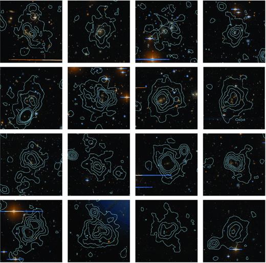
A selection of optically confirmed XCS clusters as imaged by the NOAO-XMM Cluster Survey (NXS) and classified as gold in ZooNXS. These clusters have corresponding redshifts and X-ray temperature measurements, and none of them has been previously catalogued in the literature. False colour-composite images are 3 × 3 arcmin with X-ray contours overlaid in blue. From left to right and top to bottom, the compilation displays the clusters: XMMXCS J130649.9−233128.5 at z= 0.21; XMMXCS J232221.3+193855.0 at z= 0.23; XMMXCS J205405.9−154736.5 at z= 0.27; XMMXCS J223852.3−202612.2 at z= 0.35; XMMXCS J011140.3−453908.0 at z= 0.367; XMMXCS J075427.8+220950.9 at z= 0.40; XMMXCS J232124.6+194514.8 at z= 0.40; XMMXCS J063945.9+821847.3 at z= 0.41; XMMXCS J003439.4−120715.8 at z= 0.44; XMMXCS J011624.2+325717.0 at z= 0.45; XMMXCS J092545.7+305856.9 at z= 0.52; XMMXCS J212748.7−450151.9 at z= 0.56; XMMXCS J011023.8+330544.1 at z= 0.60; XMMXCS J011632.1+330325.0 at z= 0.64; XMMXCS J100115.5+250611.5 at z= 0.763 and XMMXCS J025006.4−310400.8 at z= 0.91.
2.1.1 NXS data reduction
Images were reduced using the mscred package (Valdes 1998) written for the iraf4 environment. mscred is specifically written to reduce data taken by the NOAO MOSAIC I and MOSAIC II cameras. We briefly summarize the reduction procedures below.
After correction for cross-talk between amplifiers, and overscan trimming, the images were bias and dome flat-field corrected. Next, artefacts were corrected by generating a fringe frame and pupil-ghost frame from science images and subtracting these templates from each individual science image (MOSAIC I and II z-band images both suffer from interference fringing, and MOSAIC I z-band images also suffer from a pupil ghost). A further flat-field correction was then applied using a sky-flat. Usually, this was generated by combining suitable science images taken under similar conditions, but for the 2008 March observing campaign (due to the low number of NXS fields observed), it was necessary to make use of a sky-flat generated by the NOAO MOSAIC reduction pipeline.5 Cosmic rays, bad pixels and bleed trails were automatically identified and added to bad-pixel masks. Satellite trails were identified and masked by eye.6 An astrometric solution for each image was generated from the USNO-A2.0 catalogue using the automated task msccmatch. This solution was then used to rebin the image to a constant pixel scale to compensate for distortions across the MOSAIC field of view. The large-scale sky gradient was then removed from each image. Individual images of a particular field were then stacked by matching the background sky levels and excluding bad pixels.
Source detection and photometric measurements were performed on the stacked images using SExtractor (Bertin & Arnouts 1996) operated in dual-image mode. In this mode, source positions and apertures were identified in z-band images and then the photometry was performed in both r and z bands simultaneously to produce matched object catalogues. To facilitate dual-image mode, the r- and z-band images were registered to pixel-level accuracy to allow matched aperture photometry across both bands. To avoid introducing erroneous colour estimates in the resulting galaxy catalogues, regions near bright stars were excluded in the NXS images prior to source detection. Such regions were identified in NXS images by performing an initial run of SExtractor using a high detection threshold to locate large extended sources (>3000 connected pixels) that also contained saturated pixels. The corresponding regions were then masked in the NXS exposure maps. The final object catalogues were then produced, using a second run of SExtractor, utilizing these updated NXS exposure maps. We adopt Kron magnitudes (magauto) to estimate galaxy magnitudes and isophotal magnitudes (magiso) to calculate galaxy colours.
Photometric calibration was achieved predominantly through the use of NXS fields that happened to lie within the survey regions of the SDSS Sixth Data Release (DR6; Adelman-McCarthy et al. 2008), because SDSS sources have photometric calibration in both r and z bands accurate to within 3 per cent. Where this was not possible, observations were made of regions that contained either Southern Standard stars (Smith et al. 2002) or Landolt stars (Landolt 1992) measured in the SDSS photometric system. In addition, two NXS fields imaged during the second observing campaign were also used to calibrate subsequent runs.
For NXS fields with SDSS DR6 overlap, standard star catalogues were generated by extracting model magnitudes from the SDSS DR6 PhotoObj table for stars containing standard flags for clean photometry in the r and z bands, respectively. The positions of these SDSS stars were then cross-matched with sources in the NXS object catalogues, using 1 arcsec matching radii, to produce a matched catalogue of stars with both instrumental and corresponding standard magnitudes. Similarly, Southern Standard star positions, as well as the positions of calibrated objects in the two designated NXS calibration fields, were cross-matched with the NXS object catalogues using a 1 arcsec matching radius. In the case of Landolt stars, these were identified and photometred using the aperture photometry tool in gaia.7
Using the iraf task fitparams, the resulting catalogues of instrumental and corresponding standard magnitudes were compared in order to fit for a single zeropoint for each night, or partial night, that was deemed to be photometric. If multiple NXS fields containing calibration stars were observed over the course of a night, then the matched catalogues of instrumental and standard stars of each field were combined to fit for a single zeropoint. These updated zeropoints were then applied to the appropriate NXS object catalogues. Galactic extinction corrections were subsequently applied to NXS object magnitudes based on the dust maps and software of Schlegel, Finkbeiner & Davis (1998).
Star–galaxy separation was determined for each NXS image using the method presented in Metcalfe et al. (1991), based on identifying the locus of stars in the concentration–magnitude plane. A concentration parameter was computed using aperture magnitudes measured within four and 12 pixels (≃1 and ≃3 arcsec) in diameter. Star–galaxy separation was performed in the r band and results in a clear separation of stars from galaxies at magnitudes typically brighter than r≃ 22. At fainter magnitudes, we classified all objects to be galaxies, regardless of their concentration parameter.
The 90 NXS fields taken under photometric conditions have a typical seeing of 1.39 and 1.23 arcsec in the r and z bands, respectively. For an additional 11 NXS fields, it was possible to calibrate them a posteriori using short integrations taken on subsequent photometric nights. Observations of another 30 NXS fields were taken under non-photometric conditions, but the images were still of sufficient quality that they could be used for the optical identification work described in Section 4.1. The mean depth of the calibrated NXS fields, as given by the 5σ point source detection limit, are r= 25.0 and z= 23.8. Based on the Bruzual & Charlot (2003) population synthesis models and the assumption that the bulk of the signal in detecting a cluster comes from the galaxies brighter than about 0.5 mag below L★ (Gladders & Yee 2000), these limits should be sufficient to detect clusters, and measure CMR redshifts, to z≃ 1. In total, 366 candidates are contained within photometrically calibrated NXS fields.
2.2 Photometric redshifts
We have applied the CMR-redshift technique to single-colour (r−z) photometric images of candidates. The photometry has come either from the NXS project (Section 2.1) or from the SDSS (Section 3.1). Our redshift algorithm is based on that presented in Gladders & Yee (2000), in that it identifies overdensities of galaxies exhibiting a red-sequence and assigns a redshift based on the red-sequence colour. However, it differs from Gladders & Yee (2000) in that it assumes the cluster centre is defined by the X-ray centroid of the corresponding XCS candidate (rather than by the centroid of a galaxy overdensity).
For each candidate, potential cluster galaxies are extracted from a circular region with a radius set to twice its X-ray extent, as measured by the xapa algorithm. The colour distribution of these galaxies is then compared to that of an assumed field galaxy sample (normalized to the cluster area) to identify potential overdensities of red-sequence galaxies. For NXS, the field galaxy sample was generated separately for each NXS field. To minimize contamination of the field sample (by galaxies that reside within clusters), galaxies were masked from the field sample if they fell in areas that overlapped with XCS candidates (as mentioned previously, a given NXS field will typically cover multiple candidates). The masking radius was fixed at 0°.15 for each of the candidates, because we do not know a priori the redshift or temperature of their associated clusters, and so cannot use physical radii, such as R200. We note that in all cases, the 0°.15 masking radius was larger than the galaxy extraction radius – so the contamination, by cluster galaxies, of the field sample should be low.
 is the negative log likelihood; z is the cluster redshift; b(z) is the background distribution, given by the colour distribution of the local field sample; ΛN is a measure of cluster richness and corresponds to the total number of cluster galaxies above the background distribution; M(z) is our red-sequence cluster model and D is the total number of galaxies within twice the X-ray extent. The red-sequence cluster model we adopt is a Gaussian distribution in colour (Koester et al. 2007b):
The maximum ridgeline likelihood is found by considering a grid of red-sequence colours at redshifts 0.1 ≤z≤ 1.0 and richness 0 ≤ΛN≤ 50 in discrete steps of Δz= 0.01 and ΔΛN= 1, respectively. Each model redshift is converted into a red-sequence colour using a theoretical map of red-sequence colour relations with redshift. This map is based on the slope of the composite red-sequence of 73 clusters at z≃ 0.1 detected by the SDSS-C4 survey (Miller et al. 2005), which is then evolved with redshift using the Bruzual & Charlot (2003) population synthesis models assuming a single-burst Salpeter initial mass function (IMF) with a formation redshift of zf= 2.5 (Gladders & Yee 2005).
An estimate of the cluster richness (ΛN) is produced with the estimate of the cluster redshift (equation 1). The meaning of ΛN is specific to the particular method used. In this case, it refers to the number of background-subtracted, red-sequence galaxies extracted from a circular region with a radius set to twice the X-ray extent, as measured by the xapa algorithm. We note that the ΛN value can be considered to be a lower limit to the true richness of the cluster. This is because the adopted extraction radius is typically less than R200 (an approximation to the virial radius, defined as the radius at which the overdensity has fallen to 200 times that of the critical density). Moreover, the entire R200 region is not always contained within an NXS field (the fields are centred on the ObsID aim-point rather than on a specific candidate).
The best-fitting redshift, or CMR redshift, will have an associated error that depends on a range of factors including the true redshift, the sensitivity of the image, the accuracy of the photometric calibration, the quality of the local field sample and the appropriateness of the red-sequence model. The error on an individual CMR redshift can only be determined once spectroscopic follow-up has taken place, but the typical error on a CMR redshift can be externally determined via comparisons with measured spectroscopic redshifts (see Section 5.3). That said, we do calculate χ2 error estimates for the individual redshift measurements and these χ2 errors are used as an indication of the quality of the individual fits.
We deemed a CMR redshift fit to be unreliable if the χ2 error was too high (σz > 0.1), or if the richness was too low (ΛN < 5; see below), or if the NXS images were taken under non-photometric conditions. Excluding these unreliable fits, a total of 224 CMR-redshift measurements were made using NXS data. We note that the drop in number from the 366 candidates contained within photometrically calibrated NXS fields (see above) to the 224 with reliable CMR redshifts is primarily due to the ΛN < 5 cut. We assess the accuracy of NXS CMR redshifts in Section 5.3.
The choice of ΛN > 5 for the richness cut was chosen after testing a range of values and after consultation with the literature (e.g. Geach, Murphy & Bower 2011, also uses a cut-off of five galaxies). We note that applying this cut does not preclude the inclusion of distant clusters in XCS-DR1, just their associated estimated redshift: of the 197 cluster candidates with ΛN < 5 values, 11 (i.e. ≃ 5 per cent) were optically confirmed as clusters via visual inspection (using ZooNXS, see Section 4.1) and included in XCS-DR1.
2.3 Spectroscopic redshifts
Table 2 lists the mean spectroscopic cluster redshifts obtained by members of the XCS team for 35 candidates. Of the objects in the table, only the spectroscopic redshift of XMMXCS J2215.9−1738 (z= 1.46) has previously been published (Stanford et al. 2006; Hilton et al. 2007, 2009, 2010). At the start of our spectroscopic programme, candidates were selected for follow-up either to fill RA gaps during the follow-up of the SDSS-II Supernova Survey (Östman et al. 2011; Frieman et al. 2008) or because they were judged by eye to be potential z > 1 clusters (and hence suitable for Keck or Gemini follow-up). However, as the project matured, the target selection was informed by X-ray redshift estimates (see LD11), thus allowing us to design a follow-up programme that both sampled the LX–TX(z) relation, and allowed us to determine the accuracy of the CMR redshifts (Section 5.3).
Spectroscopic redshifts for XCS-DR1 clusters acquired by XCS team members (many more spectroscopic cluster redshifts are included in XCS-DR1, but those were obtained from archives or from the literature). The N(z) column lists the number of concordant redshifts obtained for each cluster. For clusters with only one spectroscopic redshift, the z column gives the redshift of the suspected BCG; otherwise the z column gives the mean galaxy redshift. The rightmost column lists the date(s) of observation, the observing programme number (for ESO or Gemini) or references, as appropriate. Uncertainties on the spectroscopic redshift values are not presented but are assumed to be at the level of the cluster velocity dispersion, i.e. σv < 2000 km s−1.
| XCS ID | z | N(z) | Telescope/instrument | Comments |
| XMMXCS J003548.2−432232.4 | 0.633 | 12 | GMOS/Gemini | GS2010B-Q-46 |
| XMMXCS J011140.3−453908.0 | 0.367 | 11 | NTT/EFOSC2 | 2008 Jul 28, 30-31 (Programme ID: 081.A-0843(A)) |
| XMMXCS J012400.0+035110.8 | 0.883 | 7 | Keck/DEIMOS | 2006 Sept 21 |
| XMMXCS J015241.1−133855.9 | 0.825 | 10 | Keck/DEIMOS | 2005 Sept 2, 2006 Sept 21 |
| XMMXCS J023346.0−085048.5 | 0.25 | 1 | NTT/EMMI | 2006 Sept 15 (Programme ID: 077.A-0437(A)) |
| XMMXCS J025006.4−310400.8 | 0.908 | 6 | Gemini/GMOS | GS2010B-Q-46 |
| XMMXCS J030145.5+000335.8 | 0.694 | 3 | Gemini/GMOS | GS-2010B-Q-46 |
| XMMXCS J030317.4+001238.4 | 0.594 | 1 | NTT/EMMI | 2006 Sept 15 (Programme ID: 077.A-0437(A)) |
| XMMXCS J032553.3−061719.9 | 0.322 | 2 | NTT/EMMI | 2007 Dec 9 (Programme ID: 080.A-0024(C)) |
| XMMXCS J035417.0−001006.6 | 0.214 | 2 | NTT/EMMI | 2007 Dec 9 (Programme ID: 080.A-0024(C)) |
| XMMXCS J041944.6+143904.5 | 0.193 | 2 | NTT/EMMI | 2006 Oct 17 (Programme ID: 078.A-0325(C)) |
| XMMXCS J045506.3−532343.8 | 0.410 | 1 | NTT/EMMI | 2006 Dec 13 (Programme ID: 078.A-0325(A)) |
| XMMXCS J051610.0+010954.0 | 0.318 | 2 | NTT/EMMI | 2007 Dec 7 (Programme ID: 080.A-0024(C)) |
| XMMXCS J080612.6+152309.0 | 0.41 | 1 | WHT/ISIS | 2007 Dec 1–3 (Programme ID: P53) |
| XMMXCS J091821.9+211446.0 | 1.007 | 16 | Gemini/GMOS | GN-2010B-Q-65 |
| XMMXCS J095105.7+391742.9 | 0.47 | 1 | WHT/ISIS | 2007 Dec 1–3 (Programme ID: P53) |
| XMMXCS J095940.8+023111.3 | 0.720 | 14 | Gemini/GMOS | GS2010B-Q-46 |
| XMMXCS J100115.3+250612.4 | 0.763 | 12 | Gemini/GMOS | GN-2010B-Q-65 |
| XMMXCS J100201.7+021332.8 | 0.832 | 6 | Gemini/GMOS | GS2009B-Q-80 |
| XMMXCS J102136.9+125643.2 | 0.325 | 1 | NTT/EMMI | 2006 Dec 14 (Programme ID: 078.A-0325(C)) |
| XMMXCS J104422.2+213025.2 | 0.515 | 7 | Gemini/GMOS | GN-2010B-Q-65 |
| XMMXCS J105040.6+573741.4 | 0.689 | 12 | Gemini/GMOS | GN-2010B-Q-65 |
| XMMXCS J111645.5+180047.7 | 0.662 | 7 | Gemini/GMOS | GN2005B-Q-56 |
| XMMXCS J111726.0+074327.7 | 0.482 | 15 | Gemini/GMOS | GS2010B-Q-46 |
| XMMXCS J112349.3+052956.8 | 0.652 | 11 | Gemini/GMOS | GS-2010B-Q-46 |
| XMMXCS J130601.4+180145.9 | 0.927 | 3 | Keck/LRIS | 2005 Feb 10 |
| XMMXCS J150652.9+014424.8 | 0.653 | 2 | NTT/EFOSC2 | 2008 Jul 29 (Programme ID: 081.A-0843(A)) |
| XMMXCS J153643.9−141024.2 | 0.40 | 2 | NTT/EFOSC2 | 2008 Jul 30 (Programme ID: 081.A-0843(A)) |
| XMMXCS J200703.1−443757.6 | 0.202 | 1 | NTT/EFOSC2 | 2008 Jul 31 (Programme ID: 081.A-0843(A)) |
| XMMXCS J204134.7−350901.2 | 0.425 | 1 | NTT/EFOSC2 | 2008 Jul 30 (Programme ID: 081.A-0843(A)) |
| XMMXCS J212807.6−445417.3 | 0.538 | 4 | NTT/EFOSC2 | 2008 Jul 27–28, 30–31 (Programme ID: 081.A-0843(A)) |
| XMMXCS J215221.0−273022.6 | 0.826 | 9 | Gemini/GMOS | GS-2010B-Q-46 |
| XMMXCS J221559.6−173816.2 | 1.457 | 31 | Various | See Stanford et al. (2006); Hilton et al. (2007, 2009, 2010) |
| XMMXCS J231852.3−423147.6 | 0.114 | 1 | NTT/EMMI | 2007 Dec 10 (Programme ID: 080.A-0024(C)) |
| XMMXCS J235708.6−241449.2 | 0.588 | 10 | NTT/EFOSC2 | 2008 Jul 27, 29–31, Aug 1 (Programme ID: 081.A-0843(A)) |
The spectroscopic observations were performed over several years at a number of different observatories with a variety of instruments, as summarized in Table 2. Data taken with the DEep Imaging and Multi-Object Spectrograph (DEIMOS; Faber et al. 2003) at the Keck observatory were processed with version 1.1.4 of spec2d, the pipeline developed for the DEEP2 galaxy redshift survey (Davis et al. 2003). All Gemini Multi-Object Spectrograph (GMOS; Hook et al. 2003) observations were obtained in nod-and-shuffle mode, and reduced in a manner similar to that described in Hilton et al. (2010). An example of a cluster that was spectroscopically confirmed in one of the GMOS observing programmes is shown in Fig. 3. The ESO (European Southern Observatory) Multi-Mode Instrument (EMMI; Dekker, Delabre & Dodorico 1986) and ESO Faint Object Spectrograph and Camera (EFOSC2; Buzzoni et al. 1984; Snodgrass et al. 2008) at the New Technology Telescope (NTT) were used to obtain long-slit spectroscopy of likely (as judged by eye) Brightest Cluster Galaxies (BCGs). Multi-object spectroscopic observations were also obtained for some clusters using EFOSC2. All of the data obtained at ESO were reduced using iraf in the standard manner.
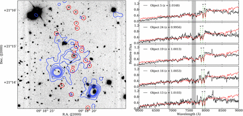
The z= 1.01 cluster XMMXCS J091821.9+211446.0. The left-hand panel shows a 3 × 3 arcmin Gemini GMOS i-band image, with X-ray contours overlaid (blue) and spectroscopically identified cluster members circled in red. The right-hand panel shows the GMOS spectra (black lines; not flux calibrated) of a selection of members highlighted in the image. A redshifted LRG spectral template (red line) is shown for each galaxy.
Redshifts were measured either from visually identified spectral features or using the cross-correlation method implemented in the rvsao iraf package (Kurtz & Mink 1998). Table 2 lists the number of secure concordant redshifts obtained for each cluster. Several of the clusters listed in Table 2 have only one redshift measurement; in these cases, the quoted redshift is that of the likely BCG. Redshifts, and coordinates, of individual galaxies used to determine cluster redshifts in Table 2 can be found as follows: for XMMXCS J221559.6−173816.2, see Stanford et al. (2006); Hilton et al. (2007, 2009, 2010); for clusters targeted during Gemini/GMOS campaigns, see Hilton et al. (in preparation); and, for the other clusters, see Table A1.
We highlight here two clusters from Table 2. First, a new (to the literature) z > 1 cluster, optically confirmed in the NXS (Section 2.1), with multi-object spectroscopic confirmation (XMMXCS J091821.9+211446.0, z= 1.01, Fig. 3). Second, a new (to the literature) cluster, XMMXCS J015241.1−133855.9 at z= 0.83, within a projected distance of ≃8.7 Mpc from the well-studied merger system XMMXCS J015242.2−135746.8 (or WARP J0152.7−1357, Ebeling et al. 2000; Romer et al. 2000; Demarco et al. 2005; Girardi et al. 2005; Maughan et al. 2006).
3 REDSHIFT FOLLOW-UP (ARCHIVE)
In addition to our own redshift follow-up work, we have been able to extract a large number of redshifts (both spectroscopic and photometric) for our candidates using data archives and from the literature. We describe the extraction of redshifts from the SDSS Seventh Data Release (DR7; Abazajian et al. 2009) in Sections 3.1 (photometric) and 3.2 (spectroscopic), and the extraction of redshifts from the literature in Section 3.3. We note that no XCS-determined X-ray redshifts are included in XCS-DR1. These redshifts have been shown to be reliable (at the Δz < 0.1 level) in 75 per cent of cases (LD11) and so, in principle, we could have used them for XCS-DR1. However, in practice, there were only 42 overlaps between the sample of candidates with reliable X-ray redshifts and the XCS-DR1 list, and all of these have other redshift determinations of higher quality.
3.1 Redshifts from SDSS (photometric)
The red-sequence redshift algorithm described above (Section 2.2) was also applied to each of the candidates that fall in the SDSS DR7 footprint.8 Included in SDSS DR7 is a 270 deg2 co-added stripe, known as Stripe 82, and referred to as S82 hereafter, that reaches a depth ≃2 mag fainter than the regular survey. We have used both data sets to determine CMR redshifts from SDSS DR7. At the time of writing (2011 June), 1721 candidates lie within the SDSS DR7 footprint, of which 69 lie within the S82 footprint.
Galaxy samples were extracted from the Galaxy View, which contains photometric information for all primary objects imaged by SDSS and subsequently classified as galaxies. We use the SDSS measurement ModelMag to provide galaxy magnitudes and calculate colours for each galaxy, and apply the Galactic extinction corrections supplied by the SDSS based on the dust maps by Schlegel et al. (1998). We specify that all galaxies must contain the standard flags for clean photometry in both the r and z bands. In this manner, potential cluster galaxy samples were generated for each candidate by retrieving de-reddened model r and z magnitudes for all SDSS DR7 and S82 galaxies falling within an extraction radius of twice the xapa extent.
As the SDSS is a large, homogeneous survey, a universal field sample could be constructed (rather than the field-by-field approach adopted for NXS; Section 2.2). For this, a random sample of 50 (20) ObsIDs within the SDSS DR7 (S82) footprint was selected as the basis for a field sample. ObsIDs with incomplete SDSS coverage, or those containing image defects or saturated objects, were not used. De-reddened model r- and z-band magnitudes were retrieved for all galaxies with clean photometry across the regions covered by each of the 50 (20) ObsIDs.
To minimize contamination of the field sample (by galaxies that reside within clusters), galaxies were masked from the field sample if they fell in areas that overlapped either with XCS candidates or with known clusters [identified using NASA/IPAC Extragalactic Database (NED)]. In the case of NED clusters, the redshifts are usually known, but the temperatures typically are not. So, to be conservative, we used an R200 radius for the masking that assumes a cluster temperature of TX= 4 keV (less than 30 per cent of XCS clusters are hotter than this, i.e. would have larger R200 values; see Fig. 13). The R200 values were calculated according to the method outlined in section 3.2 of S09. In the case of XCS candidates, we do not a priori know their redshift or temperature, so we chose a fixed masking radius of 0°.15 (as was the case for NXS, see Section 2.2). This process yielded a single combined field sample containing 52 660 (207 693) galaxies covering a combined total area of 18.10 deg2 (5.87 deg2) derived from SDSS DR7 (S82).
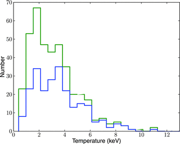
The temperature distribution for the 401 clusters with measured X-ray temperatures in XCS-DR1. The green line represents the total sample, while the blue line represents clusters300.
Similar to the approach taken with NXS CMR redshifts (Section 2.2), we deemed a SDSS DR7 (S82) CMR-redshift fit to be unreliable if the χ2 error was too high (σz > 0.1), or if the richness was too low (ΛN < 5). After excluding these unreliable fits, and candidates with less than 100 counts (DR7 only; see Section 4.1), a total of 574 and 51 CMR-redshift measurements were made using DR7 and S82 data, respectively. We assess the accuracy of DR7 and S82 CMR redshifts in Section 5.3.
3.2 Redshifts from SDSS (spectroscopic)
Luminous Red Galaxies, or LRGs, have been targeted by SDSS for spectroscopic follow-up using colour and magnitude cuts designed to select luminous (L > 3L*), intrinsically red, elliptical galaxies (Eisenstein et al. 2001). As LRGs predominantly reside in the central regions of dense cluster environments, we can make the assumption that an identified LRG coincident with an X-ray emitting cluster is part of that cluster. The spectroscopic redshift of this LRG (or group of LRGs) can then be adopted as the cluster redshift.
Because the 4000 Å break migrates with redshift, two colour cuts are necessary to select LRGs within SDSS imaging: we use the low-redshift (z < 0.45) colour cuts of Eisenstein et al. (2001) and the high-redshift (0.45 < z < 0.7) cuts of Padmanabhan et al. (2005) and Collister et al. (2007). From the resulting combined sample, an LRG (and its spectroscopic redshift) is assigned to an XCS candidate if it lies within 175 kpc of the X-ray centroid (assuming the redshift of the LRG). This matching radius was chosen because it was both free from high levels of contamination (the ratio of real-to-false matches was found to be 18 per cent when comparing the assigned LRG redshift to corresponding cluster redshifts in the 400d catalogue; Burenin et al. 2007) and consistent with the results from Lin & Mohr (2004) (who found that 70 per cent of BCGs are located within 5 per cent of the cluster virial radius, R200, from the X-ray centroid). There are instances, however, where multiple LRGs are assigned to a given XCS candidate. Some of these will be groups of LRGs belonging to the same cluster halo. These are identified by scanning in redshift intervals of Δz= 0.05 and counting the number of (assumed) Gaussian colour error distributions overlapping in segments of Δz= 0.1. A cluster redshift is then assigned from a given group of LRGs using the following hierarchy: if one distinct group of LRGs is found, then the weighted mean redshift and weighted error of that group are assigned to the XCS candidate; if more than one group of LRGs is found, the group with the larger number of LRGs is chosen; if the number of LRGs within two groups is identical, then the group with the redshift closest to the CMR redshift determined from the deepest imaging data (Sections 2.2 and 3.1) is chosen.
It was found, using eye-ball inspection, that when low-redshift (z < 0.08) LRGs were associated with XCS candidates, the matches were typically erroneous. This is because the 175 kpc search radius subtends a large angle on the sky at low LRG redshifts. Therefore, only LRG redshifts at z≥ 0.08 were typically used for XCS-DR1. However, we did make exceptions if the candidate had a measured CMR redshift pegged at the algorithm’s minimum value (z= 0.1). In this instance, the candidate was judged to be at low redshift and so could be safely associated with LRG redshifts below z= 0.08. There are five such cases in XCS-DR1: XMMXCS J010720.2+141604.2; XMMXCS J015315.0+010214.2; XMMXCS J115112.0+550655.5; XMMXCS J134326.9+554648.3 and XMMXCS J163015.6+243423.2. In summary, 265 candidates were associated with spectroscopic derived from SDSS LRGs.
3.3 Redshifts from the literature
All candidates have been cross matched using a simple automated NED query to determine whether they have been catalogued by an earlier cluster survey (Section 5). In addition, a more complex NED query has been used to determine which of the candidates can be associated with a published redshift. This search involves an iterative analysis of the XMM data, and the technical aspects have been described in LD11. To date 493 literature redshifts, or zlits, have been extracted from NED using this process. The automated nature of the zlit collection means that not all of the extracted redshifts are correct. Therefore, for XCS-DR1 we have taken a conservative approach of only using literature redshifts if zlit≥ 0.08. After applying this cut,9 345 zlit values remain. To these, we have added by hand 11 redshifts that were not in NED at the time when the automated zlit extraction was performed [four of these 11 redshifts were taken from a recent data release by the XMM-Large-Scale Structure (XMM-LSS) survey by Adami et al. (2011), three redshifts were taken from a parallel study, Harrison et al. (2012) (hereafter H12; see Section 5.2), two redshifts were taken from Šuhada et al. (2011), a single redshift was taken from Lamer et al. (2008), and a single redshift was taken from Boehringer et al. (2005)]. In addition, we updated eight of the default NED redshifts with improved values available in the literature [six redshifts from Adami et al. (2011) for XMM-LSS clusters, a single redshift from Hashimoto et al. (2005) (for RX J105346.6+573517), and a single redshift from Stanford et al. (2006) (for XMMXCS J2215.9−1738; see Table 2)].
The NED-based zlit collection method cannot discern automatically whether individual redshifts were spectroscopic or photometric. However, this information is important to XCS, both to assess the reliability of derived quantities (especially X-ray luminosities) and to determine the typical error on XCS photometric redshifts (Section 5.3). Therefore, we have made a manual check of the respective publication(s) for each of the 229 XCS-DR1 clusters with associated zlit values (210 coming from the automatic NED search, the remainder coming from the sources described above). We encourage the reader to revisit these publications if more information is required about a particular zlit value, e.g. individual member galaxy redshifts and coordinates.
4 QUALITY CONTROL
A quality control step is necessary for XCS-DR1 because candidates are selected in a fully automated fashion (Fig. 1). Whilst automation is important to XCS – for both efficiency and to maintain statistical robustness – it can result in contamination of the candidate list by: (i) extended non-cluster X-ray sources (e.g. low-redshift galaxies); (ii) non-extended X-ray sources (e.g. blended point sources) and (iii) clusters that were the intended target of the respective ObsID (or physically associated with it). Therefore, some quality control must be applied before releasing a confirmed cluster catalogue based on a given input candidate list. This has been carried out for XCS-DR1 using one or more of the following: an XCS-Zoo (Section 4.1); information from the literature (Section 4.2); our own spectroscopy (Section 4.2) and checks of the ObsID headers (Section 4.3).
4.1 Candidate identification using XCS-Zoo
Both the name and the methodology of XCS-Zoo were inspired by the SDSS Galaxy Zoo project (Lintott et al. 2008). The Galaxy Zoo project took advantage of community input to morphologically classify SDSS galaxies over the web. The XCS-Zoo project is similar, in that it draws on a team of volunteers – either members of XCS or astronomers at affiliated universities – to classify XCS cluster candidates, and this classification is done using eye-ball inspection via a web interface. However, XCS-Zoo is on a much smaller scale than Galaxy Zoo. Moreover, unlike the hundreds of thousands of Galaxy Zoo volunteers, all 23 XCS-Zoo participants are co-authors of this paper.
The XCS-Zoo allowed us to establish, by consensus, whether a candidate had an obvious optical cluster counterpart. Candidates were included in XCS-Zoo if optical10 CCD imaging was available from the NXS (Section 2.1) or SDSS DR7 (both the regular survey and S82). A separate XCS-Zoo was undertaken for each of the three imaging surveys, and hereafter we refer to these as ZooNXS, ZooDR7 and ZooS82, respectively. Each candidate was classified at least five times per Zoo, even if they were covered by multiple imaging surveys. The number of candidates that could potentially have been classified by ZooDR7 was much larger (1721) than the other two Zoos (484 in total), and so we set a minimum X-ray count (>100) threshold for ZooDR7. This reduced the number of candidates included in ZooDR7 to a more manageable 1151.
The inspected candidates were classified into one of the following categories of cluster: gold; silver and bronze. A fourth category (other) was used for any remaining candidates (Section 4.1.1). The XCS-Zoo categorization of each source was based upon the following information: a series of X-ray image cutouts (3 × 3, 6 × 6, 12 × 12 arcmin), highlighting X-ray contours and the region enclosed by the xapa X-ray extent; a corresponding series of colour-composite optical images (with and without X-ray contours overdrawn) and an image highlighting the location of the candidate within the ObsID.
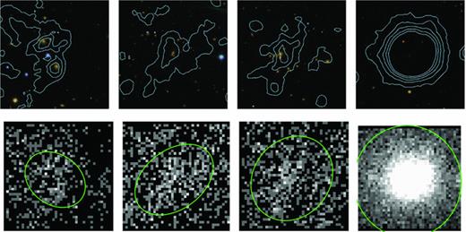
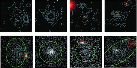
To be assigned a classification of gold, a candidate must have an unambiguous overdensity of galaxies coincident (i.e. within the extent of the xapa defined source ellipse) with an unambiguous11 extended X-ray source (Fig. 4). Candidates classified as silver must have either an unambiguous overdensity of galaxies associated with an acceptable extended X-ray source, or an unambiguous extended X-ray source associated with a suspected galaxy overdensity and/or BCG (Fig. 5). Candidates classified as bronze were judged likely to be clusters, but could not be confirmed as such using only the information available in XCS-Zoo (Fig. 6).
The first four clusters presented in the electronic version of Table 3 classified as gold in ZooDR7 (Section 4.1). False colour-composite images are 3 × 3 arcmin with X-ray contours overlaid in blue. Corresponding X-ray images are shown below each optical image (lighter regions show areas of increased X-ray flux). The shape of the xapa-detected extended (point) source ellipses are highlighted in green (red). From left to right, the clusters are: XMMXCS J001737.4−005235.4 at z= 0.21; XMMXCS J010858.7+132557.7 at z= 0.15; XMMXCS J083454.8+553420.9 at z= 0.24; and XMMXCS J092018.9+370617.7 at z= 0.21.
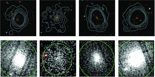
Four XCS-DR1 clusters that have been classified as silver in ZooDR7 (Section 4.1). False colour-composite images are 3 × 3 arcmin with X-ray contours overlaid in blue. Corresponding X-ray images are shown below each optical image (lighter regions show areas of increased X-ray flux). The shape of the xapa-detected extended source ellipses are highlighted in green. The right-most cluster is an example where the classification (as silver) was based predominantly on the X-ray data, the other three are examples where the classification (as silver) was based predominantly on the galaxy overdensity (these three represent the first silver entries in the electronic version of Table 3). From left to right, the clusters are: XMMXCS J004231.6+005119.9 at z= 0.15; XMMXCS J004252.6+004303.1 at z= 0.27; XMMXCS J004333.7+010109.6 at z= 0.20 and XMMXCS J122658.1+333250.9 at z= 0.89.
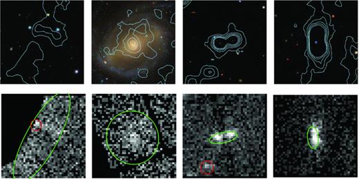
The first four clusters in the electronic version of Table 3 classified as bronze in ZooDR7 (Section 4.1), all four have been optically confirmed using information in the literature (Section 4.2). False colour-composite images are 3 × 3 arcmin with X-ray contours overlaid in blue. Corresponding X-ray images are shown below each optical image (lighter regions show areas of increased X-ray flux). The shape of the xapa-detected extended (point) source ellipses is highlighted in green (red). From left to right, the clusters are: XMMXCS J092111.0+302758.2 at z= 0.43; XMMXCS J095951.4+014052.1 at z= 0.37; XMMXCS J101056.3+555711.5 at z= 0.17 and XMMXCS J103100.1+305134.9 at z= 0.14.
Each category was allocated an integer (from 1 to 4), with 4 for gold through to 1 for other. The average value (after rounding down) was adopted for a particular candidate, based on the five (or more) classifications available per XCS-Zoo. If a candidate was included in more than one XCS-Zoo, and had gained different average categorizations, then the category with the highest numerical score was adopted.
Excluding duplicates, the number of candidates classified as gold, silver, bronze and other via XCS-Zoo was 82, 311, 329 and 766, respectively. Including duplicates, 415, 1151 and 69 candidates were classified by ZooNXS, ZooDR7 and ZooS82, respectively. For the purposes of XCS-DR1, we have decided to include all candidates with gold and silver classifications, because we judge those to have been confirmed as clusters. By contrast, only a subset of those with bronze classifications are included in XCS-DR1 because, based on XCS-Zoo alone, we cannot be sure they are clusters (even if they have measured CMR redshifts). Therefore, only the 18 bronze candidates that have been confirmed as being clusters by some other (to XCS-Zoo) method are included (Section 4.2). Once deeper optical imaging, and/or multi-object spectroscopy, is available, we expect that many of the 329 candidates in the bronze category will be confirmed as clusters. This has already been demonstrated in 17 cases where candidates that were categorized as bronze in ZooDR7 were silver or gold in the ZooNXS or ZooS82 (Fig. 8). In summary, excluding duplicates, 81, 307 and 18 candidates12 classified as gold, silver and bronze (and none of those classified as other, Section 4.1.1) appear in XCS-DR1 as confirmed clusters.
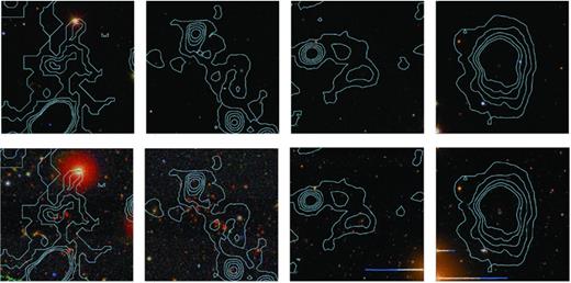
Four examples of XCS-DR1 clusters classified as bronze in ZooDR7 (Section 4.1) that were subsequently classified as gold or silver in ZooNXS or ZooS82. False colour-composite images are 3 × 3 arcmin with X-ray contours overlaid in blue. Images from SDSS DR7 are shown above the corresponding deeper image (Stripe 82 on far- and mid-left, NXS on far- and mid-right). From left to right the clusters are: XMMXCS J030205.1−000003.6 at z= 0.65; XMMXCS J030317.4+001238.4 at z= 0.59; XMMXCS J083115.0+523453.9 at z= 0.52 and XMMXCS J083025.9+524128.4 at z= 0.99.
In principle, we would like to include all the remaining clusters that fall within the NXS, DR7 and S82 footprints in future data releases. These comprise 311 bronze clusters and 766 other objects. In practice, this is too many to follow-up individually, so we have decided to concentrate our efforts on the candidates300. Applying the count threshold reduces the numbers of candidates requiring follow-up by roughly two thirds. Moreover, we have found (see Section 4.1.1) that 75 per cent of the other candidates300 do not require additional follow-up, but can rather be removed immediately (as contaminants) without impacting the completeness of a final cluster catalogue. Thus only 43 other, in addition to the 95 bronze, candidates300 require additional follow-up. This process has recently begun based on imaging campaigns at the William Herschel Telescope (WHT).13 The identities, and redshifts, of the candidates with fewer counts are likely to remain unknown until more sensitive large-area imaging surveys are publicly available [e.g. from the Dark Energy Survey (DES), Large Synoptic Survey Telescope (LSST) or Pan-Starrs4].14
4.1.1 Candidates not classified as clusters
The XCS-Zoo exercise was primarily designed to pick out the obvious clusters in the candidate list; these clusters can be used in the short term for a variety of scientific applications (Section 6.5) and in the longer term can be used to inform improvements to both the optical and X-ray methodology used by XCS. Therefore, anything that was not obviously a cluster ended up in the other category. On the completion of XCS-Zoo, we reviewed all the candidates300 in the other category and found they could be sub-divided into the following classes:
Masking or reduction issues (≃50 per cent): before running the xapa software on a given ObsID, the XCS generated image is examined by eye. Any sub-regions unsuitable for cluster searching are saved into a mask file, and some files are removed from the pipeline entirely. The removed files include those with atypically high backgrounds (this can occur if one of the XMM cameras was behaving abnormally during the exposure). The masked regions include those covered by large extended objects, such as low-redshift clusters, or those with out-of-time bleed trails (see LD11). The purpose of these eye-ball checks is to correct the XCS survey area for regions where serendipitous clusters could not have been found. However, XCS-Zoo has shown that several high background files had not been excluded. Moreover, some of the image masks were not large enough and, as a result, xapa was either mistaking discontinuities at the mask edges as ‘sources’ (e.g. Fig. 7, far-left panel), or detecting multiple portions of a large cluster as separate sources (because the largest xapa wavelet was too small to encompass the whole object). Both these problems can be solved by improving the checks of reduced images before they are passed to xapa. In future the checks will be made independently by at least two experienced XCS members (rather than relying on student volunteers, as was done previously). We are confident, therefore, that future generations of the candidate list will not be similarly contaminated by masking or reduction issues.
Require additional follow-up: (a) identity unknown (≃13 per cent): in these cases, the identity of the candidate will not be established until more data are available. If any of these candidates are distant clusters, then they will be revealed using deeper optical (or IR) imaging (as was the case for the examples shown in Fig. 8). However, if any of them are blends or other artefacts (see items v and vi), then additional X-ray imaging might be required, e.g. using the Chandra X-ray observatory,15 because it has much higher spatial resolution than XMM.
Require additional follow-up: (b) clusters (≃12 per cent): the XCS-Zoo categories were set by rounding down the average value. So it was inevitable that some candidates judged likely to be clusters by some classifiers would end up in the other category, rather than bronze. We note that in one case (XMMXCS J074528.1+280011.323), the candidate could have been classed as silver because it is an ‘unambiguous extended X-ray source associated with a suspected galaxy overdensity’. However, the overdensity was only revealed after extra (to XCS-Zoo) manipulation of the SDSS data; the location of the X-ray source falls under a bright star diffraction spike in the SDSS image. This cluster was detected with 1690 counts and so would easily yield a TX value, if the redshift were known.
Non-cluster X-ray source: (a) extended but not a cluster (≃11 per cent): the xapa software is designed to pick up extended objects, rather than clusters specifically, so contamination of the candidate list by non-cluster extended sources is to be expected. Fortunately, apart from radio lobes (Isobe et al. 2005; Finoguenov et al. 2010), clusters are the only type of extended X-ray source outside of the Solar system16 that are bright enough to be detected at high redshift, so any other types of extended sources, such as low-redshift galaxies, supernovae remnants or star-formation regions (e.g. Fig. 7, mid-left panel), are straightforward to identify using XCS-Zoo. We are improving our automated NED checks in order to remove more of these types of contaminating objects from the candidate lists in future. (With regard to contamination from radio lobes, most of these objects would be removed using an exercise like XCS-Zoo, based on the shape of the X-ray emission.)
Non-cluster X-ray source: (b) blend (≃ 8 per cent): despite using multi-scale wavelet detections, xapa sometimes confuses emission from two or more neighbouring point sources as being the extended emission from a single object. Several obvious cases of blended emission were identified using XCS-Zoo, either from the X-ray data directly and/or with reference to optical images (e.g. Fig. 7, mid-right panel). Adjustments to xapa, including the use of an improved PSF model, may help mitigate against blend contamination in future candidate lists. Until then, the most effective way to remove them will be to continue to use an exercise like XCS-Zoo.
Non-cluster X-ray source: (c) bow-tie-shaped point source (≃6 per cent): xapa uses an XMM-supplied circularly symmetric PSF model to distinguish between point-like and extended sources. It is well known that this model fails to describe the bow-tie-shaped nature of point source images at large off-axis angles. Such sources can be erroneously classified as extended by xapa and several examples were identified using XCS-Zoo (e.g. Fig. 7, far-right panel). It is possible that an improved PSF model would help prevent these objects contaminating future candidate lists. If not, they can continue to be excluded at the XCS-Zoo stage.
A selection of XCS sources classified as other in ZooDR7 (Section 4.1). None of these objects is included in XCS-DR1†. False colour-composite images are 3 × 3 arcmin with X-ray contours overlaid in blue. Corresponding X-ray images are shown below each optical image (lighter regions show areas of increased X-ray flux). The shape of the xapa-detected extended (point) source ellipse is highlighted in green (red). Reasons for a classification as other include artefacts at the edge of ObsID masks (far-left); extended X-ray sources not associated with a galaxy cluster, such as a low-redshift galaxy (mid-left); cases where neighbouring X-ray point sources have been blended by xapa into an erroneous extended source (mid-right); and finally, cases of point sources misclassified as extended (because the PSF model at the edge of the XMM field of view is inadequate; far-right).
4.2 Candidate identification using the literature or multi-object spectroscopy
In addition to using XCS-Zoo (Section 4.1), we have used information in the literature and our own multi-object spectroscopy to confirm candidates as clusters. To this end, we have examined candidates with associated redshifts that were either not part of XCS-Zoo at all or classified by it as bronze. For those with redshifts from our spectroscopic follow-up campaign (Section 2.3), we have judged them to be confirmed as clusters if there are multiple concordant galaxy redshifts. There are 13 such cases. In addition, we confirmed one cluster, XMMXCS J231852.3−423147.6, despite it having a spectroscopic redshift based on only one galaxy, because it was associated with an obvious galaxy overdensity in the Digitized Sky Survey (DSS17). For those with redshifts from the literature (zlit; Section 3.3), we have used published material, in combination with the DSS to confirm 102 candidates as clusters (see below for explanation and Fig. 6 for examples). XCS-DR1 clusters confirmed in either of these ways can be recognized because they either carry no indication of their XCS-Zoo classification (because they were not part of it) or are flagged as b for bronze (see Section 5.1).
For the zlit candidates, we used the following criteria as evidence for confirmation: (i) association with a galaxy overdensity that is obvious to the eye in the DSS (e.g. XMMXCS J000141.4−154031.3, z= 0.12, and XMMXCS J005603.0−373248.0, z= 0.17); and/or (ii) association with a galaxy overdensity that is obvious to the eye in published optical/IR images (e.g. XMMXCS J000141.4−154031.3, z= 0.12, and XMMXCS J005603.0−373248.0, z= 0.17); and/or (iii) zlit values based on multi-object spectroscopy (e.g. XMMXCS J010422.4−063004.5, z= 0.95, and XMMXCS J022738.5−031801.3, z= 0.84) and/or (iv) membership in an optical/IR cluster catalogue that was constructed using an objective galaxy-based technique (e.g. XMMXCS J022618.3−040000.1, z= 0.20, and XMMXCS J100053.2+022831.6, z= 0.3). Moreover, the XMM image of the candidate should be consistent with an extended X-ray source without blend contamination. We have been deliberately conservative with these ‘literature confirmations’. As a consequence, several candidates with associated zlit values were not included in XCS-DR1 because they could not be confirmed using available resources, for example: XMMXCS J105251.8+573156.0† (z= 0.58).
4.3 Candidates that were not serendipitous detections
It is vital to the statistical integrity of XCS-derived cluster samples that all the clusters are detected serendipitously by XMM. Therefore, filters are applied before the candidate list is generated to remove non-serendipitous or ‘target’ clusters (LD11). The filters are generally very effective, even when the telescope was positioned so that the target clusters were detected away from the aim-point. Target filtering works both when the respective ObsID is classified in the XMM data base (and ObsID header) as having a cluster target, and when it does not. In the latter case, target clusters are identified by cross-checking the PI-supplied target names against NED. The NED cross-check can recognize most cluster names, but not when those names include atypical representations of cluster coordinates (see below for examples), so we can expect a small number of ‘target’ clusters to contaminate the candidate list. Therefore, during XCS-Zoo, we flagged up any candidates that might possibly be targets (based on their extent relative to their location in the ObsID) as a precautionary measure. We checked the ObsID headers for all of those so flagged individually. We also checked the headers for any remaining confirmed clusters with xapa centroids that were separated by 3 arcmin or less from the ObsID aim-point.
Of those candidates that were checked, the majority were confirmed to be valid members of the candidate list, e.g. XMMXCS J100029.2+024137.4 (z= 0.35; Finoguenov et al. 2007), which was detected near the XMM aim-point, but was still a genuine serendipitous detection because that ObsID was part of a blind survey towards the Cosmic Evolution Survey (COSMOS) field (Scoville et al. 2007). Other examples include candidates that were indeed the target of the ObsID viewed during XCS-Zoo, but were also detected serendipitously in at least one other ObsID. In these instances, the ObsID with the target cluster was chosen by xapa to represent the candidate because it contained the most detected counts. Examples of such candidates include XMMXCS J130832.6+534214.2 (z= 0.33) and XMMXCS J052215.4−362513.7 (z= 0.47).
Only seven candidates flagged as being potential target clusters by XCS-Zoo turned out to be so when individually checked. These have not been included in XCS-DR1. In these seven cases, the PI-supplied target name did not match any of those listed for that cluster in NED. Examples include XMMXCS J092021.2+303005.7†, which is associated in NED with the literature cluster NSC J092017+303027 (Gal et al. 2003; z= 0.29), but which had a target name of DLS09201+3029. Another example is XMMXCS J131914.6−005911.6†, which is associated in NED with the literature cluster SDSS CE J199.807541−00.985108 (Goto et al. 2002; z= 0.09), but which had a target name of 2PI0.084J1319.3−005.
It is also important to avoid including clusters in XCS samples that, despite not being the ObsID target, are physically associated with it; in these cases there is a better than random chance of the cluster entering the XCS survey volume. Therefore, a NED-based filter is run before the candidate list is drawn up to identify such cases (see LD11). However, this only works if the candidate’s redshift is available in NED, and in many cases it is not. Therefore, we ran a similar filter on an initial XCS-DR1 list to highlight clusters with similar redshifts to their respective ObsID target (whether that target is a cluster or not). We found one such case, XMMXCS J083057.0+655059.2†, in which the cluster redshift was z= 0.21 and the target redshift was z= 0.18, and so this cluster was removed from XCS-DR1.
5 THE XCS-DR1 CLUSTER CATALOGUE
The first XCS data release (XCS-DR1) is presented in Tables 3 and 4. It consists of 503 candidates that we have optically confirmed as being serendipitously detected X-ray clusters (Section 4), 255 of which were detected with more than 300 counts. The contents of each of the columns in Tables 3 and 4, and the associated webpage, are explained in Section 5.1. We describe the selection of redshifts for the clusters in Sections 5.2. In Section 5.3, we discuss the errors on the CMR redshifts derived from both our own observations and archival data. In Section 5.4, we describe the selection of alternative names for the clusters.
The XCS-DR1 Cluster Catalogue: Part II, X-ray luminosities. A full version of this table is provided in electronic format from http://www.xcs-home.org/datareleases. Descriptions of column entries and superscripts are provided in Section 5.1.
| XCS ID | L500 (1044 erg s−1) | R500 (kpc) | L200 (1044 erg s−1) | R200 (kpc) | β | rc (kpc) | Model used |
| (1) | (2) | (3) | (4) | (5) | (6) | (7) | (8) |
| XMMXCS J000013.9−251052.1 | 0.066 | 566 | 0.096 | 858 | 2 | ||
| XMMXCS J000029.8−251211.4 | 0.060 | 343 | 0.075 | 520 | 0.438 | 3 | |
| XMMXCS J000103.8−250353.6 | |||||||
| XMMXCS J000141.4−154031.3 | 0.177 | 561 | 0.167 | 561 | 0 | ||
| XMMXCS J000626.2+195944.2 | |||||||
| XMMXCS J001116.1+005211.3 | 0.035 | 259 | 0.073 | 393 | 3 | ||
| XMMXCS J001328.5−272319.0 | |||||||
| XMMXCS J001345.2−271654.8 | |||||||
| XMMXCS J001639.1−010211.5 | 0.084 | 506 | 0.108 | 768 | 0.733 | 2 |
5.1 The XCS-DR1 data table and webpage
The columns in Table 3 contain the following information:
The XCS name. Contained within the name are the positional coordinates (RA and Dec. in J2000) of the xapa determined X-ray centroid.
The number of counts (0.5–2.0 keV) detected from each cluster (see Section 1 for a definition of ‘counts’).
The adopted cluster redshift (Section 5.2).
The source of the redshift and, where applicable, the XCS-Zoo classification. Superscripts g, s and b denote XCS-Zoo classifications of gold, silver and bronze, respectively. If a cluster redshift is not presented in Column 3, then Column 4 indicates which XCS-Zoo was used to provide the optical confirmation. In these cases, a superscript 1 refers to instances where the NXS images used for the optical confirmation were taken under non-photometric conditions, and a superscript 2 denotes cases where the CMR redshift was considered to be unreliable (Section 2.2). Superscripts 3, 4 and 5 denote literature redshifts derived from spectroscopic, photometric and X-ray data, respectively. The symbol ‘*’ denotes clusters that form part of a preliminary statistical subsample (Section 6.5.7).
The measured X-ray temperature for each cluster, and the 1σ errors. The temperature fits are redshift dependent and those presented here assume that the value listed in Column 3 is correct.
The adopted alternative cluster name taken from the literature (Section 5.4).
The reference for the alternative name (if one was given in Column 6), and a reference for the literature redshift (if one was given in Column 3).
The columns in Table 4 contain the following information:
The XCS name (i.e. as Column 1 in Table 3).
The bolometric (0.05–100 keV band) luminosity in units of 1044 erg s−1 within a radius of R500, and the 1σ errors. Only clusters that have measured TX values have LX information (see LD11).
The R500 value used to derive the luminosity in Column 2.
As Column 2, but within a radius of R200.
The R200 value used to derive the luminosity in Column 4.
The power-law slope of the fitted β-profile (this is not stated if a canonical, rather than fitted, value was used).
The core radius in units of kpc (this is not stated if a canonical, rather than fitted, value was used).
The spatial model used to derive the luminosity. These models are defined in LD11, but summarized here for completeness. They are all based on spherical β-profile model (Cavaliere & Fusco-Femiano 1976). In Model 0, both β= 2/3 and rc are fixed (the latter being estimated using the measured TX), and it is, therefore, not appropriate to include errors with the derived LX values. Model 1 has β fixed at the canonical value of 2/3, but allows rc to vary. Model 2 also allows β to vary. Model 3 is similar to 2, but includes a central cusp [to replicate an active galactic nucleus (AGN) or a cool core].
Electronic, machine-readable, versions of Tables 3 and 4 are available from http://www.xcs-home.org/datareleases. Similar information to that in Table 3 appears in the XCS-DR1 webpage table (accessible from the same URL). The webpage table can be ordered by right ascension, redshift and temperature. The key advantage of the webpage table, over the machine-readable version, is that each XCS name connects to a separate page that contains X-ray and optical, grey-scale and colour-composite, images. There are 3 × 3 arcmin XMM and optical cut-outs, plus the full field of view of the respective ObsID. The X-ray images can be viewed with or without the xapa defined source outlines, and the optical images can be viewed with or without XMM surface brightness contours. The optical cut-outs are taken from NXS, SDSS DR7 or SDSS S82, where available. In the event of more than one of these being available, the deepest image is presented. When none is available (i.e. when the candidate was confirmed as being a cluster using either the literature or our own spectroscopy, Section 4.2), the DSS image is shown.
5.2 Selection of the cluster redshift
A particular cluster may be associated with multiple redshift estimates, but each cluster is presented with only a single redshift in Column 3 of Table 3. That redshift is chosen based on the quality of the measurement, with spectroscopic redshifts almost always favoured over photometric redshifts, as we describe below. In total, 463 redshifts appear in XCS-DR1, as summarized in Table 5. We note that the right most column of Table 5 sums to four more than 463. This is because the three H12 entries are also included in the ‘Lit (added/changed by hand)’ row. We have also double counted XMMXCS J221559.6−173816.2 because we used its literature redshift, but since that redshift is based on our own spectroscopy, it also appears in the ‘Spec’ row.
A summary of the redshifts used in XCS-DR1.
| Redshift Source | Candidates | Overlap with DR1 clusters | Used in XCS-DR1 |
| Lit (auto NED query) | 493 | 219 | 127 |
| LRG | 265 | 265 | 111 |
| CMR-NXS | 224 | 224 | 73 |
| CMR-DR7 | 574 | 574 | 80 |
| Spec | 35 | 35 | 35 |
| CMR-S82 | 51 | 51 | 19 |
| Lit (added/changed by hand) | 19 | 19 | 19 |
| H12 method | n.a. | 94 | 3 |
If a cluster has more than one spectroscopic redshift, then the typical hierarchy is as follows: those obtained by XCS team members are favoured over those from SDSS LRGs, which in turn are favoured over those taken from the literature (with zlit values based on optical spectroscopy bring prioritized over those from X-ray spectroscopy). The redshift source for these clusters is indicated in Column 4 as ‘Spec’, ‘LRG’ and ‘Lit3’, respectively (Lit5 is used in the case of X-ray literature redshifts). For the purposes of XCS-DR1, the uncertainty on the optical spectroscopic redshifts is assumed to be insignificant (being at the level of the cluster velocity dispersion, i.e. σv < 2000 km s−1). The errors on the two X-ray redshifts used in XCS-DR1 are ±0.005 and ±0.03, respectively, for XMMXCS J004624.5+420429.5 (or RX J0046.4+4204 at zx= 0.3; Kotov, Trudolyubov & Vestrand 2006), and XMMXCS J083025.9+524128.4 (or 2XMM J083026+524133 at zx= 0.99; Lamer et al. 2008).
The adopted hierarchy of spectroscopic redshifts is based on the assumption that spectra obtained closest to the xapa centroid are most likely to be of cluster members. Since most of the literature redshifts were obtained for clusters selected using optical methods, and the optical centroid can differ from the xapa one, it seemed prudent to use our own (or LRG) spectra rather than published values (even when the published value was based on more galaxies). We have also chosen to adopt a spectroscopic redshift from H12 over our own LRG redshift for the cluster XMMXCS J030659.8+000824.9. The H12 study, a search for ‘fossil’ systems in the XMM archive, involves a redshift allocation process based on SDSS spectroscopy. The H12 method differs from that described in Section 3.2 in that it is based on all available galaxy spectra, rather than just those for LRGs. There is a significant overlap (in the common region, i.e. the SDSS footprint) between the objects in the H12 study and the candidate list used for this paper (although, in H12, non-serendipitous – or XMM-target – sources were also included). We have therefore cross-checked the XCS-DR1 redshift assigned by the default hierarchy against the H12 determined values using 94 XCS-DR1 clusters. The redshifts match very closely with two exceptions. We have examined these and determined that in one instance (XMMXCS J030659.8+000824.9), the H12 value was more reliable than our default choice, because the redshift was based on galaxies closer to the xapa centroid (in the other, XMMXCS J133605.0+514531.2, it was clear from the DR7 image that our default redshift choice, z= 0.53, was more appropriate than that of H12, zH12= 0.234). We note, as previously mentioned in Section 3.3, that we have also used H12 redshifts for two confirmed XCS-DR1 clusters that had no other available redshift information. All three of the H12 determined redshifts listed in Table 3 are denoted as ‘H12’ in Column 4.
If no spectroscopic redshift was available, but a CMR redshift was, then this is listed in Column 3, with its origin indicated as ‘NXS’, ‘DR7’ or ‘S82’ in Column 4. The uncertainty associated with these CMR redshifts is σz= 0.08, σz= 0.03 and σz= 0.03, respectively (see Section 5.3). When more than one CMR redshift is available for a particular cluster, then the value chosen is governed by the relative quality of imaging, so that those taken from S82 are favoured over those from NXS, which are in turn favoured over those from SDSS DR7. The CMR-redshift algorithm is not able to determine redshifts below z= 0.1 (see Section 2.2). Thus, CMR redshifts with values of exactly z= 0.1 are taken as upper limits and presented in Table 3 as z≤ 0.1. In two instances (XMMXCS J064423.6+822626.5 and XMMXCS J204130.4−351638.2), we suspect that the CMR redshifts (zCMR= 0.84 and zCMR= 0.51) to be catastrophic failures, based on the appearance of the NXS image (in the first instance, the cluster falls over a MOSAIC chip gap; Section 2.1) and we have not included these redshifts in XCS-DR1.
Finally, when no other redshift information is available, but a non-spectroscopic literature redshift is, then that is used in XCS-DR1. One exception to this hierarchy was the use of a photometric literature redshift (z= 0.29) for XMMXCS J090101.5+600606.2. That redshift came from the MaxBCG catalogue (Koester et al. 2007b) and was chosen over the corresponding SDSS DR7 CMR redshift (z= 0.23) because that system had been included in some initial testing of a multi-colour-based method to determine CMR redshifts (Section 6.2), and that method placed the cluster closer to the MaxBCG value.
5.3 Photometric redshift accuracy
We have derived CMR redshifts from NXS and SDSS DR7 and S82 data for 224, 574 and 51 confirmed clusters, respectively (including duplicates; see Sections 2.2 and 3.1 and Table 5). We have been able to extract optical spectroscopic redshifts for a fraction of these candidates using either our own observations, the SDSS archive, or the literature (Sections 2.3, 3.2 and 3.3, respectively). These spectroscopic redshifts have allowed us to determine the typical accuracy, and the catastrophic failure rate, of the CMR redshifts presented in XCS-DR1.
Figs 9, 10 and 11 show the results for NXS, SDSS DR7 and S82, respectively, under the assumption that the spectroscopic redshift is the true value. We note that only gold and silver clusters from XCS-DR1 were included in this comparison. The typical CMR-redshift uncertainty has thus been determined, from a 3σ clipped mean, to be σz= 0.08, σz= 0.03 and σz= 0.03 for NXS, SDSS DR7 and S82, respectively. These redshift uncertainties are similar to those obtained by other authors using the single-colour technique. For example, Gladders (2004) estimate red-sequence redshift errors of σz= 0.05 between 0.2 < z < 1 using a single colour.
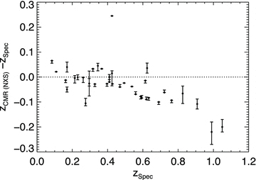
A comparison between photometric CMR redshifts obtained from NXS imaging (Section 2.2) and corresponding spectroscopic redshifts (Sections 2.3, 3.2 and 3.3). The comparison uses 39 clusters optically confirmed as gold or silver by ZooNXS (Section 4.1). Note that one of these 39 is not shown in the figure (XMMXCS J221559.6−173816.2), because it has an anomalously large redshift offset (see Table 6). The bars indicate the statistical 1σ limits on each CMR redshift (Section 2.2). Only those clusters with CMR redshifts obtained from photometrically calibrated data with a minimum of five galaxies and with statistical uncertainties of σz < 0.1 have been used in the comparison. The dotted line shows the one-to-one relation.
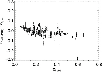
A comparison between photometric CMR redshifts obtained from SDSS DR7 imaging (Section 3.1) and corresponding spectroscopic redshifts (Sections 2.3, 3.2 and 3.3). The comparison uses 138 clusters optically confirmed as gold or silver by ZooDR7 (Section 4.1). The bars indicate the statistical 1σ limits on each CMR redshift (Section 2.2). Only those clusters with CMR redshifts obtained from a minimum of five galaxies and with statistical uncertainties of σz < 0.1 have been used in the comparison. The dotted line shows the one-to-one relation.
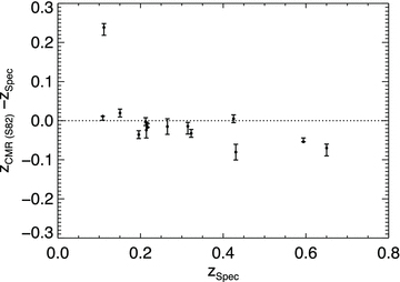
A comparison between photometric CMR redshifts obtained from the SDSS S82 (Section 3.1) and corresponding spectroscopic redshifts (Sections 2.3, 3.2 and 3.3). The comparison uses 14 clusters optically confirmed as gold or silver by ZooS82 (Section 4.1). The bars indicate the statistical 1σ limits on each CMR redshift (Section 2.2). Only those clusters with CMR redshifts obtained from a minimum of five galaxies and with statistical uncertainties of σz < 0.1 have been used in the comparison. The dotted line shows the one-to-one relation.
We note that a mean offset of Δz= 0.03, Δz= 0.01 and Δz= 0.02 was found for NXS, SDSS DR7 and S82, respectively, plus there is a trend to systematically underestimate CMR redshifts above zspec≃ 0.5 (Fig. 9). Given that the mean offsets are smaller than the statistical errors, and there are very few spectroscopic redshifts available beyond z≃ 0.5 with which to explore the redshift trend, we have not to adjust the CMR redshifts to compensate for them.
All of the 3σ redshift outliers are listed in Table 6. These outliers either represent catastrophic failures of the CMR technique or indicate incidences where the adopted spectroscopic redshift was wrong. In the following cases the CMR-redshift method has broken down: XMMXCS J133514.1+374905.8 and XMMXCS J221559.6−173816.2 (both clusters are at redshifts beyond the grasp of their respective imaging surveys). In the case of XMMXCS J163341.0+571420.1, the candidate lies right at the edge of the SDSS footprint, so that only a fraction of the extraction region contains catalogued SDSS galaxies; we will refine our CMR-redshift techniques to filter out such objects in future. In the remaining cases (XMMXCS J030644.2−000112.7, XMMXCS J033556.2+003214.7, XMMXCS J124100.8+325959.9 and XMMXCS J204134.7−350901.2), it is difficult to say if the fault lies with the CMR-redshift method or with the adopted spectroscopic redshift, as the zspec values are based on a single galaxy. More spectroscopy would be needed to confirm these redshifts, and hence improve our estimate of the CMR-redshift catastrophic failure rate. However, assuming all entries in Table 6 to be CMR failures, the failure rate is then ≃5, ≃3 and ≃7 per cent for NXS, SDSS DR7 and S82, respectively.
XCS clusters with CMR redshifts that were more than 3σ from their respective spectroscopic redshift. The XCS name is given in Column 1. The CMR redshift and the imaging survey from which it was derived are listed in Columns 2 and 3. The measured spectroscopic redshift and its source are given in Columns 4 and 5.
| XCS ID | zCMR value | Imaging survey | zspec | zspec source |
| (1) | (2) | (3) | (4) | (5) |
| XMMXCS J030644.2−000112.7 | 0.35 | S82 | 0.11 | LRG (Section 3.2) |
| XMMXCS J033556.2+003214.7 | 0.31 | DR7 | 0.43 | LRG (Section 3.2) |
| XMMXCS J124100.8+325959.9 | 0.15 | DR7 | 0.27 | LRG (Section 3.2) |
| XMMXCS J133514.1+374905.8 | 0.31 | DR7 | 0.60 | Literature (Section 3.3) |
| XMMXCS J163341.0+571420.1 | 0.54 | DR7 | 0.24 | Literature (Section 3.3) |
| XMMXCS J204134.7−350901.2 | 0.67 | NXS | 0.43 | XCS (Section 2.3) |
| XMMXCS J221559.6−173816.2 | 0.42 | NXS | 1.46 | XCS (Section 2.3) |
5.4 Selection of alternative names
Many of the XCS-DR1 clusters have been catalogued before by previous authors. In order to give due credit to this earlier work, we have matched XCS-DR1 clusters to catalogued clusters using an automated NED query. This query was run separately to that used to extract literature redshifts (Section 3.3) and involved a simple search for any NED object classified as a galaxy cluster within a fixed radius of the xapa-defined centroid. The radius used was the mean of the major and minor axes of the xapa defined source ellipse. In the event of several NED matches within this radius, the default top choice listed by NED (ordered by separation, on the date the query was made) was used. We concede that this approach is not ideal, in that it might not select the historical name of a cluster (e.g. one taken from the Abell catalogue, Abell 1958), if another catalogue (e.g. MaxBCG, Koester et al. 2007a) has an entry with an optical centroid closer to the xapa position. We also note that if the selected redshift (Section 5.2) of the XCS-DR1 cluster does not come from a literature source, then the redshift in XCS-DR1 might differ from the NED redshift for the previously catalogued cluster. In addition to the automated NED query, some alternative names have been added by hand from papers too recent to have been in NED at the time the search was carried out (see Section 3.3). In total, 247 of the XCS-DR1 clusters have been matched with alternative names.
6 SUMMARY AND DISCUSSION
In Fig. 1 we introduced the steps involved in the development of XCS-DR1. In this paper we have focused on the steps involving redshift follow-up, quality control and cluster catalogue compilation. In this section we summarize those aspects and highlight areas for future development.
6.1 Redshift follow-up (new observations)
In Section 2 we described new observations obtained to confirm XCS candidates as clusters and measure cluster redshifts. Section 2.1 focused on the methodology of the NXS (NOAO–XMM Cluster Survey) imaging programme and Section 2.2 presented the CMR-redshift method used to estimate redshifts from NXS galaxy catalogues. Over the course of 38 nights, a total of 415 candidates were targeted by NXS using the MOSAIC cameras at the KPNO and CTIO 4-m telescopes. Excluding unreliable fits, a total of 224 CMR-redshift measurements were made using NXS data, 73 of which appear in XCS-DR1. The accuracy and catastrophic failure rate of the NXS CMR redshifts were estimated to be σz= 0.08 and ≃5 per cent.
The original NXS goals were (i) to image, and derive CMR redshifts for, as many XCS candidates as possible, whilst (ii) also providing a useful data set for the X-ray community, i.e. deep imaging in two bands over a large number of XMM fields. With regard to our progress towards those goals, we are satisfied with the procedures used for NXS target selection, data reduction and photometric calibration. That said, it may be possible to improve the CMR-redshift accuracy, and reduce the catastrophic failure rate, by investigating different (to Bruzual & Charlot 2003) population synthesis models, to see if the redshift drift seen in Fig. 9 can be reduced. It might also be possible to improve the quality of the field galaxy sample used for the NXS CMR redshifts by using similarly sensitive archival data.
Looking ahead, we plan secure additional CCD imaging on 4-metre class telescopes. This will allow us to improve on, and extend, the current NXS results in three ways. First, we would like to calibrate the 30 NXS-fields that currently lack photometric calibration; this would allow additional CMR redshifts to be extracted from NXS. Secondly, there are hundreds of candidates that are yet to be included in an XCS-Zoo identification exercise to the depth of ZooNXS and ZooS82, including 467 candidates300 that have not been included in any XCS-Zoo, and a further 87 candidates300 that were classified as bronze in ZooDR7. As mentioned earlier (Section 4.1), we have already started the imaging follow-up of these objects. However we note that these new images will not be as useful to the X-ray community as those obtained during NXS, because they will not necessarily provide imaging across entire XMM field (for the new imaging campaigns, we are opting to target specific candidates). Thirdly, we could improve the accuracy of the existing CMR redshifts using additional observations through other filters. Other authors have shown that multi-colour photometric redshifts are more accurate than our single-colour ones. For example, Song et al. (2012) and High et al. (2010) achieve typical uncertainties of 2 per cent in Δz/(1 +z), to z < 0.5 and z < 1, respectively, using multi-colour data (both studies use the mean colour of the red-sequence as the cluster redshift estimator). Two other multi-colour cluster finders, MaxBCG and GMBCG (Koester et al. 2007a and Hao et al. 2010) achieve uncertainties of σz≃ 0.01 (z < 0.3) and σz= 0.015 (z < 0.55) respectively (both studies use the cluster red-sequence for cluster finding, but adopt the photometric redshift of the identified BCG as the cluster redshift). The addition of extra filters will mostly benefit the high-redshift end, but bluer filters would be of benefit at the low-redshift end also (i.e. allowing us to bridge the 4000 Å break at z < 0.3).
Section 2.3 presented the results to date (2011 June) from optical spectroscopy performed by XCS team members; 34 new (and one previously published) spectroscopic cluster redshifts (Table 2 and Table A1). We highlighted a new (to the literature) z > 1 cluster with multi-object spectroscopic confirmation (XMMXCS J091821.9+211446.0, z= 1.01, Fig. 3), and a new (to the literature) cluster, XMMXCS J015241.1−133855.9 at z= 0.83, that is most likely associated with the well-studied merger system XMMXCS J015242.2−135746.8 (or WARP J0152.7−1357). The new spectroscopic redshifts have been invaluable with regard to the calibration of the CMR redshifts and the derivation of X-ray temperatures. We intend to continue the spectroscopic follow-up of XCS candidates for several more years, with the emphasis on multi-object spectroscopy where possible.
6.2 Redshift follow-up (archive)
In Section 3, we described how we used data in public archives, and the literature, to collect more redshifts for our candidates (see Table 5 for a summary). In Section 3.1, we described how we applied the CMR-redshift technique designed for NXS to SDSS DR7 and S82 data. Excluding unreliable fits, a total of 574 and 51 CMR-redshift measurements were made using regular SDSS DR7 and S82 data, respectively, 80 and 19 of which appear in XCS-DR1. The accuracy (and catastrophic failure rates) of the SDSS CMR redshifts were estimated to be σz= 0.03 (≃3 per cent) and σz= 0.03 (≃7 per cent) for SDSS DR7 and S82, respectively. With regard to the future improvement of SDSS CMR redshifts, many of the statements made above, with regard to NXS, also apply here. However, in the case of SDSS, we already have the option of using more than one colour, so we are now investigating the use of multi-colour data to derive CMR redshifts from SDSS DR8. We also note that SDSS DR8 covers more area than DR7, so should yield additional (to XCS-DR1) redshifts.
In Section 3.2, we described how spectroscopic redshifts were extracted from the SDSS archive under the assumption that LRGs reside in the centres of X-ray clusters. A total of 265 spectroscopic redshifts were determined from SDSS LRGs, 111 of which appear in XCS-DR1. An additional three spectroscopic redshifts were adopted for XCS-DR1 clusters from the H12 XCS study. We look forward to the public release of additional SDSS spectroscopy from the SDSS-III Baryon Oscillation Spectroscopic Survey (BOSS) project,18 because this will allow us to extract more spectroscopic redshifts for XCS clusters.
In Section 3.3, we described how redshifts were extracted from the literature (mostly via automated queries to NED) and matched to XCS candidates. Whilst the use of zlits does cut down on the quantity of new optical follow-up required, it does have associated risks (i.e. that the selected redshift is not appropriate). Therefore, when assigning redshifts to clusters (if more than one redshift source was available), we tended not to use the NED-derived value. A total of 493 zlit values were collected from NED, of which 127 are presented in XCS-DR1. An additional 19 redshifts from literature sources are included in XCS-DR1, bringing the total to 142 (112 of these being spectroscopic in nature).
6.3 Quality control
In Section 4, we described the procedures used to confirm the identity of candidates as serendipitously detected clusters. In Section 4.1 we described an exercise, XCS-Zoo, that used the consensus opinion of at least five (of 23) volunteers to classify candidates. Those candidates classified as gold and silver were judged to have been ‘confirmed’ as clusters and appear in XCS-DR1. Those classified as bronze do not appear, unless additional information was available. In summary, 388 candidates were ‘confirmed’ as being clusters (i.e. were classified as gold or silver) using XCS-Zoo.
The remaining category, other, was used for candidates that did not fall into the gold, silver or bronze categories. Just over half of all candidates classified by XCS-Zoo were placed in this category. Subsequently to XCS-Zoo, we classified the other candidates300, finding that ≃25 per cent required more optical and/or X-ray follow-up before they could be identified (Section 4.1.1). The other ≃75 per cent could be removed from the candidate list without introducing incompleteness in the final XCS cluster sample. We described how we will be able to reduce, by a half, the number of contaminating objects entering candidate300 list in future (by improving the checks of reduced XMM images before xapa is run).
Overall, we feel that XCS-Zoo was a very worthwhile exercise. It has allowed us to efficiently identify several hundreds of X-ray clusters and has highlighted areas where the XCS candidate selection needs to be improved. We are planning to run XCS-Zoo again using additional (to NXS, S82 and DR7) data sets such as SDSS DR8, DSS, Canada–France–Hawaii Telescope Legacy Survey (CFHTLS) the Visible and Infrared Survey Telescope for Astronomy--Deep Extragalactic Observations Survey (VISTA-VIDEO) and the United Kingdom Infrared Telescope (UKIRT) Infrared Deep Sky Survey--Deep Extragalactic Survey (UKIDDS-DSS).19 For the next generation of XCS-Zoo we will include all candidates (i.e. not impose the >100 count threshold on ZooDR8, as it was in ZooDR7).
In Section 4.2 we described both how we interrogated the literature in order to confirm an additional 102 clusters and how we used our own spectroscopic follow-up to confirm 13 more. This process allowed us to confirm 18 bronze clusters from XCS-Zoo (Fig. 6), and several of those clusters have been included in the preliminary statistical subsample (Section 6.5.7). The remaining 97 clusters were not part of any XCS-Zoo and so they have a heterogeneous selection. These 97 have limited use with regard to statistical studies based on X-ray selection; however they still have value for other purposes, e.g. the study of individual interesting clusters (such as those at high redshift or under going mergers) or the interpretation of optically selected cluster catalogues. We note that of these 97 clusters, 87 have TX measurements in XCS-DR1 [whereas only 37 had a listed TX value in the X-Rays Clusters Database (BAX) at the time of writing].
In Section 4.3, we described checks that were made to ensure that ‘target’ clusters did not enter the XCS-DR1 sample; seven confirmed clusters were removed from XCS-DR1 as a result of these checks.
6.4 The cluster catalogue
In Section 5.1, we presented XCS-DR1 in the form of a table listing cluster attributes such as position, redshift, luminosity and X-ray temperature. In an associated webpage (http://www.xcs-home.org/datareleases), we also provide similar information together with optical and X-ray (colour-composite and grey-scale) images. In Section 5.2 we described the hierarchy used to select the best redshift for a cluster, if more than one estimate was available for it. In Section 5.3, we provided an estimate of the CMR-redshift errors and catastrophic failure rates. We found the errors to be similar to those obtained by other authors using similar, single-colour, techniques. As demonstrated in S09, errors and failure rates at the measured values should not significantly impact our ability to derive meaningful cosmological or evolutionary parameters.
We have found, using NED, that 247 (approximately half) of the XCS-DR1 clusters have been matched with previously catalogued clusters. This large fraction is a reflection of the fact that much of our redshift follow-up to date (2011 June) has come from the SDSS, and there are by now several optically selected cluster catalogues covering the SDSS footprint, e.g. MaxBCG (Koester et al. 2007a) and Cut-and-Enhance (Goto et al. 2002). As our optical follow-up continues, the percentage of previously reported clusters will fall, as evidenced by the fact that only 20 per cent (66 of 329) of the bronze objects from XCS-Zoo have matches to previously known clusters. Fig. 8 of S09 shows that XCS samples the cluster population well beyond the redshifts (z < 0.6) accessible to SDSS photometry, so the bronze category from ZooDR7 likely contains many of the distant clusters detected by XCS. It is noteworthy that few of the previously catalogued clusters in XCS-DR1 have been confirmed as X-ray clusters before. For example, we have compared XCS-DR1 to the BAX20 data base and found only 146 matches. Of these, only 55 (roughly a third) have previously published temperatures, i.e. XCS-DR1 presents TX values for 346 clusters for the first time. Indeed, there are only 394 clusters in BAX within the XCS-DR1 redshift (0.06 < z < 1.46) and temperature (0.4 < TX < 14.7 keV) ranges, compared to the 401 values released herein.
The XCS-DR1 cluster sample is distributed across the entire extra-Galactic sky and spans a wide range of redshift (Figs 12–15). In Figs 16, 17 and 18 we compare the XCS-DR1 redshifts and temperatures (values and errors) to previous data releases that have included X-ray cluster temperatures (Reiprich & Böhringer 2002; Pacaud et al. 2007; Maughan et al. 2008; Vikhlinin et al. 2009; Mantz et al. 2010). These show that XCS-DR1 not only contains many more cluster temperatures than previous work, but also probes higher redshifts and has a greater fraction of lower temperature systems.
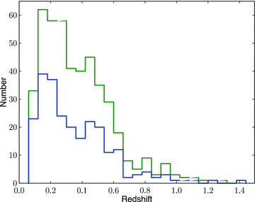
The redshift distribution for the 463 clusters with measured redshifts in XCS-DR1. The green line represents the total sample, while the blue line represents clusters300.
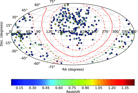
The distribution on the sky of the 463 clusters with measured redshifts in XCS-DR1. The green hashed lines represent the footprint of the DES. The colours of the dots represent the redshift of the cluster, as indicated.
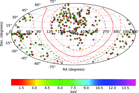
The distribution on the sky of the 401 clusters with measured X-ray temperatures in XCS-DR1. The green hashed lines represent the footprint of the DES. The colours of the dots represent the temperature of the cluster, as indicated.
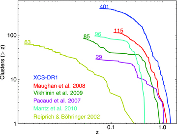
A comparison of the redshift distributions of XCS-DR1 clusters with previous data releases of X-ray cluster temperatures. The coloured numbers indicate the total number of clusters in the respective sample.
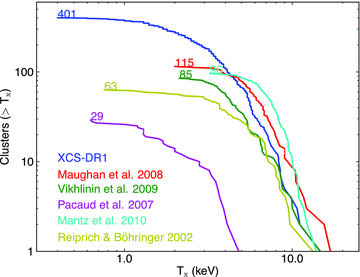
As for Fig. 16, but for the temperature distributions.
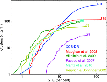
As for Fig. 16, but for the distribution of 1σ temperature errors.
Figs 19 and 20 show the distribution of X-ray temperature and luminosity (L500) with redshift for the XCS-DR1 sample. The XCS selection function is clearly evident in Fig. 20; the ability of xapa to detect low-luminosity clusters (particularly above the XCS minimum-count detection threshold) decreases with increasing redshift. This selection effect is less prominent with the Cluster300 sample.
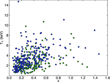
X-ray temperature plotted against redshift for the 401 clusters with measured temperatures in XCS-DR1. The green points represent the total sample, while the blue points represent clusters300.
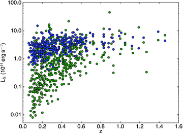
Bolometric (0.05–100 keV band) luminosity within a radius of R500 plotted against redshift for the 401 clusters with measured luminosities in XCS-DR1. The green points represent the total sample, while the blue points represent clusters300.
With the list of 503 confirmed clusters in place, we are continuing to improve the parameters we measure for each of them. For example, we are gathering additional spectroscopic data, and investigating the use of multi-colour CMR techniques, to improve the accuracy of the cluster redshifts. We also continue to monitor the literature to ensure we are using the best available published redshifts (rather than relying only on automated NED searches). Obtaining additional XMM observations of both those clusters300 with large (i.e. >20 per cent) TX errors, and those 15 clusters300 that failed the TX-pipeline entirely, will improve our X-ray temperature measurements. Follow-up of clusters that lie over CCD chip boundaries or on the edge of the field of view (see examples in Fig. 21) would allow us to improve luminosity measurements.
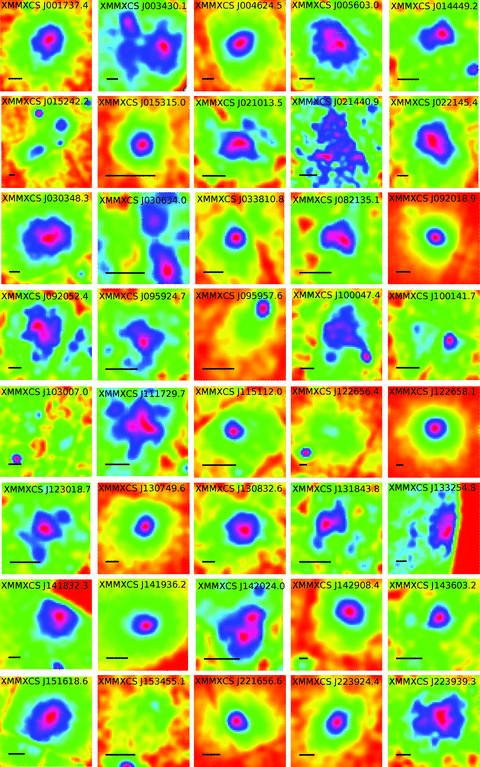
X-ray photon-count maps of 40 XCS-DR1 clusters detected with sufficient counts that it should be possible to measure X-ray temperature profiles. The names of the clusters are as indicated within the sub-panels. A scale of 100 kpc is indicated on each map by the horizontal black bar. Regions are coloured by the corresponding number of photon counts detected in XCS images based on a square-root scale (total source count values, and their coordinates, are provided in the electronic version of Table 3). Regions coloured in red (through to violet) correspond to regions detected with low (high) numbers of counts. Note that these are count, rather than count rate maps, i.e. they have not been corrected for variations in the exposure map. Several of the clusters lie over chip gaps, while others fall close to the edge of the field of view, hence some of the morphologies are artificially distorted. The ObsID images on the XCS-DR1 webpage provide a clearer impression of the exposure map variations.
We acknowledge that some XCS-DR1 clusters will suffer from contamination from line-of-sight, or embedded, point sources (including AGN and cool cores). In practice, contamination by high signal-to-noise ratio point sources is not a significant problem for XCS-DR1, because such sources are mostly distinguished by xapa from the cluster emission, e.g. in XMMXCS J011140.3−453908.0 and XMMXCS J022726.7−043209.1 (although, as the examples in Fig. 7 demonstrate, xapa does sometimes blend distinct XMM sources together). Rather, it is contamination by low signal-to-noise ratio point sources that concerns us; we have previously demonstrated (in Hilton et al. 2010, using Chandra follow-up) that the flux from XCS-DR1 cluster XMMXCS J221559.6−173816.2 (z= 1.46) was contaminated at the 15 per cent level by two point sources that had not been detected by xapa (although some issues pertaining to point-source detection are specific to xapa, Chandra is significantly more sensitive to point sources than XMM– although the reverse is true for extended emission – enabling these sources to be much more readily identified). Correcting for those point sources decreased the measured temperature by 2.4 keV (to  keV) and the luminosity by 33 per cent. To determine how common such low-level contamination might be (and the typical impact it has on derived parameters), we are undertaking an exercise that will make use of observations of XCS-DR1 clusters (and bronze candidates300) in the Chandra Data Archive.21 Using the Chandra Simple Image Access service, we have determined that 83 (23) of the XCS-DR1 clusters (bronze candidates300) are covered by Chandra observations (through to the end of 2009). These 83 XCS-DR1 clusters include 51 clusters300.
6.5 Selected subsamples of XCS-DR1 clusters
Finally, we describe seven subsamples of the XCS-DR1 clusters that have particular scientific applications. In each description we include methods that are being, or could be, used to improve and/or extend the respective subsample.
6.5.1 High-redshift XCS-DR1 Clusters
There are 10 clusters in Table 3 with z > 1.0. Of these clusters, all have been spectroscopically confirmed and are accompanied by TX measurements. By comparison, 16 (10 with TX measurements) z > 1.0 clusters were registered on the BAX data base at the time of writing (2011 June).
Although the BAX data base is not completely up to date, e.g. the z= 1.56 the XMM–Newton Distant Cluster Project (XDCP) cluster (XMMU J1007.4+1237; Fassbender et al. 2011) was not included at the time of writing, this comparison still demonstrates that the XCS-DR1 z > 1.0 cluster sample is the largest based on a single-selection technique (the 16 BAX clusters had been compiled from 11 different publications, with TX measurements from seven different publications). Most of the XCS-DR1 z > 1.0 clusters were previously known X-ray clusters, e.g. XMMXCS J223520.4−255742.1 at z= 1.39 (Mullis et al. 2005; Jee et al. 2009; Rosati et al. 2009). However, we highlight the two XCS discoveries: XMMXCS J221559.6−173816.2 (z= 1.46, previously published by us in Stanford et al. 2006) and XMMXCS J091821.9+211446.0 (z= 1.01, a spectroscopic redshift based on 16 galaxies; Fig. 3).
We plan to exploit the high-redshift XCS-DR1 clusters to extend our previous (Collins et al. 2009; Hilton et al. 2010; Stott et al. 2010) studies of galaxy, particularly BCG, evolution. Given the importance of high-z clusters to evolution studies, we will request additional X-ray follow-up (XMM and Chandra) of some of these clusters, in order to improve the signal-to-noise ratio and the spatial resolution. We are also working to extend the size of the XCS high-z sample. We are doing this in a number of ways, including: continuing the spectroscopic follow-up, using the Keck and Gemini telescopes, of promising high-z candidates that were highlighted during XCS-Zoo (regardless of the number of detected counts); using UKIDSS-DXS and VISTA-Video surveys to select additional high-z candidates; and exploiting redshifts measured by other teams, such as XDCP, for XMM clusters as they enter the literature.
6.5.2 High-temperature XCS-DR1 clusters
There are 66 clusters in XCS-DR1 with TX > 5 keV. This is a much smaller number than available on BAX (158 at the time of writing, 2011 June); however these clusters are still useful to the Sunyaev–Zeldovich community (SZ; Sunyaev & Zeldovich 1972) because typically it is only the TX > 5 keV clusters that can be detected via their SZ signal (using current instrumentation).
There are more TX > 5 keV clusters in BAX than in XCS-DR1 at all redshifts, but we note that at z > 0.5, the numbers are comparable: 30 clusters from XCS-DR1, compared to 39 in BAX. Of these, most (25) were not previously catalogued by BAX. Moreover, the 39 BAX clusters were drawn from a large number of different publications, whereas the XCS-DR1 sample is based on a single-selection technique and a single TX analysis method.
The XCS collaboration does not have direct access to SZ experiments, but targets have been supplied to the Atacama Pathfinder Experiment (APEX) and Arcminute Microkelvin Imager (AMI) teams (Zwart et al. 2008; Schwan et al. 2010), and several XCS-DR1 clusters have already been studied by the AMI SZ experiment (AMI Consortium: Shimwell et al., in preparation). In a separate publication (Viana et al. 2011) we present a subsample of XCS-DR1 clusters (including some at TX < 5 keV) that we predict will be detectable by the Planck SZ survey (Planck Collaboration et al. 2011).
Given the importance of high temperature clusters to SZ studies, and the fact that the accuracy of TX measurements drops with increasing temperature (see fig. 16 in LD11), it would be worthwhile to obtain additional X-ray observations of this sub-sample (regardless of the xapa count value), in order to increase the TX precision. Re-observing off-axis clusters at the XMM aim point, and/or with Chandra, will also increase the spatial resolution and allow us to correct for point source contamination (uncorrected AGN contamination will artificially raise the measured TX).
6.5.3 Low-temperature XCS-DR1 clusters
There are 130 clusters in XCS-DR1 with 0.4 < TX < 2 keV in the redshift range 0.06 < z < 1.46. This is dramatically more than in BAX (which lists only 27 such systems). We are already exploiting this unique data set to investigate AGN–intracluster medium (ICM) feedback mechanisms.
6.5.4 High signal-to-noise XCS-DR1 clusters
The XCS-DR1 TX values come primarily from the discovery data (the exception being those clusters that are both XMM targets and serendipitous detections; Section 4.3) and so the TX errors tend to be larger than the comparison samples, especially at the high-temperature/low-count end (Fig. 18). However, this is not always the case and, in particular, we note that there are 40 systems (Fig. 21) from which it should be possible to measure TX, to better than 15 per cent accuracy, in three or more radial bins (where these expectations are based on the results in LD11 concerning TX accuracy as a function of number of counts and TX). The 40 clusters featured in Fig. 21 comprise 23 clusters ranging in temperature from 2.6 < TX < 11.1 keV, and 17 groups ranging from 1.0 < TX < 1.8 keV.
The measurement of TX profiles will permit the measurement of cluster masses, under the assumption of hydrostatic equilibrium. This is important since mass calibration will be required before XCS-DR1 clusters can be used to constrain cosmological parameters (S09). We hope to increase the number of XCS-DR1 clusters with TX profiles by securing additional XMM observations. In particular, we wish to re-observe some systems that are representative of the LX–TX relation in the 1.8 < TX < 2.6 keV range (i.e. where there is a gap in the current high signal-to-noise ratio sample).
6.5.5 XCS-DR1 clusters in the Stripe 82 footprint
There are 35 clusters in XCS-DR1 that fall within the Stripe 82 (S82) co-add region of SDSS DR7. Of these, 27 have measured X-ray temperatures. The S82 region is of interest to many cluster scientists, primarily because it provides public high-quality imaging in several colours (≃2 mag deeper than regular SDSS) over a considerable area of sky. Optical cluster catalogues have been produced from S82 (e.g. Geach et al. 2011), but prior to XCS-DR1, there were only a handful of known X-ray clusters to use for S82 catalogue validation.
The Stripe 82 region will be re-observed by DES to similar depths and in the same bands. Therefore, the 27 XCS-DR1 clusters with TX measurements can be used immediately to investigate how DES-like cluster richnesses will correlate with the more reliable mass proxies.
6.5.6 XCS-DR1 clusters in the Dark Energy Survey footprint
In total, there are 100 XCS-DR1 clusters in the DES footprint (including the 35 in S82; Section 6.5.5). Of these, 77 have measured X-ray temperatures. All these clusters are worthy of further study (optical and X-ray) in order to support DES cluster science. The value of X-ray information about DES clusters has been demonstrated by Wu, Rozo & Wechsler (2010), who showed that with 200 follow-up observations, the dark energy figure of merit could be improved by 50 per cent. Although, with XCS-DR1, we have only been able to provide half that number, we note that there are several hundred more XCS cluster candidates in the DES footprint that are yet to be identified (as clusters or contaminants). Most of them have not been included in XCS-Zoo before, but their identification should be straightforward once DES photometry (which reaches a depth comparable to S82) is available. Given that DES photometry will cover several bands, it should be possible to measure accurate CMR redshifts for all DES-identified clusters.
We cannot at this stage predict how many of the DES-identified clusters will yield TX values, but we note that the number of unidentified candidates300 in the DES footprint is 156. In addition, we are applying the XCS X-ray analysis pipelines to an additional ≃40 clusters with XMM detections. These additional clusters are not in our candidate list, because they were the targets of their respective ObsID; however, they are still very useful to DES because they will help us reach the Wu et al. (2010) target of 200. These 40 are likely to be particularly useful to DES since many will have been detected with sufficient signal-to-noise ratio to yield mass estimates via the hydrostatic equilibrium method.
6.5.7 XCS-DR1 clusters for statistical studies
Although the optical follow-up of XCS300 is still ongoing, we have nevertheless been able to define a subsample of XCS-DR1 clusters that should be sufficiently complete to be suitable for preliminary statistical studies. For this we have only used clusters300 that were classified by XCS-Zoo and optically confirmed. We confined the sample to the redshift range that should yield CMR redshifts from the respective imaging (i.e. z < 0.3 for ZooDR7 and z < 0.6 for ZooNXS and ZooS82– refer to Figs 2, 8 and 22 to see how the galaxy density changes with cluster redshift and survey depth). We also impose a lower redshift cut of z > 0.1, because this is the minimum allowed by the CMR algorithm.
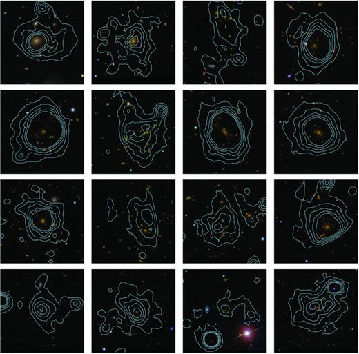
A selection of optically confirmed XCS clusters as imaged by SDSS DR7 and classified as gold in ZooDR7 (Section 4.1). False colour-composite images are 3 × 3 arcmin with X-ray contours overlaid in blue. From left to right and top to bottom, the compilation displays the clusters: XMMXCS J115112.0+550655.5 at z= 0.08; XMMXCS J010858.7+132557.7 at z= 0.15; XMMXCS J123019.6+161634.1 at z= 0.20; XMMXCS J001737.4−005235.4 at z= 0.21; XMMXCS J092018.9+370617.7 at z= 0.21; XMMXCS J100047.4+013926.9 at z= 0.22; XMMXCS J083454.8+553420.9 at z= 0.24; XMMXCS J130749.6+292549.2 at z= 0.24; XMMXCS J170041.9+641257.9 at z= 0.24; XMMXCS J133254.8+503153.1 at z= 0.28; XMMXCS J092052.4+302804.8 at z= 0.29; XMMXCS J141832.3+251104.9 at z= 0.29; XMMXCS J105318.5+572043.7 at z= 0.34; XMMXCS J115824.6+440533.9 at z= 0.41; XMMXCS J153629.7+543920.8 at z= 0.41 and XMMXCS J111515.6+531949.5 at z= 0.47.
Setting these limits, we have selected a total of 104 clusters300, of which 69 come from ZooDR7 and an additional 35 come from ZooNXS or ZooS82. To put this sample into context, we can compare it to the influential study by Vikhlinin et al. (2009) that used 88 clusters (49 in the range 0.025 < z < 0.2 and 39 in the range 0.35 < z) to derive constraints on dark energy parameters.
We hope the sample will be widely used by the community, and have indicated the 104 members in Table 3. However, we stress that it is not applicable for all types of statistical studies, because it is not complete: some clusters in the selected redshift range will not have been ‘confirmed’ yet and so do not appear in XCS-DR1. We do not know how many such clusters are there, but we estimate the number to be ≃50; there are 40 bronze clusters300 and nine other candidates300 with CMR redshifts in the respective ranges (where the other candidates300 are in the sub-categories that ‘require additional follow-up’; Section 4.1.1). Assuming all 49 are clusters, then the current sample of 104 is only 69 per cent complete. Moreover, this sample cannot be used without reference to the XCS survey selection function (LD11) for science applications that require the volume density to be known. In future publications, we will apply this sample to a variety of investigations, e.g. the derivation of cosmological parameters and the measurement of cluster scaling relations. The scaling relations we plan to examine are those between: X-ray luminosity and TX; optical richness and TX; and halo occupation number and TX.
We look forward to increasing the size, and completeness level, of future ‘statistical’ sub-samples of XCS clusters using the DES. The combination of DES and XCS will yield a homogeneously selected set of confirmed X-ray clusters that is at least twice the size of the current statistical sub-sample. It is important to note, in this context, that the fraction of bronze and other systems in the similarly (to DES) deep S82 region is significantly lower than that in the DR7 region. Extrapolating from the ZooS82 results, we expect completeness levels of XCS cluster samples in the DES region to be at least 80 per cent. If the Pan-Starrs422 project is successful, then even larger samples could be gathered because that optical survey will cover the whole sky north of −30°, to similar depths to DES.
7 CONCLUSIONS
We have presented the first data release from the XCS (XCS-DR1). This consists of 503 optically confirmed X-ray clusters serendipitously detected in XMM archival imaging. Optical confirmation was established in one or more of three ways: through multi-object spectroscopy; by matching XCS candidates to clusters in the literature or by visual inspection of optical CCD images via an exercise referred to as XCS-Zoo. Redshifts for the clusters were derived from a variety of spectroscopic and photometric sources, namely public archives, the literature and our own follow-up campaigns. X-ray temperatures and luminosities were measured for those clusters detected with sufficient signal-to-noise ratio using an automated pipeline. We have established whether the clusters (and/or their X-ray temperature measurements) are new to the literature using comparisons with NED and BAX. Compared to previous data releases of cluster samples with TX information, XCS-DR1 contains more clusters (especially at low temperature) and probes to higher redshifts. The XCS-DR1 catalogue, together with optical (colour-composite and grey-scale) and X-ray imaging for each of the XCS-DR1 clusters, is publicly available from http://www.xcs-home.org/datareleases.
Some key statistics for the XCS-DR1 catalogue of 503 clusters are as follows.
Redshifts: 463 clusters are accompanied by redshift information (0.06 < z < 1.46). Of these, 261 are spectroscopic, with most of the remainder coming from the photometric CMR-redshift technique (applied to single-colour optical imaging). 10 of the redshifts exceed z= 1.0 (these include a new spectroscopically confirmed cluster at z= 1.01). The CMR-redshift accuracy (and catastrophic failure rates) were found to be σz= 0.08 (≃5 per cent), σz= 0.03 (≃3 per cent) and σz= 0.03 (≃7 per cent) from NXS, SDSS DR7 and Stripe 82 data, respectively.
Temperatures: 401 clusters are accompanied with X-ray temperature information (0.4 < TX < 14.7 keV). Of these, 66 clusters have temperatures above TX= 5 keV (these systems will be particularly useful for SZ studies), and 130 clusters have temperatures below TX= 2 keV (these systems can be applied to studies of cluster physics and BCG evolution). A small subset, of 40 clusters, were detected with sufficient signal-to-noise ratio that mass measurements can be made using temperature profiles (these will be important to cosmology studies, as they will aid the mass calibration of XCS). Those clusters presented with TX values are also presented with LX measurements.
New discoveries/measurements: 256 clusters were not previously catalogued in the literature, and 357 of the X-ray temperature measurements were not previously catalogued in BAX.
Preliminary statistical subsample: of the 503 XCS-DR1 clusters, 104 can be used, in conjunction with the XCS selection function, for statistical applications such as the derivation of cosmological parameters and the measurement of cluster scaling relations (including those between X-ray luminosity and TX, and optical richness and TX).
We thank an anonymous referee for their careful reading of the manuscript and for their insightful comments and suggestions. We also thank Ben Maughan for advice regarding X-ray temperature profiles and a Wide Angle ROSAT Pointed Survey (WARPS) cluster redshift, and Monique Arnaud for advice regarding her investigations of XCS-DR1 clusters in PXCC. NM thanks Chris Wegg for useful discussions on the CMR-redshift method.
We are most grateful to the support staff who operate the following observatories and to the organizations that fund them: the ESA XMM–Newton mission. The NOAO consists of KPNO near Tucson, Arizona, CTIO near La Serena, Chile, and the NOAO Gemini Science Center. NOAO is operated by the Association of Universities for Research in Astronomy (AURA) under a cooperative agreement with the National Science Foundation. The Gemini Observatory, which is operated by the Association of Universities for Research in Astronomy, Inc., under a cooperative agreement with the National Science Foundation (NSF) on behalf of the Gemini partnership: the National Science Foundation (United States), the Science and Technology Facilities Council (United Kingdom), the National Research Council (Canada), CONICYT (Chile), the Australian Research Council (Australia), Ministrio da Cincia e Tecnologia (Brazil) and Ministerio de Ciencia, Tecnologa e Innovacin Productiva (Argentina). The Keck Observatory. The analysis pipeline used to reduce the DEIMOS data was developed at UC Berkeley with support from NSF grant AST-0071048. The authors wish to recognize and acknowledge the very significant cultural role and reverence that the summit of Mauna Kea has always had within the indigenous Hawaiian community; we are fortunate to have the opportunity to conduct observations from this mountain. The W. M. Keck Observatory is a scientific partnership between the University of California and the California Institute of Technology, made possible by a generous gift of the W. M. Keck Foundation. The NTT ESO Telescope at the La Silla Observatory under programmes 077.A-0437, 078.A-0325, 080.A-0024, 081.A-843. The William Herschel Telescope which is operated on the island of La Palma by the Isaac Newton Group in the Spanish Observatorio del Roque de los Muchachos of the Instituto de Astrofísica de Canarias.
We also acknowledge the following public archives, surveys and analysis tools: the SDSS. Funding for the SDSS and SDSS-II has been provided by the Alfred P. Sloan Foundation, and a wide variety of the Participating Institutions (see http://www.sdss.org for details). The DSS produced at the Space Telescope Science Institute under U.S. Government grant NAG W-2166. The NED which is operated by the Jet Propulsion Laboratory, California Institute of Technology, under contract with the National Aeronautics and Space Administration. The Chandra Data Archive (cxc.harvard.edu/cda). The iraf reduction pipeline distributed by the National Optical Astronomy Observatories, which are operated by the Association of Universities for Research in Astronomy, Inc., under cooperative agreement with the National Science Foundation. The X-Ray Clusters Database (BAX) which is operated by the Laboratoire d’Astrophysique de Tarbes-Toulouse (LATT), under contract with the Centre National d’Etudes Spatiales (CNES). Montage, funded by the National Aeronautics and Space Administration’s Earth Science Technology Office, Computation Technologies Project, under Cooperative Agreement Number NCC5-626 between NASA and the California Institute of Technology. Montage is maintained by the NASA/IPAC Infrared Science Archive. GAIA is a derivative of the Skycat catalogue and image display tool, developed as part of the VLT project at ESO. Skycat and gaia are free software under the terms of the GNU copyright.
Financial support for this project includes: The Science and Technology Facilities Council (STFC) through grants ST/F002858/1 and/or ST/I000976/1 (for EL-D, AKR, NM, MHo, ARL and MS), ST/H002391/1 and PP/E001149/1 (for CAC and JPS), ST/G002592/1 (for STK) and through studentships (for NM, HCC), ST/H002774/1 and ST/I001204/1 (for EME) The University of KwaZulu-Natal (for MHi). The Leverhulme Trust (for MHi). The University of Sussex (MHo, HCC, PD). FP7-PEOPLE- 2007-4Ð3-IRG n 20218 (for BH). Fundação para a Ciência e a Tecnologia through the project PTDC/CTE-AST/64711/2006 (for PTPV). The South East Physics Network (for RCN, END, WAW). The Swedish Research Council (VR) through the Oskar Klein Centre for Cosmoparticle Physics (for MS). The RAS Hosie Bequest and the University of Edinburgh (for MD). The U.S. Department of Energy, National Nuclear Security Administration by the University of California, Lawrence Livermore National Laboratory under contract No. W-7405-Eng-48 (for SAS). The Greek State Scholarship Foundation, trustee of the Nik. D. Chrysovergis legacy (for LC). Parts of the manuscript were written during a visit by AKR to the Aspen Physics Center.
Footnotes
xmm.esac.esa.int
Information and a Data Handbook which describes how to access NOAO archival data and use the NOAO Portal is available at: http://www.noao.edu/sdm/help.php
The pipeline implements a Master sky-flat generated from every science frame taken at the CTIO 4-m telescope and produces pre-stacked, sky-flattened, World Coordinate System (WCS) corrected images.
Satellite trails were masked using the script sat-b-gon.pl written by Matthew Hunt, available from http://www.ifa.hawaii.edu.
star-http://www.dur.ac.uk/pdraper/gaia/gaia.html
During the preparation of this manuscript, the SDSS Eighth Data Release was made public (DR8; Aihara et al. 2011). Importantly, this covers more area than SDSS DR7, so we will be exploiting SDSS DR8 for XCS follow-up in future publications.
In principle, as was the case for the LRG redshifts (Section 3.2), we would have been prepared to assign zlit < 0.08 values to clusters if the measured CMR redshift pegged at the algorithm’s minimum value (z= 0.1). However, in practice there were no such candidates.
In principle, useful information related to candidate identification could be derived from a wide range of observations, including radio and infrared, but to date (2011 June) we have only used optical data.
All XCS candidates are extended in a statistical sense, but only the high signal-to-noise ratio sources stand out to the human eye as being unambiguously extended and without blend contamination.
The slight decrease compared to the numbers mentioned in the paragraph above is a result of the removal of some clusters that were either ObsID targets or associated with ObsID targets (Section 4.3).
Images of this object are not available from http://www.xcs-home.org/datareleases because it is not part of XCS-DR1. Please contact the authors for more information.
Jupiter did originally appear in our list of other candidates and, because it does not have a fixed location on the sky, did not have an SDSS counterpart. Even so, it was still identifiable, as not being a cluster, on the basis of its peculiar X-ray profile.
REFERENCES
Appendix
APPENDIX A: INDIVIDUAL GALAXY SPECTROSCOPIC REDSHIFTS
Spectroscopic redshifts of individual cluster galaxies acquired by XCS team members (see Table 2). The respective XCS-DR1 cluster name is listed under ‘XCS ID’. Note that redshifts obtained during Gemini GMOS campaigns are not included, but will be presented in Hilton et al. (in preparation).
| XCS ID | RA (○) | Dec. (○) | z |
| XMMXCS J011140.3−453908.0 | 17.88713 | −45.64071 | 0.368 |
| XMMXCS J011140.3−453908.0 | 17.90525 | −45.64579 | 0.369 |
| XMMXCS J011140.3−453908.0 | 17.90689 | −45.64270 | 0.369 |
| XMMXCS J011140.3−453908.0 | 17.91184 | −45.66472 | 0.367 |
| XMMXCS J011140.3−453908.0 | 17.91186 | −45.66474 | 0.367 |
| XMMXCS J011140.3−453908.0 | 17.91604 | −45.65496 | 0.365 |
| XMMXCS J011140.3−453908.0 | 17.92272 | −45.65455 | 0.369 |
| XMMXCS J011140.3−453908.0 | 17.93787 | −45.64076 | 0.366 |
| XMMXCS J011140.3−453908.0 | 17.94503 | −45.69240 | 0.367 |
| XMMXCS J011140.3−453908.0 | 17.94613 | −45.66257 | 0.369 |
| XMMXCS J011140.3−453908.0 | 17.95873 | −45.68057 | 0.363 |
| XMMXCS J012400.0+035110.8 | 21.00450 | +3.85052 | 0.8851 |
| XMMXCS J012400.0+035110.8 | 21.00081 | +3.86062 | 0.8815 |
| XMMXCS J012400.0+035110.8 | 20.99229 | +3.86113 | 0.8807 |
| XMMXCS J012400.0+035110.8 | 21.01021 | +3.85791 | 0.8845 |
| XMMXCS J012400.0+035110.8 | 21.01319 | +3.84871 | 0.8848 |
| XMMXCS J012400.0+035110.8 | 20.99180 | +3.84015 | 0.8840 |
| XMMXCS J012400.0+035110.8 | 21.03991 | +3.77769 | 0.8802 |
| XMMXCS J015241.1−133855.9 | 28.18386 | −13.56996 | 0.8140 |
| XMMXCS J015241.1−133855.9 | 28.18410 | −13.58052 | 0.8209 |
| XMMXCS J015241.1−133855.9 | 28.16310 | −13.67646 | 0.8213 |
| XMMXCS J015241.1−133855.9 | 28.16573 | −13.64554 | 0.8222 |
| XMMXCS J015241.1−133855.9 | 28.16405 | −13.64879 | 0.8232 |
| XMMXCS J015241.1−133855.9 | 28.17766 | −13.64977 | 0.8259 |
| XMMXCS J015241.1−133855.9 | 28.18081 | −13.64001 | 0.8348 |
| XMMXCS J015241.1−133855.9 | 28.17865 | −13.64028 | 0.830 |
| XMMXCS J015241.1−133855.9 | 28.16838 | −13.63908 | 0.8297 |
| XMMXCS J015241.1−133855.9 | 28.16465 | −13.66412 | 0.8211 |
| XMMXCS J015241.1−133855.9 | 28.17508 | −13.64465 | 0.83 |
| XMMXCS J023346.0−085048.5 | 38.44672 | −8.84924 | 0.25 |
| XMMXCS J030317.4+001238.4 | 45.82094 | +0.20800 | 0.594 |
| XMMXCS J032553.3−061719.9 | 51.47002 | −6.28611 | 0.3212 |
| XMMXCS J032553.3−061719.9 | 51.47681 | −6.28504 | 0.3242 |
| XMMXCS J035417.0−001006.6 | 58.57171 | −0.16705 | 0.2140 |
| XMMXCS J035417.0−001006.6 | 58.57550 | −0.16409 | 0.2148 |
| XMMXCS J041944.6+143904.5 | 64.93533 | +14.65633 | 0.19310 |
| XMMXCS J041944.6+143904.5 | 64.93400 | +14.65807 | 0.19292 |
| XMMXCS J045506.3−532343.8 | 73.77404 | −53.39641 | 0.410 |
| XMMXCS J051610.0+010954.0 | 79.04254 | +1.16779 | 0.3184 |
| XMMXCS J051610.0+010954.0 | 79.04033 | +1.16780 | 0.3182 |
| XMMXCS J080612.6+152309.0 | 121.55758 | +15.38483 | 0.41 |
| XMMXCS J095105.7+391742.9 | 147.78329 | +39.29456 | 0.47 |
| XMMXCS J102136.9+125643.2 | 155.40917 | +12.95153 | 0.325 |
| XMMXCS J130601.4+180145.9 | 196.49959 | +18.02754 | 0.9259 |
| XMMXCS J130601.4+180145.9 | 196.51167 | +18.03038 | 0.9214 |
| XMMXCS J130601.4+180145.9 | 196.52493 | +18.01557 | 0.9348 |
| XMMXCS J150652.9+014424.8 | 226.72214 | +1.7423 | 0.652 |
| XMMXCS J150652.9+014424.8 | 226.72562 | +1.7418 | 0.65369 |
| XMMXCS J153643.9−141024.2 | 234.17675 | −14.17587 | 0.407 |
| XMMXCS J153643.9−141024.2 | 234.18551 | −14.17263 | 0.397 |
| XMMXCS J200703.1−443757.6 | 301.76587 | −44.63324 | 0.202 |
| XMMXCS J204134.7−350901.2 | 310.37374 | −35.14911 | 0.42508 |
| XMMXCS J212807.6−445417.3 | 322.02520 | −44.90470 | 0.544 |
| XMMXCS J212807.6−445417.3 | 322.04503 | −44.90863 | 0.535 |
| XMMXCS J212807.6−445417.3 | 322.07628 | −44.88251 | 0.536 |
| XMMXCS J212807.6−445417.3 | 322.12141 | −44.87643 | 0.538 |
| XMMXCS J231852.3−423147.6 | 349.71571 | −41.47931 | 0.114 |
| XMMXCS J235708.6−241449.2 | 359.26616 | −24.25600 | 0.588 |
| XMMXCS J235708.6−241449.2 | 359.26643 | −24.25617 | 0.586 |
| XMMXCS J235708.6−241449.2 | 359.27353 | −24.24871 | 0.588 |
| XMMXCS J235708.6−241449.2 | 359.27690 | −24.25285 | 0.588 |
| XMMXCS J235708.6−241449.2 | 359.27986 | −24.25803 | 0.587 |
| XMMXCS J235708.6−241449.2 | 359.28441 | −24.22818 | 0.587 |
| XMMXCS J235708.6−241449.2 | 359.29057 | −24.27279 | 0.5903 |
| XMMXCS J235708.6−241449.2 | 359.29073 | −24.24162 | 0.58657 |
| XMMXCS J235708.6−241449.2 | 359.29206 | −24.24552 | 0.588 |
| XMMXCS J235708.6−241449.2 | 359.31111 | −24.17266 | 0.592 |
SUPPORTING INFORMATION
Additional Supporting Information may be found in the on-line version of this article:
Table 1. Summary of NXS observations.
Tables 3 and 4. The XCS-DR1 Cluster Catalogue: Part II, X-ray luminosities.
Please note: Wiley-Blackwell are not responsible for the content or functionality of any supporting materials supplied by the authors. Any queries (other than missing material) should be directed to the corresponding author for the article.
