Building up the spectrum of cosmic rays in star-forming regions

Abstract

1 INTRODUCTION

From radio to TeV gamma-rays, starbursts shine in the sky. Their large star formation rates power high-injection rates of cosmic rays (CRs) in the interstellar media of these galaxies, which emit non-thermal radiation. The large CR energy contents in starbursts are of interest for CR feedback (Socrates, Davis & Ramirez-Ruiz 2008), ionization (Papadopoulos 2010), the gamma-ray background (e.g. Thompson, Quataert & Waxman 2007; Makiya, Totani & Kobayashi 2011) and for determining whether they are neutrino sources (e.g. Loeb & Waxman 2006). Indeed, the large cosmic content has been supported by the recent detections of M82 and NGC 253 by GeV and TeV telescopes (Acciari et al. 2009; Acero et al. 2009; Abdo et al. 2010). In anticipation and as spin-off of these detections, there has recently been a spate of modelling of the CR spectrum in starburst galaxies.

In considering the CR spectrum in star-forming regions, models generally start by writing the diffusion-loss equation (see e.g. Ginzburg & Syearovatskii 1964)

1

where N(E) is the distribution of particles with energies in the range E and E+ d E per unit volume, and b(E) =−(dE/dt) is the rate of loss of energy. In this equation, D is the scalar diffusion coefficient, Q(E) represents the source term appropriate to the production of particles with energy E and τ(E) is the residence time (beyond which particles are removed from the phase space). It is usually assumed that the starburst is in a steady state, and, under the assumption of a homogeneous distribution of sources, that the spatial dependence can be ignored, so that D∇²N(E) = 0. These assumptions were adopted by essentially all detailed models of starburst regions published in the literature so far (e.g. see Paglione et al. 1996; Blom, Paglione & Carramiana 1999; Torres 2004; Domingo-Santamaría & Torres 2005; de Cea del Pozo, Torres & Rodriguez-Marrero 2009; Lacki, Thompson & Quataert 2010, and references therein). Persic, Rephaeli & Arieli (2008) and Rephaeli, Arieli & Persic (2010) solve the diffusion–convection equation in 3D, but do not discuss the detailed spatial distribution of CRs, just the average spectrum over the starburst and the surrounding disc. This was also the case for some of the formerly quoted papers. On the other hand, the galprop models (see Strong & Moskalenko 1998) for the propagation of CRs in our Galaxy do not consider the formation of the CR spectrum from the individual contributors, in a time-dependent manner.

In the previously mentioned models, and in regard to equation (1), the proton injection is assumed to be a power law with index p, for instance,

2

where K is a normalization constant and units are such that [Q] = GeV⁻¹ cm⁻³ s⁻¹. The proton injection is assumed to be uniform across the starburst. The power-law spectrum follows from the results of Fermi first-order acceleration assumed for individual accelerators (e.g. Bell 1978; see also Ellison, Decourchelle & Ballet 2004). The normalization is obtained from the total power transferred by supernovae into the CR kinetic energy within a given volume,

3

where, for simplicity, p≠ 2 was assumed, and we used the fact that E_{p, kin, min}≪E_{p, kin, max} in the second equality. The last part of equation (3) is simply the total power using (⁠⁠) as the rate of supernova (SN) explosions in the star-forming region of volume V that releases a fraction η_i of its power into relativistic CRs. We note that non-linear theories of CR acceleration predict deviations from the power-law injection spectrum, especially at low energies and near the high-energy cutoff (e.g. Berezhko & Ellison 1999; Ellison, Berezhko & Baring 2000). In addition, Ptuskin & Zirakashvili (2005) argue that at any given time, only particles near an evolving cut-off energy actually escape the SN remnant, and only the time-averaged injection spectrum is a power law (see also Fujita et al. 2009; Fujita, Ohira & Takahara 2010). Thus, the spectrum and time evolution of CR accelerators may be more complicated than we consider here.

The injection spectrum of the primary particles [Q(E), from which one derives the distribution N(E) and then e.g. the gamma-ray emission] is assumed to be directly normalized by the total SN explosions in the galaxy, and to have a power-law form with fixed index, irrespective of position within the starburst. The common approach is then equivalent to assuming that at any point of the starburst region, there is a single accelerator inputting CRs at a reduced rate, one that is compatible with the overall volume average given by the total number of accelerators. How realistic are all these assumptions?

There are direct observational hints that the luminosity in gamma-rays is correlated with the star formation rate (from now on, SFR) or SN frequency. The correlation may be slightly non-linear, following a power law with a hard index, L_γ∼ SFR^b, with b∼ 1–1.4 (Abdo et al. 2010). Due to the current scarcity of starbursts measured in gamma-rays, this is, however, not yet proven. Strictly speaking, this relation is in fact impossible to predict in the models presented in the literature so far, since the SFR goes into the normalization of the primary CR spectrum, which is assumed. Then, it is natural to expect that to first order, the same correlation is maintained in the hadronic gamma-ray luminosity generated by the former population. Plots such as L_γ versus SFR (or similarly, enhancement of CRs versus SFR) have not been derived (to our knowledge) from first principles yet.

We also note that the problem of calorimetric (essentially, full conversion of the proton kinetic energy into secondary particles like gamma-rays) or non-calorimetric behaviour also depends on the validity of the assumption of the primary spectrum, emphasizing that an understanding of how it is built up from individual contributors could be useful.

The aim of this work is then to assess some of the formerly commented common assumptions made in the description of the injected CR spectrum of starburst regions, by accounting for the individual contributions of accelerators residing in the starburst volume over the starburst age.

2 NUMERICAL APPROACH AND RESULTS

As stated, instead of considering a total, volume-averaged, CR injection, we shall obtain the individual contribution of each accelerator to the CR intensity at a given time. The CR intensity contribution of each of the accelerators will thus be given by

4

where f(E, r, t) is the distribution function of protons at time t and distance r from the source which satisfies the radial–temporal–energy-dependent diffusion equation

5

(we choose spherical coordinates, with r being the radial distance from a given accelerator and P representing the energy losses). We should note the differences between the simplified equation (1), for the whole starburst, and equation (5). The latter is written for a single accelerator, and thus, Q is the injection of CRs of that accelerator only and is obviously more constrained. Note also that equation (5) refers to an E-, r- and t-dependent problem, whereas after the simplifications of equation (1) that we mentioned above, it is homogeneous and in a steady state, and thus only E dependent. But we note a caveat too: in order to work with analytically tractable solutions of equation (5), see below, we ignored the advective escape term [i.e. N(E)/τ(E)]; thus, we do not consider here outflows that may remove CRs from the starburst regions. CRs are transported here by diffusion, which is appropriate in the calorimetric limit only (see, e.g., Loeb & Waxman 2006; Thompson et al. 2007).

We assume that the proton energy loss is due to nuclear interactions. The nuclear loss rate is ⁠, where is the time-scale for the corresponding nuclear loss, κ∼ 0.45 is the inelasticity of the interaction and mb is the cross-section (e.g. Stecker 1971; Gaisser 1990); is essentially constant for the energies of interest above GeV. Thus, following e.g. Aharonian & Atoyan (1996), yr. The solution to the diffusion equation for an arbitrary energy loss term, diffusion coefficient and impulsive injection spectrum f_inj(E), such that ⁠, for the particular case in which D(E) ∝E^δ and f_inj∝E^−α, is (see Aharonian & Atoyan 1996, and references therein)

6

where

7

stands for the radius of the sphere up to which the particles of energy E have time to propagate after their injection. In the case of continuous injection of accelerated particles, given by ⁠, the previous solution needs to be convolved with the function in the time interval 0 ≤t′≤t. If the source is described by a Heaviside function, the solution is (Atoyan, Aharonian & Völk 1995)

8

All previous equations in this section are thus valid for a single accelerator, e.g., a single SN remnant or pulsar wind nebula, injecting either impulsively or continuously CRs into the starburst. We now consider that a starburst is a collection of such accelerators, which are assumed to appear in the starburst volume at a given rate, e.g., equal to the SN rate (which is in turn related to the SFR), and which could be constant (as is usually assumed) or not (e.g., the starburst phenomenon could have ended, or it could be a short burst of star formation rather than a continuous one). Thus, one can consider the evolution in time of the injection spectrum of the whole starburst by computing each accelerator’s contribution using the solution to equation (5), and solving it as many times as there are injectors in the volume.

This concept is depicted in Fig. 1. Each plane represents a given past time in the evolution of the starburst (the current time is t₃ in that figure). Each test region of the starburst today receives the CR contribution of each of the accelerators injecting CRs in its past, for which we individually consider the propagation from the time of its injection up to the test region. Summing up all contributions, we build up the spectrum at that point. Comparing different test points we can check for homogeneity, and study, for instance, how many and which are the accelerators contributing mostly to the total spectrum. One consequence of such an approach to compute the total spectrum is a direct relation between the accelerator appearance rate and the CR intensity in a given position. By slicing in time and space bins from that test position, the number of accelerators in each bin will, under a homogeneous and isotropic distribution, be directly proportional to the accelerator appearance rate. (Each of the panels in Fig. 1 will have as many accelerators as determined by the appearance rate assumed.) Such proportionality would be apparent in the CR intensity, since, for sufficiently small time and space bins, the differences among the contributions of accelerators that were born in that bin will be negligible; this would lead to a linear relationship between CR intensity and accelerators’ appearance rate. We have checked that this is indeed the case in our numerical simulations.

Figure 1

Concept for the computation of individual contributions of the CR density in star-forming regions.

Open in new tabDownload slide

2.1 Cosmic ray injection from a single accelerator

As an example of the results, we consider first the injection of a single accelerator. We show in Fig. 2 the CR intensity contribution for an injection that occurred at different times in the starburst history and at different distances from the test point. We consider here (as we do below) that the diffusion coefficient at 10 GeV is 10²⁶ cm² s⁻¹ and δ= 0.5 in a medium of density n= 35 cm⁻³; we have also explored other parameter values. A low value of diffusion coefficient (slow diffusion) is expected in dense molecular regions, such as a starburst [see e.g. the cases of dense molecular clouds in our Galaxy in the works by Ormes, Ozel & Morris (1988); Gabici (2010); Torres, Rodriguez-Marrero & de Cea del Pozo (2010), and other references therein]. With the selected value of interstellar particle density, the total molecular mass in a typical starburst sphere of 300 pc is ∼10⁸ M_⊙. Times considered are 10⁴, 10⁵ and 5 × 10⁵ yr and distances considered are 10, 50 and 100 pc from the test point.

Figure 2

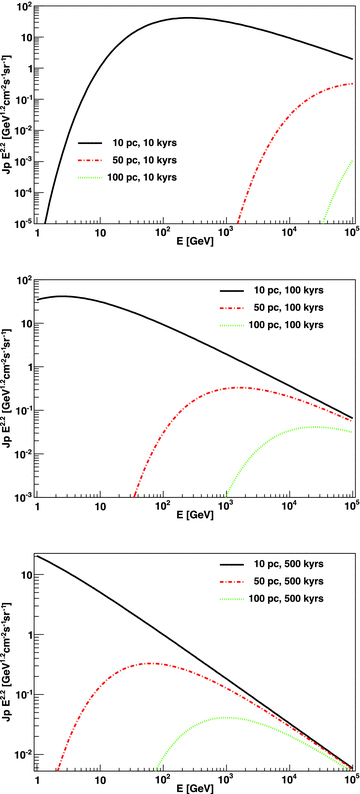
CR intensity contribution for injection at different times in the starburst history, and at different distances from the test point. Times considered are, from top to bottom, 10⁴, 10⁵ and 5 × 10⁵ yr.

Open in new tabDownload slide

Fig. 2 can be understood assuming that ⁠, and thus, from equation (7) and using the adopted parameters, one gets the diffusion radius as R_dif∼ 12 pc (E/10 GeV)^1/4(t/10⁵ yr)^1/2. We see that only high-energy particles diffuse away fast enough to reach distant regions. We also note that the ages of the accelerators we (purposefully) choose are reflected in low individual contributions to the CR intensity. They have, however, a varying E-dependent importance of which injectors are the dominant contributors.

This effect is more clearly seen in Fig. 3, in which we plot the ratio of the CR intensity as a function of energy, between an accelerator that injected particles 10⁴ and 10⁵ yr ago (top), and between 10⁴ and 5 × 10⁵ yr ago (bottom). At low energies and distances, the contribution of the older accelerator dominates that of the younger one. At 10 GeV, for instance, the diffusion radius of the 10⁴ yr old accelerator is ∼4 pc; whereas it is ∼12 pc for the 10⁵ yr old one. Then, at 10 pc, the older accelerator dominates. At higher energies, the diffusion radius of the 10⁴ yr old accelerator is larger than the test point considered and starts dominating. These results are consistent with the study by Aharonian & Atoyan (1996), and are just put here in the context of injection ages that are much larger than those typically considered for a single source (e.g. when studying the interaction of such CRs with the surrounding molecular gas, like in mid-age supernova remnants).

Figure 3

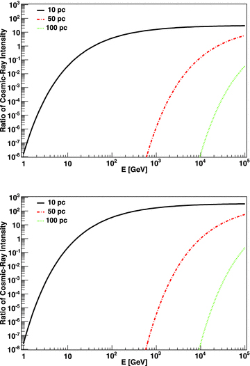
Ratio of the CR intensity as a function of the energy between a young and an old accelerator, i.e. one that injected particles at the earlier times of 10⁴ and 10⁵ yr (top), and 10⁴ and 5 × 10⁵ yr (bottom), for the three selected distances to the test point.

Open in new tabDownload slide

2.2 Homogeneous starbursts at constant explosion rate

Taking into account the individual contributions, we start by supposing that the starburst is a sphere (e.g. with a radius of 300 pc) and has experienced a constant SN explosion rate (e.g. of 0.1 SN yr⁻¹) during the recent history (e.g. during the last 1 × 10⁶ yr). With the previous values, we have a volume-average number of explosions (generically called accelerators or injectors) equal to ∼9 × 10⁻⁴ pc⁻³. In accordance with the approach described above, the total CR distribution is

9

where f_n is the individual CR contribution. In this example, then, we numerically consider 10⁵ individual solutions to equation (5). For this purpose we developed a numerical scheme that solves the diffusion-loss equation for each injector, under the assumption that the CR source is impulsive if the time that has passed since its appearance is larger than the adopted regime break of 10⁴ yr and continuous otherwise, and sums them all up. We randomize via Monte Carlo (MC) the position and time of appearance of each accelerator (with the specified mean explosion rate), as well as the individual parameters, in particular, the energy input is randomized in the range erg for an impulsive case, and in the range erg s⁻¹ for a continuous case. We again assume that the diffusion coefficient at 10 GeV is 10²⁶ cm² s⁻¹ and δ= 0.5 in a medium of density n= 35 cm⁻³. Each source spectrum was taken to have a slope of 2.2, but we also considered the case where the slope was randomly selected in an interval around this value.

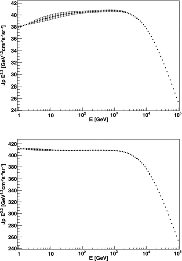
Our results verify the approximate isotropy of the CR distribution. Unless we are interested in an analysis test point that is too close to a recent accelerator location, we find that the CR distribution is homogeneous. For example, in the top panel of Fig. 4 we show an example of the results for antipodal positions in azimuth and zenith angle, at a distance of 100 pc from the centre of the starburst. Our results also show that the CR intensity is a function of starburst centre distance, being smaller the farther away from it we locate the test region. This is the result of a finite-size starburst sphere and appears as a reflection of the fact that test regions closer to the limit of the star formation environment lack the contributions of individual accelerators located beyond this distance. This is shown in the bottom panel of Fig. 4, for test positions located at different distances from the centre of the starburst. In configurations such as this, namely a starburst sphere with a limited size, the difference between the CR spectrum at the centre and its boundary can reach up to a factor of 2. This is usually neglected in the models published in the literature (see the introduction).

Figure 4

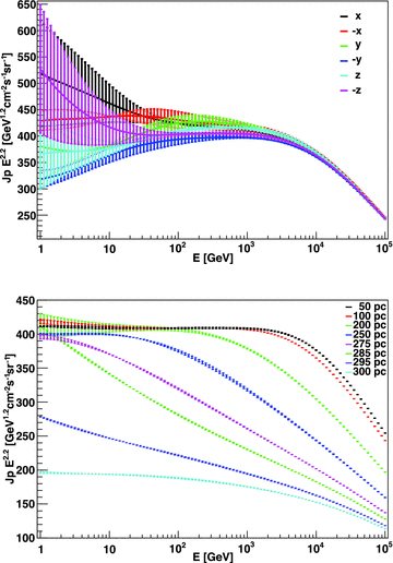
Top: CR intensity for antipodal positions in azimuth and zenith angle, all at a distance of 100 pc from the centre of the starburst. Errors result from a small number of simulations (six realizations only) and are shown merely for illustration. The larger the number of simulations, the closer all curves are to one another. For the sake of clarity of presentation, the (ordinate) flux was multiplied by the factor E^2.2. Bottom: CR intensity for test region positions located at different distances from the centre of the starburst.

Open in new tabDownload slide

We compute the CR intensity also as a function of time from the beginning of the burst, and an example is shown in Fig. 5. There we show the CR intensity in the starburst region at 50 pc from the centre at different times, from 5000 (bottom curve) to 10⁷ yr. We note that as long as the starburst is ongoing, the CR intensity increases at all energies. Although the rate of increase of the CR intensity slows down after a few hundred thousand years, it only attains a steady state after a few million years. For ∼10⁷ yr, the CR intensity in Fig. 5 would overlap with the curve corresponding to 10⁶ yr. It is then important to know the age of the starburst when detailed models are constructed, at least for ages up to yr. The latter actually depends on how dense the starburst is, in other words, how the age of the starburst compares with ⁠.

Figure 5

CR intensity in the starburst region, at 50 pc from the centre and at different times, from 5000 (bottom curve) to 10⁷ yr. The curve for 10⁷ yr overlaps the one for 10⁶ yr. Errors are derived as the standard deviation for each case after hundreds of MC realizations.

Open in new tabDownload slide

In our current setting and for our assumed explosion rate, we have about ∼500 accelerators exploding over the starburst age at positions within 50 pc of any location of interest (except of course those positions located at the boundary of the starburst). These accelerators provide more than 97 per cent of the CR intensity at each point. This can be seen in the example of Fig. 6, where we plot the percentage of the total (integral) CR intensity contributed by individual accelerators as a function of their distance to the test point. The contributions of individual accelerators surrounding a test position at 100 pc from the centre are shown in the bottom panel of Fig. 6.

Figure 6

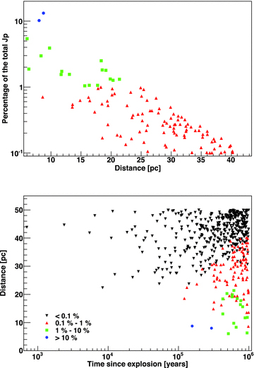
Top: example of CR intensity contributions as a function of distance (around 50 pc from the test position, located at 100 pc from the centre of the starburst). The blue points show accelerators that contribute more than 10 per cent of the total flux, green denotes those contributing between 1 and 10 per cent and red those contributing between 0.1 and 1 per cent. Bottom: contributions of individual accelerators surrounding a test position at 100 pc from the centre; the black dots represent contributions of less than 0.1 per cent.

Open in new tabDownload slide

2.3 Varying the diffusion coefficient

Since the diffusion coefficient is actually unknown, we have also considered the effect of a faster diffusion (a larger D_{10 GeV}, leading to a shorter time-scale for diffusion of particles). As expected, the larger the D, the smaller is the CR population at higher energies. This is exemplified at a fixed distance (50 pc) from the centre of the starburst in Fig. 7. We also plot in the bottom panel of that figure the CR intensity for test positions located at different distances from the centre of the starburst, as in Fig. 4 but for D_{10 GeV}= 10²⁷ cm² s⁻¹. These figures lead to the following conclusion: it is interesting to note that the discovery of a hard spectrum up to the highest energies would favour a small diffusion coefficient in starburst galaxies.

Figure 7

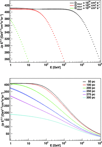
Top: example of CR intensity at 50 pc from the centre as a function of D. Bottom: CR intensity for test positions located at different distances from the centre of the starburst, as in Fig. 4 but for D_10GeV= 10²⁷ cm² s⁻¹.

Open in new tabDownload slide

If one considers that gamma-rays are ∼10 times less energetic than the protons that generated them, differences in the gamma-ray spectrum at, say, 1–10 TeV should be clear despite possible degeneracies introduced by differences in modelling the injection or the size of the emitting region. Generally, the flatter the spectrum at the highest energies, the better is the case for a small D. However, it is difficult to determine such changes from the analysis of current measurements. Fig. 7 shows that for D_{10 GeV}= 10²⁷ cm² s⁻¹, the E^2.2J_p flux drops by a factor of 4 over an energy range of 1000, between E_p= 10 GeV and 10 TeV (roughly corresponding to E_γ∼ 1 GeV and 1 TeV). That translates to a spectral steepening of 0.2. This measurement is particularly suitable for the forthcoming Cherenkov Telescope Array (Actis et al. 2011), which should provide a detailed gamma-ray spectrum of nearby starburst galaxies from a few tens of GeV up to 100 TeV.

2.4 Stability of results

We have tested many realizations of the set of positions where the injectors are located along the lifetime of the starburst, and the only visible difference is set by the proximity to the test point of the nearest injector. This produces differences especially at low energies, given the results commented in the previous section, but not an appreciable difference at energies beyond 100 GeV. At high energies, since the diffusion scales grow, the contribution is about the same irrespective of the distribution (high-energy protons diffuse significantly away from accelerators). As an example of the stability of the results obtained out of a given realization we plot the CR intensity at 50 pc from the starburst centre for accelerator appearance rates of 0.01 and 0.1 (see Fig. 8). The errors are the derived standard deviation after thousands of MC realizations. Points at higher energies show barely any error.

Figure 8

CR intensity at 50 pc from the starburst centre for accelerator appearance rates of 0.01 (top) and 0.1 (bottom) and derived standard deviation after thousands of MC realizations.

Open in new tabDownload slide

We ran two additional tests. The first one is on the influence of a fixed value of the slope of the CR injection for all accelerators instead of a variable one, which we have chosen in the range 2.0–2.4 (see, e.g., Bell, Schure & Reville 2011). That is, in the second case each injector has a different (randomly assigned) slope on its CR spectral injection. The results are depicted in Fig. 9 where we see that the change is visible especially at high energies, where it can reach up to ∼40 per cent due to the influence of harder injectors.

Figure 9

Ratio of CR intensity for configurations allowing a variable [2.0–2.4] and fixed [2.2] slope of the injection spectra, and its derived standard deviation after thousands of MC realizations of the accelerator positions and times of their appearance. Bottom: ratio for CR intensity with different regime breaks. In both cases the test point was chosen at 50 pc from the centre of the starburst, as an example.

Open in new tabDownload slide

We have also tested the influence of a different cut between the impulsive and continuous assumptions for the accelerators (i.e. a different regime break), by studying the stability of the results for breaks at 50 000 and 100 000 yr. The second panel of Fig. 9 shows the ratio for the CR intensity with different regime breaks with that considered earlier at a test point 50 pc away from the starburst centre. The larger the regime break, the more accelerators are considered continuous injectors. This explains why the CR intensity is smaller the larger the break point: the higher the energy, the shorter is the time a particle takes to reach the test point in the case of a continuous accelerator, producing a difference of up to a few per cent in the case of a 50 000 yr break.

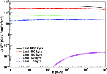
2.5 Terminated star formation burst

To exemplify the CR decay, we analyse the situation in which the star formation is exhausted in the whole starburst. Fig. 10 shows how fast the CR spectrum dies out when the star formation stops as a function of time from the end of the burst. It is interesting to note that the CR spectrum, even in cases in which the last accelerator appeared 5 × 10⁵ yr ago, is only a factor of 2 less than what it would be under a continuous star-forming process. The time-scale for decay in this model is of the order of ⁠, as might be expected if pion production is the only loss. The decay of the CR spectrum is slow as shown in the bottom panel of Fig. 10. We obtained similar results also for the case in which there is a remaining residual star formation only in the central part of the original region.

Figure 10

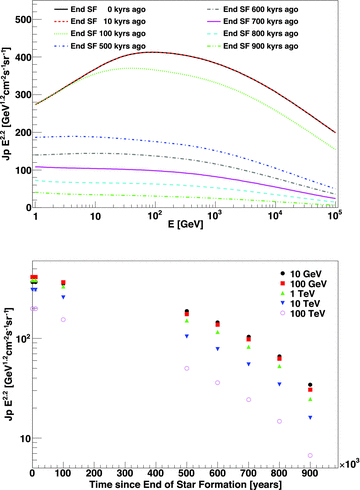
Top: CR spectrum today for different times at which the star formation is exhausted. Bottom: decay of the CR intensity as a function of time and energy.

Open in new tabDownload slide

3 THE CASE OF NGC 253

We now consider a core-enhanced SFR distribution where the starburst geometry is divided into a central sphere (or innermost starburst, ISB), in which the star formation is maximal, and a surrounding disc. Such a situation is typical in starburst galaxies, and has been considered, for instance, for NGC 253, where infrared (IR), millimetre and centimetre observations show that the central region dominates ongoing star formation (e.g. Ulvestad & Antonucci 1997; Ulvestad 2000). Current estimates of the gas mass in the central 20–50 arcsec region range from 2.5 × 10⁷ (Harrison, Henkel & Russel 1999) to (Houghton et al. 1997); see Bradford et al. (2003), Sorai et al. (2000) and Engelbracht et al. (1998). We also note that a detailed numerical treatment of the steady-state distribution of CR electrons and protons in NGC 253 was recently carried out by Paglione et al. (1996), Domingo-Santamaría & Torres (2005) and Rephaeli et al. (2010). In the latter case, their modified galprop code follows the evolution of particle energy and spatial distribution functions in the context of a diffusion–convection model. No time-dependent analysis of the contribution of individual accelerators is included.

Here, following Domingo-Santamaría & Torres (2005) we will assume, in agreement with the mentioned measurements, that within the central 200 pc (100 pc radius), a disc of 70 pc hosts 3 × 10⁷ M_⊙ of molecular mass, uniformly distributed, with a density of ∼600 cm⁻³. In this region, the SN explosion rate is taken as 0.08 yr⁻¹. We have also considered a lower value for the accelerator appearance in the core (0.02 yr⁻¹). This is motivated by the relationship between SN rate and IR luminosity (Lacki et al. 2011) and also by the fact that Melo et al. (2002) indicate that 50 per cent of the IR luminosity (and 70 per cent of the star formation) is in the starburst and 30 per cent of the IR and star formation is in the surrounding disc. Williams & Bower (2010) also find that about half of the GHz radio emission is extended (from the disc) and half comes from the starburst core, which, to the extent that the far-IR radio correlation holds, suggests roughly equal SFRs in the starburst and the surrounding disc.

Additional mass with an average density of ∼50 cm⁻³ is assumed to be in the central kpc outside the innermost region, but subject to a smaller injector rate of 0.01 yr⁻¹, or ∼ 10 per cent of that found in the most powerful nucleus (Ulvestad 2000). We assume that each injector accelerates CRs with a spectral slope between 2.2 and 2.4, randomly assigned.

Fig. 11 shows the result for the CR distribution at high energies and at different distances from the centre of NGC 253, within and outside the ISB region with the highest accelerator appearance rate. Results for different accelerator appearance rates in the ISB are shown. Each value of N_p is obtained by summing up all contributions coming from accelerators located in the ISB as well as those located in the disc. The top panel also shows the average CR distribution obtained by Domingo-Santamaría & Torres (2005), based on the treatment described in the introduction. The impact of a core-enhanced rate distribution is evident, with a significant change, of more than an order of magnitude at 1 TeV, in the CR density when the distance is increased from 50 to 200 pc from the centre (i.e. from within to outside the innermost nucleus). There is in addition a significant change in the CR distribution further outside of the nucleus; the plot shows it for distances from 200 to 400 pc along the surrounding disc. The bottom panel of Fig. 11 shows the ratio between the CR distribution in the sphere and that at different distances from the centre as a function of energy. It can be seen again that large values of the ratio are obtained, even for a smaller difference between the rates of the ISB and that of the surrounding disc. Thus, one-zone models are a rough approximation to this situation.

Figure 11

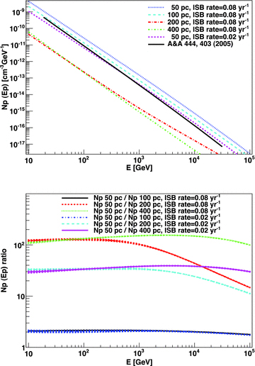
Model for the CR distribution in NGC 253. Shown in the upper panel are proton spectra at high energies, and at different distances from the galaxy centre, along the plane. The bottom panel shows the ratio between the CR distribution at 50 pc in the ISB and that at different distances, within the central core and along the disc, as a function of energy. Two different accelerator appearance rates are considered.

Open in new tabDownload slide

4 CONCLUDING REMARKS

The results presented in this paper are based on a step-by-step approach for the computation of the build-up of the CR spectrum in star-forming environments: the respective contribution of each accelerator injecting CRs over the history of the star-forming region is individually accounted for. The total spectrum is then obtained by summing up all individual contributions, taking into account an energy-, time- and space-dependent propagation of the CRs in the starburst environment. Even with the caveat of not yet considering outflows, the total spectrum shows two features that are found from gamma-ray observations of starburst galaxies: (1) that the average photon index of the current CR spectrum in starbursts is hard, even though the CR spectrum of the individual injectors suffers significant steepening due to their propagation, and (2) put in context the fact that the integrated CR spectrum (and its gamma-ray yield) scales linearly with the SFR. The latter can also be considered an observed fact given that the gamma-ray luminosity of nearby star-forming galaxies seems to scale linearly with the radio continuum and IR luminosity, both established tracers of star formation. Our simulations show that the discovery of a hard spectrum up to the highest energies would favour a small diffusion coefficient. Our results also prove that in the calorimetric limit (with no CR advection), homogeneity is reached (typically within 20 per cent) across the whole starburst region. However, values of centre-to-edge intensity ratios can amount to a factor of several. Differences between the common homogeneous assumption for the CR distribution and our models are larger in the case of two-zone geometries, such as a central nucleus with a surrounding disc. We have also found that the decay of the CR density after the starburst process is terminated is slow, and even approximately 1 Myr after the burst ends (for a gas density of 35 cm⁻³) it may still be within an order of magnitude of its peak value.

This work was supported by the grants AYA2009-07391 and SGR2009-811, as well as the Formosa programme TW2010005 and iLINK programme 2011-0303. AC is a member of the Carrera del Investigador Científico of CONICET, Argentina. BL is supported by a Jansky fellowship from the NRAO. NRAO is operated by Associated Universities, Inc., under cooperative agreement with the National Science Foundation. We thank Ana Y. Rodriguez-Marrero, A. Caliandro, G. Pedaletti and O. Reimer for discussions.

REFERENCES