


Abstract
The source counts of galaxies discovered at submillimetre and millimetre wavelengths provide important information on the evolution of infrared-bright galaxies. We combine the data from six blank-field surveys carried out at 1.1 mm with AzTEC, totalling 1.6 deg2 in area with root-mean-square depths ranging from 0.4 to 1.7 mJy, and derive the strongest constraints to date on the 1.1 mm source counts at flux densities S1100= 1–12 mJy. Using additional data from the AzTEC Cluster Environment Survey to extend the counts to S1100∼ 20 mJy, we see tentative evidence for an enhancement relative to the exponential drop in the counts at S1100∼ 13 mJy and a smooth connection to the bright source counts at >20 mJy measured by the South Pole Telescope; this excess may be due to strong-lensing effects. We compare these counts to predictions from several semi-analytical and phenomenological models and find that for most the agreement is quite good at flux densities ≳ 4 mJy; however, we find significant discrepancies (≳ 3σ) between the models and the observed 1.1-mm counts at lower flux densities, and none of them is consistent with the observed turnover in the Euclidean-normalized counts at S1100≲ 2 mJy. Our new results therefore may require modifications to existing evolutionary models for low-luminosity galaxies. Alternatively, the discrepancy between the measured counts at the faint end and predictions from phenomenological models could arise from limited knowledge of the spectral energy distributions of faint galaxies in the local Universe.
1 INTRODUCTION
Understanding how star formation evolved over the history of the Universe is one of the main goals of extragalactic astronomy today. Dust-obscured star formation is known to be a major contributor to the cosmic star formation history, as the cosmic infrared background (CIRB) accounts for ∼50 per cent of the total extragalactic background light (Puget et al. 1996). Galaxies that are selected by their redshifted, thermal dust emission at submillimetre (submm) and millimetre (mm) wavelengths, hereafter SMGs (Smail et al. 1997; Barger et al. 1998; Hughes et al. 1998), are therefore thought to play a major role in the rapid build-up of the stellar populations within massive systems.
SMGs are predominantly high-redshift (z≳ 1), dust-obscured galaxies whose far-infrared (FIR) luminosities (LFIR≳ 1012 L⊙) imply high star formation rates (SFRs) of ≳100 M⊙ yr−1; it is therefore generally believed that SMGs are observed during an important starburst or active phase in their evolution, en route to becoming massive elliptical galaxies at z= 0 (see review by Blain et al. 2002). Since the rest-frame peak of the spectral energy distribution (SED) at  m is increasingly redshifted into the submm/mm observing bands with increasing distance, there is a strong negative k-correction for surveys carried out at
  m. SMGs over a wide range in redshift (1 ≲z≲ 10) are thus readily detected in deep, wide area surveys at these wavelengths, and consequently, their basic statistical properties – such as their number density, redshift distribution, and clustering strength – hold important clues to how the most massive galaxies assemble over time.
The source counts of SMGs as a function of flux density provide strong constraints for modelling the formation and evolution of IR-bright galaxies. There are two different methods for incorporating such constraints into models. The first method, often referred to as semi-analytical or forward evolution models, typically uses numerical simulations to describe the gravitational collapse of dark matter, combined with semi-analytical recipes to govern the evolution of baryonic processes within a galaxy, with some models including complex processes such as feedback from supernovae (SNe) and/or active galactic nuclei (AGNs) (e.g. Granato et al. 2004; Baugh et al. 2005; Lacey et al. 2010). The second type are phenomenological models – or parametric backward evolution models – which make use of observational constraints (such as source counts and redshift distributions for galaxy populations selected at different wavelengths) to derive a model for the evolution of the luminosity function of galaxies, considering different populations of galaxies and SEDs (e.g. Pearson & Khan 2009; Rowan-Robinson 2009; Valiante et al. 2009; Béthermin et al. 2011). The source counts of SMGs measured from both long-wavelength ( m) ground-based surveys (e.g. Coppin et al. 2006; Bertoldi et al. 2007; Weiß et al. 2009; Austermann et al. 2010; Vieira et al. 2010; Marriage et al. 2011) and shorter wavelength (
 m) surveys from balloon- or space-based observatories (e.g. Patanchon et al. 2009; Clements et al. 2010; Oliver et al. 2010) require strong evolution in the properties of IR-bright galaxies.
In many ways, surveys at  m from the Spitzer Space Telescope and the Herschel Space Observatory have surpassed those at longer wavelengths in terms of statistical power. The large areas combined with the significant depths of these surveys make them sensitive to a much broader range of galaxy types, whereas existing surveys at longer wavelengths are limited to only the most luminous systems. However, due to well-known selection effects (e.g. Blain et al. 2002), longer wavelength data probe, on average, higher redshift and/or colder galaxies, both of which are important components for understanding galaxy evolution. Several groups (e.g. Devlin et al. 2009; Chary & Pope 2010) have shown that Spitzer/MIPS 24
  m selected galaxies, which are predominately at z≲ 1.5, account for 55–95 per cent of the CIRB at 70–500
  m. However, these sources account for only ∼30 per cent of the CIRB at λ= 1 mm (Scott et al. 2010; Penner et al. 2011). This suggests that galaxies selected at
  m, even in the deepest surveys, largely miss dust-obscured star formation activity at z≳ 1.5. The study of SMGs at
  m is thus essential to improving our understanding of the bulk of star formation taking place at higher redshifts.
There have been several deep (in some cases, confusion-limited) surveys carried out at 1.1 mm with AzTEC on the James Clerk Maxwell Telescope (JCMT) and the Atacama Submillimeter Telescope Experiment (ASTE; Ezawa et al. 2004, 2008). In this paper, we combine all previously published blank-field survey data taken with AzTEC in order to determine the strongest constraints to date on the number density of SMGs detected at  m. Given the large total area of these combined fields, the uncertainty in the measured source counts from cosmic variance is very low. The 1.1 mm source counts presented here thus provide important information on the highest redshift, IR-bright galaxies, and can be used for improving models of galaxy evolution.
This paper is organized as follows. In Section 2, we provide a summary of the blank-field surveys used to derive the combined-field source counts. In Section 3, we describe the bootstrap sampling method used to derive the 1.1 mm source counts, and we discuss how we incorporate systematic uncertainties from cosmic variance and flux calibration into our total error estimates. In Section 4, we discuss estimates of the source counts at very high flux densities determined from the South Pole Telescope (SPT) and other AzTEC surveys; we compare the combined-field 1.1 mm source counts with predictions from current galaxy evolution models in Section 5; we discuss these results in Section 6. We summarize this work in Section 7.
2 SUMMARY OF AzTEC BLANK-FIELD SURVEYS
We select the six individual blank-field surveys carried out with AzTEC (Wilson et al. 2008) on JCMT and ASTE from 2005 to 2008; each is briefly described below. Table 1 lists these fields, the telescope used, map area, depth, and number of SMGs detected in each. Note that we do not use AzTEC surveys of fields towards known overdensities, such as the AzTEC/ASTE map of the SSA-22 field towards a protocluster at z= 3.1 (Tamura et al. 2009), and the AzTEC/JCMT map of the MS-0451.6-0305 cluster at z= 0.54 (Wardlow et al. 2010). Our intent is to produce the strongest constraints on the unbiased 1.1 mm source counts, extracted from ‘blank’ fields with no prior known over- or under-densities.
Summary of AzTEC blank-field surveys. The columns are: (1) the field name; (2) the telescope used for the survey; (3) the area of the survey within the 50 per cent uniform coverage region (see Section 2); (4) the range of rms noise within the 50 per cent uniform coverage region; (5) the number of SMGs detected in the 50 per cent uniform coverage region whose probability of de-boosting to <0 mJy is P(S < 0) ≤ 0.20 for sources detected in JCMT surveys and P(S < 0) ≤ 0.05 for sources detected in ASTE surveys (see Section 3.1); (6) the root cosmic variance for the survey, following the estimate of Moster et al. (2011) (see Section 3.3); and (7) the previous paper describing the survey.
| Field | Telescope | A (deg2) | σrms (mJy beam−1) | N | σgg | References |
| GOODS-N | JCMT | 0.08 | 1.2–1.7 | 50 | 0.125 | Perera et al. (2008) |
| LH | JCMT | 0.30 | 1.1–1.6 | 180 | 0.088 | Austermann et al. (2010) |
| GOODS-S | ASTE | 0.08 | 0.5–0.8 | 66 | 0.129 | Scott et al. (2010) |
| ADF-S | ASTE | 0.20 | 0.4–0.6 | 279 | 0.086 | Hatsukade et al. (2011) |
| SXDF | ASTE | 0.21 | 0.5–0.7 | 271 | 0.098 | Hatsukade et al. (2011) |
| COSMOS | ASTE | 0.72 | 1.2–1.7 | 230 | 0.065 | Aretxaga et al. (2011) |
| All | 1.60 | 0.4–1.7 | 1076 | 0.039 |
AzTEC map sensitivities tend to decrease from the map centre to the edges due to the scanning strategies typically employed. For uniformity, we consider the ‘50 per cent coverage region’ for all fields, which encompasses all pixels in a map for which the coverage (i.e. the inverse variance weight) is ≥50 per cent of the maximum coverage. This ensures that we are only considering regions of the maps that are well sampled by several detectors, with good cross-linking, and where the noise properties are uniform. The area and the range of 1σ root-mean-square (rms) depth for each field are listed in Table 1. The combined fields result in a total area of 1.6 deg2 mapped to 1σ= 0.4–1.7 mJy beam−1. The resolutions of the JCMT and ASTE data at λ= 1.1 mm are θ= 18 and 28 arcsec (full width at half-maximum), respectively.
All of the AzTEC data were reduced using the standard customised data reduction pipeline in IDL; this is described in detail in Scott et al. (2008), so we do not describe it here. We recently derived an improvement in our estimated transfer function for point sources, as discussed in Downes et al. (2011). This typically results in an increase of 10–30 per cent in the measured flux densities of point sources detected in the maps. This also increases the noise in the maps by roughly the same amount, such that the number of SMGs detected based on a signal-to-noise ratio threshold does not change significantly. Downes et al. (2011) provide revised source lists for the majority of previously published catalogues. This will also result in a shift of the source counts published prior to this correction, which affects all of the fields considered here with the exception of COSMOS (Aretxaga et al. 2011); however, the effect on the source counts is smaller, since the higher noise levels make flux boosting effects stronger (see Austermann et al. 2009, 2010), and in turn, the de-boosting corrections are larger.
AzTEC/JCMT survey of the Great Observatories Origins Deep-North field. The AzTEC survey of the Great Observatories Origins Deep-North (GOODS-N) field was carried out during the 2005 to 2006 observing campaign on JCMT and is presented in Perera et al. (2008). GOODS-N is one of the most studied fields at all wavelengths, and much work has been done to identify the multiwavelength counterparts to the SMGs discovered in the AzTEC survey (Chapin et al. 2009b). These data have therefore been used extensively to characterize the redshift distribution, AGN fraction, etc., of mm-selected sources (Yun et al. 2012; Johnson et al., in preparation). The revised catalogue for this survey, which incorporates the improved transfer function estimate, is presented in Downes et al. (2011).
AzTEC/JCMT survey of the Lockman Hole field. A region in the Lockman Hole (LH) field was observed by AzTEC on JCMT during the 2005 to 2006 observing campaign as part of the SCUBA HAlf-Degree Extragalactic Survey (SHADES) project and is described in Austermann et al. (2010). SHADES consists of two discontiguous fields: the LH, and the Subaru/XMM–Newton Deep Field (SXDF). We do not use the AzTEC/JCMT map of SXDF in our combined source counts analysis, since it largely overlaps with the ASTE survey of the same field (see below) and is considerably shallower. As with GOODS-N, the revised source catalogue for LH is presented in Downes et al. (2011).
AzTEC/ASTE survey of the GOODS-S field. The AzTEC survey of the GOODS-South (GOODS-S) field was carried out on the ASTE telescope during the 2007 observing run and is presented in Scott et al. (2010). As with GOODS-N, extensive efforts to identify multiwavelength counterparts for AzTEC/GOODS-S SMGs and to derive the redshift distribution, SFR, and stellar mass properties of SMGs from these data have already been carried out (Yun et al. 2012; Johnson et al., in preparation). The revised catalogue using the new transfer function estimate is given in Downes et al. (2011). In general, the fractional increase in the measured source flux densities and map noise is lower for the ASTE maps compared to the JCMT maps.
AzTEC/ASTE survey of the Akari Deep Field-South. The AzTEC map of the Akari Deep Field-South (ADF-S) was built up over the 2007 and 2008 observing runs on ASTE and is discussed in Hatsukade et al. (2011). This is the deepest map used in our analysis and therefore puts strong constraints on the faint end of the source counts.
AzTEC/ASTE survey of SXDF. The AzTEC survey of SXDF carried out on ASTE during 2007 and 2008 is a slightly smaller but considerably deeper survey than the AzTEC SXDF map taken as part of the SHADES project on JCMT. The source counts from this survey are presented in Hatsukade et al. (2011), and, similar to ADF-S, these data provide strong constraints on the faint end of the source counts.
AzTEC/ASTE survey of the COSMOS field. The largest survey used in our combined source counts analysis is the AzTEC survey of the COSMOS field, carried out during the 2008 observing campaign on ASTE (Aretxaga et al. 2011). This survey almost completely encompasses the smaller, shallower AzTEC map taken with JCMT in 2005 to 2006 (Scott et al. 2008), so we do not use the latter in our analysis. Being a factor of >2 larger than the other surveys considered here, this field provides the strongest constraints on the bright end of the 1.1 mm source counts. The map used in our analysis here is the same as that presented in Aretxaga et al. (2011), which used the improved transfer function of Downes et al. (2011). Like the two GOODS fields, COSMOS is one of the best studied regions at all wavelengths, and the SMGs detected in this field have been used to study the properties of the SMG population at complementary wavelengths (Johnson et al., in preparation).
3 1.1 mm SOURCE COUNTS FROM COMBINED BLANK FIELDS
3.1 Bootstrap sampling method
To derive the 1.1 mm source counts, we adopt the standard bootstrap sampling method that has been used extensively in the past for extracting the counts from AzTEC surveys. This method, first introduced by Coppin et al. (2006) and further developed for use with AzTEC data, is described in great detail in Austermann et al. (2009) and Austermann et al. (2010), and we briefly summarize it here.
Using the source catalogue from one or more surveys and assuming a prior distribution for the source counts based on the best-fitting Schechter function to the COSMOS counts (Aretxaga et al. 2011), we construct posterior flux distributions (PFDs) for each source that are sampled at random in order to determine intrinsic flux densities for the sources in the catalogue; these are then binned to derive the differential and integrated source counts. Only sources that pass the ‘null threshold’ test are sampled in order to avoid including a large number of false positives, that is, we only sample sources for which the probability that their intrinsic flux is less than zero is P(S < 0) ≤ 0.20 for sources detected in JCMT surveys and P(S < 0) ≤ 0.05 for sources detected in ASTE surveys. The more stringent limit for the ASTE data is imposed due to larger systematics from confusion in estimating the PFDs (see discussion in Scott et al. 2010). This process is repeated 20 000 times in order to sufficiently sample the source count probability distribution, and the mean and 68.3 per cent confidence interval for the counts in evenly spaced, 1-mJy-wide flux bins are computed from these iterations, giving the raw source counts. These raw counts are then corrected for incompleteness, which is estimated through simulation by calculating the recovery rate as a function of flux density for simulated sources injected (one at a time) into the map (see e.g. Scott et al. 2010). We use the same source detection algorithm and null threshold test on these simulated sources as that used for the real catalogues to quantify the survey completeness. These corrected counts are then divided by the survey area to determine the differential (dN/dS) and integral [N(> S)] source counts.
We compute the counts only for flux densities ≥ 1 mJy; at lower flux densities, completeness is too low (≲10 per cent) and difficult to estimate. While the completeness in our three shallowest fields (GOODS-N, LH and COSMOS) is <5 per cent at 1 mJy, the deeper surveys are 15–30 per cent complete at this same flux level, ensuring that the low-flux end of the counts will not be subject to significant errors from biases in our completeness estimate.
Another common method for extracting source counts from this type of low-resolution, confusion-limited survey is the probability of deflection, or ‘P(D)’, approach, and it has been commonly employed for extracting counts from recent BLAST and Herschel-SPIRE surveys (e.g. Patanchon et al. 2009; Glenn et al. 2010). The P(D) technique avoids certain biases inherent in the bootstrap sampling method – namely, the bias to the counts from the assumed prior distribution, and biases from the assumption that each detected ‘source’ really represents the emission from a single galaxy. Also, in principle, the P(D) method allows an estimate of the source counts at fainter flux densities, below the detection limit of individual point sources. On the other hand, source counts determined from the P(D) approach must use piecewise models, where the differential counts at selected ‘nodes’ (i.e. fixed flux densities) are free parameters, and the nodes are connected by some smooth function. Such models may adequately reproduce the observed fluctuations in a map; however, they are not at all physically motivated. While increasing the resolution between nodes can reduce the model dependency of the counts, this increases the number of free parameters as well as the correlations between them. In practice, most groups limit the number of nodes so that the fitted parameters are largely uncorrelated, at the expense of making their results more model-dependent; consequently, the formal errors on the fitted parameters may not always represent the true uncertainty in the counts (see e.g. discussions in Scott et al. 2010; Glenn et al. 2010). Furthermore, while the implementation of the P(D) method is relatively straightforward when the transfer function for point sources is linear, this is not the case for our PCA-cleaned AzTEC maps (Downes et al. 2011), and the P(D) method thus becomes computationally expensive for our data. This is why we have chosen to use the bootstrap sampling method instead.
Austermann et al. (2010) demonstrated that for flux bins that are well sampled, the assumed prior used in the bootstrap sampling approach is quite weak. Furthermore, they show that biases to the counts for sparsely sampled flux bins can be effectively removed by an iterative process in which the counts extracted from the first pass are used to update the prior and PFDs for the source catalogue(s), and the bootstrap sampling method is repeated. We use this iterative process to decrease the effects of the prior on the extracted source counts. The counts from the combined blank fields change by less than 2 per cent in all flux bins after only three iterations.
We list in Table 1 the total number of sources in each field that were used to extract the counts. The counts from the combined blank fields are shown in Fig. 1 (filled circles), and are listed in Table 2, where the upper and lower error bars indicate 68.3 per cent confidence intervals. We give the correlation matrices (see appendix A in Austermann et al. 2010) for the differential and integrated source counts in Tables 3 and 4, respectively, and we list the standard deviation on the counts, σdN/dS and σN(> S), for each bin as well, from which the covariance matrices can be determined. We have made the source counts and correlation matrices available online for public use.1 Since the counts are determined from bootstrapping off the PFDs of the sources, adjacent flux bins are strongly correlated. It is therefore important to use the covariance matrix in model fitting, for example, for fitting a model prediction m to observed counts d with covariance matrix  , the χ2 metric is given by
  .
.
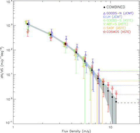
Differential source counts derived from the six blank-field surveys carried out with AzTEC on JCMT and ASTE. The counts determined from each individual field are as follows: triangles – GOODS-N; squares – LH; diamonds – GOODS-S; inverted triangles – ADF-S; circles – SXDF; stars – COSMOS. The counts derived from combining these six fields are shown as the black filled circles. The counts for the individual blank fields have been computed in slightly different flux bins for clarity in plotting. All error bars show the 68.3 per cent confidence intervals determined from the bootstrap sampling method, including uncertainties arising from cosmic variance (see Section 3.3). The uncertainty from flux calibration (Section 3.4) is not included since all fields were calibrated the same way. The shaded region highlights the 68.3 per cent confidence range on the combined counts. The horizontal lines at the bottom right-hand side indicate the survey limits for each individual field (dotted) and for the combined counts (dashed). The survey limit corresponds to the expected value for which the source counts will Poisson deviate to zero 31.7 per cent of the time, given the area of the survey(s). See the online journal for a colour version of this figure.
1.1 mm source counts derived from the combined six AzTEC blank-field surveys. The first two columns show the flux bin centres and corresponding differential source counts, while the last two columns show the flux bin minima and cumulative counts. The first set of upper and lower errors shown on the counts indicate the 68.3 per cent confidence intervals considering only statistical errors (Section 3.1). The second set of errors in parentheses show the 68.3 per cent confidence intervals when including systematic uncertainties from cosmic variance (Section 3.3) and flux calibration (Section 3.4). The bright source counts derived from ACES are also listed (see Section 4).
| Flux density (mJy) | dN/dS (mJy−1 deg−2) | Flux density (mJy) | N(> S) (deg−2) |
| Combined blank fields | |||
| 1.4 |  | 1.0 |  |
| 2.4 |  | 2.0 |  |
| 3.4 |  | 3.0 |  |
| 4.4 |  | 4.0 |  |
| 5.4 |  | 5.0 |  |
| 6.4 |  | 6.0 |  |
| 7.4 |  | 7.0 |  |
| 8.4 |  | 8.0 |  |
| 9.4 |  | 9.0 |  |
| 10.4 |  | 10.0 |  |
| 11.4 |  | 11.0 |  |
| ACES fields | |||
| 11.1 |  | 10.0 |  |
| 14.1 |  | 13.0 |  |
| 17.1 |  | 16.0 |  |
| Flux density (mJy) | dN/dS (mJy−1 deg−2) | Flux density (mJy) | N(> S) (deg−2) |
| Combined blank fields | |||
| 1.4 | | 1.0 | |
| 2.4 | | 2.0 | |
| 3.4 | | 3.0 | |
| 4.4 | | 4.0 | |
| 5.4 | | 5.0 | |
| 6.4 | | 6.0 | |
| 7.4 | | 7.0 | |
| 8.4 | | 8.0 | |
| 9.4 | | 9.0 | |
| 10.4 | | 10.0 | |
| 11.4 | | 11.0 | |
| ACES fields | |||
| 11.1 | | 10.0 | |
| 14.1 | | 13.0 | |
| 17.1 | | 16.0 | |
1.1 mm source counts derived from the combined six AzTEC blank-field surveys. The first two columns show the flux bin centres and corresponding differential source counts, while the last two columns show the flux bin minima and cumulative counts. The first set of upper and lower errors shown on the counts indicate the 68.3 per cent confidence intervals considering only statistical errors (Section 3.1). The second set of errors in parentheses show the 68.3 per cent confidence intervals when including systematic uncertainties from cosmic variance (Section 3.3) and flux calibration (Section 3.4). The bright source counts derived from ACES are also listed (see Section 4).
| Flux density (mJy) | dN/dS (mJy−1 deg−2) | Flux density (mJy) | N(> S) (deg−2) |
| Combined blank fields | |||
| 1.4 | | 1.0 | |
| 2.4 | | 2.0 | |
| 3.4 | | 3.0 | |
| 4.4 | | 4.0 | |
| 5.4 | | 5.0 | |
| 6.4 | | 6.0 | |
| 7.4 | | 7.0 | |
| 8.4 | | 8.0 | |
| 9.4 | | 9.0 | |
| 10.4 | | 10.0 | |
| 11.4 | | 11.0 | |
| ACES fields | |||
| 11.1 | | 10.0 | |
| 14.1 | | 13.0 | |
| 17.1 | | 16.0 | |
Correlation matrix for the differential counts derived from the combined AzTEC blank-field surveys. The first set shows the bin-to-bin correlations when considering only statistical errors from the bootstrap sampling method (Section 3.1); these represent the actual correlations between bins in the data themselves. The second, third and fourth sets show the correlations when systematic uncertainties from cosmic variance (Section 3.3), flux calibration (Section 3.4) and both are included, respectively. The last column in all four cases shows the standard deviation on the differential counts for each flux bin, and can be used to compute the covariance matrix from these correlations.
| Flux density (mJy) | 1.4 | 2.4 | 3.4 | 4.4 | 5.4 | 6.4 | 7.4 | 8.4 | 9.4 | 10.4 | 11.4 | σdN/dS (mJy−1 deg−2) |
| Statistical errors only | ||||||||||||
| 1.4 | 1.00 | 66 | ||||||||||
| 2.4 | 0.61 | 1.00 | 27 | |||||||||
| 3.4 | 0.21 | 0.62 | 1.00 | 14 | ||||||||
| 4.4 | 0.11 | 0.29 | 0.67 | 1.00 | 8.2 | |||||||
| 5.4 | 0.06 | 0.15 | 0.34 | 0.71 | 1.00 | 5.0 | ||||||
| 6.4 | 0.02 | 0.06 | 0.15 | 0.33 | 0.67 | 1.00 | 3.2 | |||||
| 7.4 | 0.00 | 0.01 | 0.05 | 0.13 | 0.32 | 0.72 | 1.00 | 2.1 | ||||
| 8.4 | −0.01 | −0.01 | 0.00 | 0.04 | 0.12 | 0.32 | 0.76 | 1.00 | 1.6 | |||
| 9.4 | 0.00 | −0.01 | −0.01 | 0.01 | 0.05 | 0.17 | 0.49 | 0.81 | 1.00 | 1.2 | ||
| 10.4 | 0.00 | −0.01 | −0.02 | −0.01 | 0.01 | 0.06 | 0.20 | 0.42 | 0.83 | 1.00 | 0.87 | |
| 11.4 | 0.00 | −0.01 | −0.02 | −0.01 | −0.01 | 0.01 | 0.07 | 0.20 | 0.54 | 0.85 | 1.00 | 0.70 |
| Including systematic uncertainties from cosmic variance | ||||||||||||
| 1.4 | 1.00 | 80 | ||||||||||
| 2.4 | 0.80 | 1.00 | 31 | |||||||||
| 3.4 | 0.57 | 0.79 | 1.00 | 15 | ||||||||
| 4.4 | 0.48 | 0.58 | 0.79 | 1.00 | 8.8 | |||||||
| 5.4 | 0.38 | 0.44 | 0.54 | 0.79 | 1.00 | 5.2 | ||||||
| 6.4 | 0.27 | 0.30 | 0.35 | 0.47 | 0.72 | 1.00 | 3.2 | |||||
| 7.4 | 0.19 | 0.21 | 0.22 | 0.27 | 0.40 | 0.73 | 1.00 | 2.1 | ||||
| 8.4 | 0.13 | 0.14 | 0.14 | 0.14 | 0.19 | 0.36 | 0.77 | 1.00 | 1.6 | |||
| 9.4 | 0.11 | 0.12 | 0.11 | 0.11 | 0.12 | 0.22 | 0.51 | 0.81 | 1.00 | 1.2 | ||
| 10.4 | 0.09 | 0.09 | 0.08 | 0.07 | 0.07 | 0.09 | 0.22 | 0.43 | 0.83 | 1.00 | 0.87 | |
| 11.4 | 0.07 | 0.08 | 0.07 | 0.06 | 0.05 | 0.05 | 0.09 | 0.22 | 0.55 | 0.85 | 1.00 | 0.71 |
| Including systematic uncertainties from flux calibration | ||||||||||||
| 1.4 | 1.00 | 94 | ||||||||||
| 2.4 | 0.58 | 1.00 | 27 | |||||||||
| 3.4 | 0.20 | 0.62 | 1.00 | 14 | ||||||||
| 4.4 | 0.11 | 0.27 | 0.67 | 1.00 | 9.3 | |||||||
| 5.4 | 0.05 | 0.14 | 0.33 | 0.71 | 1.00 | 6.5 | ||||||
| 6.4 | 0.02 | 0.06 | 0.16 | 0.32 | 0.68 | 1.00 | 4.0 | |||||
| 7.4 | 0.00 | 0.02 | 0.06 | 0.13 | 0.30 | 0.67 | 1.00 | 2.5 | ||||
| 8.4 | 0.00 | 0.00 | 0.01 | 0.03 | 0.11 | 0.34 | 0.83 | 1.00 | 1.7 | |||
| 9.4 | −0.01 | 0.00 | 0.00 | 0.01 | 0.04 | 0.16 | 0.46 | 0.75 | 1.00 | 1.3 | ||
| 10.4 | 0.00 | 0.01 | 0.00 | 0.00 | 0.00 | 0.04 | 0.17 | 0.42 | 0.86 | 1.00 | 0.92 | |
| 11.4 | 0.01 | 0.01 | 0.01 | 0.00 | 0.00 | 0.00 | 0.05 | 0.17 | 0.48 | 0.79 | 1.00 | 0.72 |
| Including systematic uncertainties from cosmic variance and flux calibration | ||||||||||||
| 1.4 | 1.00 | 100 | ||||||||||
| 2.4 | 0.78 | 1.00 | 32 | |||||||||
| 3.4 | 0.57 | 0.80 | 1.00 | 16 | ||||||||
| 4.4 | 0.47 | 0.58 | 0.79 | 1.00 | 9.9 | |||||||
| 5.4 | 0.38 | 0.44 | 0.55 | 0.79 | 1.00 | 6.7 | ||||||
| 6.4 | 0.26 | 0.30 | 0.34 | 0.45 | 0.73 | 1.00 | 4.0 | |||||
| 7.4 | 0.18 | 0.19 | 0.20 | 0.24 | 0.38 | 0.69 | 1.00 | 2.5 | ||||
| 8.4 | 0.13 | 0.14 | 0.14 | 0.15 | 0.21 | 0.40 | 0.85 | 1.00 | 1.7 | |||
| 9.4 | 0.12 | 0.12 | 0.12 | 0.12 | 0.14 | 0.22 | 0.46 | 0.75 | 1.00 | 1.3 | ||
| 10.4 | 0.09 | 0.10 | 0.10 | 0.09 | 0.09 | 0.11 | 0.20 | 0.46 | 0.86 | 1.00 | 0.91 | |
| 11.4 | 0.08 | 0.09 | 0.08 | 0.07 | 0.07 | 0.06 | 0.07 | 0.18 | 0.44 | 0.76 | 1.00 | 0.72 |
Correlation matrix for the cumulative counts derived from the combined AzTEC blank-field surveys. The first set shows the bin-to-bin correlations when considering only statistical errors from the bootstrap sampling method (Section 3.1); these represent the actual correlations between bins in the data themselves. The second, third and fourth sets show the correlations when systematic uncertainties from cosmic variance (Section 3.3), flux calibration (Section 3.4) and both are included, respectively. The last column in all four cases shows the standard deviation on the cumulative counts for each flux bin, and can be used to compute the covariance matrix from these correlations.
| Flux density (mJy) | 1.0 | 2.0 | 3.0 | 4.0 | 5.0 | 6.0 | 7.0 | 8.0 | 9.0 | 10.0 | 11.0 | σN(> S) (deg−2) |
| Statistical errors only | ||||||||||||
| 1.0 | 1.00 | 74 | ||||||||||
| 2.0 | 0.77 | 1.00 | 32 | |||||||||
| 3.0 | 0.47 | 0.83 | 1.00 | 17 | ||||||||
| 4.0 | 0.31 | 0.59 | 0.87 | 1.00 | 11 | |||||||
| 5.0 | 0.19 | 0.40 | 0.64 | 0.88 | 1.00 | 6.7 | ||||||
| 6.0 | 0.11 | 0.24 | 0.43 | 0.66 | 0.90 | 1.00 | 4.5 | |||||
| 7.0 | 0.06 | 0.15 | 0.28 | 0.48 | 0.72 | 0.92 | 1.00 | 3.2 | ||||
| 8.0 | 0.04 | 0.10 | 0.21 | 0.36 | 0.57 | 0.78 | 0.94 | 1.00 | 2.4 | |||
| 9.0 | 0.03 | 0.07 | 0.15 | 0.27 | 0.44 | 0.63 | 0.80 | 0.93 | 1.00 | 1.8 | ||
| 10.0 | 0.02 | 0.05 | 0.11 | 0.21 | 0.34 | 0.49 | 0.65 | 0.80 | 0.95 | 1.00 | 1.4 | |
| 11.0 | 0.02 | 0.04 | 0.08 | 0.16 | 0.26 | 0.38 | 0.52 | 0.66 | 0.84 | 0.95 | 1.00 | 1.1 |
| Including systematic uncertainties from cosmic variance | ||||||||||||
| 1.0 | 1.00 | 100 | ||||||||||
| 2.0 | 0.90 | 1.00 | 43 | |||||||||
| 3.0 | 0.74 | 0.91 | 1.00 | 21 | ||||||||
| 4.0 | 0.61 | 0.76 | 0.91 | 1.00 | 12 | |||||||
| 5.0 | 0.46 | 0.58 | 0.73 | 0.90 | 1.00 | 7.2 | ||||||
| 6.0 | 0.32 | 0.41 | 0.53 | 0.70 | 0.90 | 1.00 | 4.7 | |||||
| 7.0 | 0.23 | 0.29 | 0.38 | 0.52 | 0.73 | 0.92 | 1.00 | 3.3 | ||||
| 8.0 | 0.17 | 0.21 | 0.28 | 0.40 | 0.58 | 0.79 | 0.95 | 1.00 | 2.5 | |||
| 9.0 | 0.13 | 0.16 | 0.21 | 0.30 | 0.45 | 0.63 | 0.80 | 0.93 | 1.00 | 1.9 | ||
| 10.0 | 0.10 | 0.12 | 0.16 | 0.23 | 0.35 | 0.49 | 0.65 | 0.80 | 0.95 | 1.00 | 1.4 | |
| 11.0 | 0.07 | 0.09 | 0.13 | 0.18 | 0.27 | 0.39 | 0.51 | 0.66 | 0.83 | 0.95 | 1.00 | 1.1 |
| Including systematic uncertainties from flux calibration | ||||||||||||
| 1.0 | 1.00 | 90 | ||||||||||
| 2.0 | 0.75 | 1.00 | 35 | |||||||||
| 3.0 | 0.46 | 0.83 | 1.00 | 24 | ||||||||
| 4.0 | 0.30 | 0.59 | 0.87 | 1.00 | 18 | |||||||
| 5.0 | 0.19 | 0.39 | 0.63 | 0.88 | 1.00 | 12 | ||||||
| 6.0 | 0.11 | 0.25 | 0.43 | 0.65 | 0.89 | 1.00 | 7.1 | |||||
| 7.0 | 0.07 | 0.16 | 0.29 | 0.47 | 0.71 | 0.92 | 1.00 | 4.5 | ||||
| 8.0 | 0.05 | 0.11 | 0.21 | 0.36 | 0.57 | 0.78 | 0.94 | 1.00 | 3.1 | |||
| 9.0 | 0.03 | 0.08 | 0.16 | 0.27 | 0.42 | 0.60 | 0.78 | 0.93 | 1.00 | 2.2 | ||
| 10.0 | 0.03 | 0.07 | 0.12 | 0.20 | 0.32 | 0.47 | 0.63 | 0.80 | 0.95 | 1.00 | 1.6 | |
| 11.0 | 0.02 | 0.05 | 0.10 | 0.16 | 0.25 | 0.37 | 0.50 | 0.66 | 0.83 | 0.95 | 1.00 | 1.2 |
| Including systematic uncertainties from cosmic variance and flux calibration | ||||||||||||
| 1.0 | 1.00 | 120 | ||||||||||
| 2.0 | 0.89 | 1.00 | 45 | |||||||||
| 3.0 | 0.74 | 0.91 | 1.00 | 27 | ||||||||
| 4.0 | 0.60 | 0.75 | 0.91 | 1.00 | 19 | |||||||
| 5.0 | 0.46 | 0.57 | 0.72 | 0.90 | 1.00 | 12 | ||||||
| 6.0 | 0.32 | 0.40 | 0.52 | 0.69 | 0.90 | 1.00 | 7.2 | |||||
| 7.0 | 0.23 | 0.28 | 0.37 | 0.52 | 0.73 | 0.92 | 1.00 | 4.5 | ||||
| 8.0 | 0.18 | 0.23 | 0.29 | 0.41 | 0.59 | 0.79 | 0.94 | 1.00 | 3.1 | |||
| 9.0 | 0.14 | 0.18 | 0.23 | 0.31 | 0.46 | 0.62 | 0.78 | 0.93 | 1.00 | 2.2 | ||
| 10.0 | 0.12 | 0.14 | 0.18 | 0.24 | 0.35 | 0.48 | 0.63 | 0.81 | 0.95 | 1.00 | 1.6 | |
| 11.0 | 0.09 | 0.12 | 0.14 | 0.19 | 0.28 | 0.38 | 0.50 | 0.66 | 0.83 | 0.96 | 1.00 | 1.3 |
3.2 Effects of confusion on the extracted source counts
Using the standard definition of one source per 30 beams (e.g. Takeuchi & Ishii 2004), the confusion limit for these surveys carried out on JCMT and ASTE is Slim= 1.4 and 2.4 mJy, respectively. These correspond to the two lowest flux bins in our source counts estimate. In this section, we explore potential biases to the extracted counts due to confusion effects.
The results from these simulations are presented in Fig. 2, which shows the Euclidean-normalized differential source counts averaged over the 100 simulated maps for each field separately (top panel). The counts have been scaled arbitrarily for clarity, with the dotted curves indicating the input source distribution from equation (1). There is evidence from these simulations that confusion introduces biases to the observed source counts. This is more evident in the bottom panel of Fig. 2, which shows the fractional difference between the input and output source counts. In general, the counts at S1100≳Slim (the confusion limit) are overestimated by ∼5–30 per cent, while the counts at S1100≲Slim are underestimated by ∼10–20 per cent. However, these biases are small compared to the statistical errors on the derived counts for these individual fields; the error bars in the top panel of Fig. 2 represent the typical 68.3 per cent confidence intervals on the extracted counts for a single simulated map. Considering all simulated data sets, the extracted counts agree with the input counts within their 2σ errors >85 per cent of the time, with the exception of the COSMOS simulated fields, where the extracted counts at S1100= 1.4 mJy are always significantly underestimated. This large discrepancy between the input and output source counts in the lowest flux density bin for COSMOS is most likely due to the low – and therefore poorly measured – completeness at that flux density.
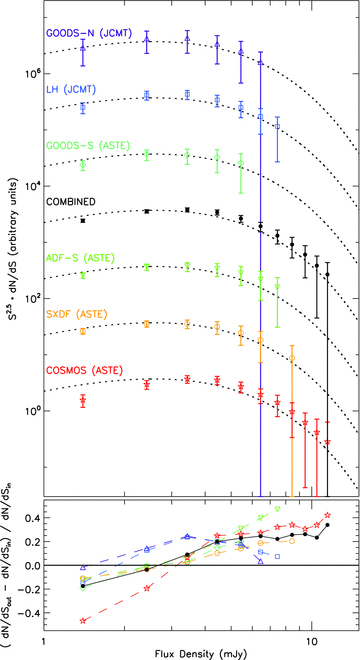
Results of simulations to test the effects of confusion on our source counts extraction, as described in Section 3.2. The top panel shows the averaged Euclidean-normalized differential source counts extracted from simulated maps for each field and for the combined fields, as labelled. For clarity, the counts have been offset by a factor of 1000, 100, 10, 0.1, 0.01 and 0.001 for the GOODS-N, LH, GOODS-S, ADF-S, SXDF and COSMOS data sets, respectively. The dotted curves show the model for the input source counts (equation 1) for comparison. The errors represent typical 68.3 per cent confidence intervals on the counts for a single simulated map, demonstrating that the biases to the extracted counts arising from confusion effects are small compared to the statistical errors. The bottom panel shows the fractional difference between the input and output source counts, using the same symbols as in the top panel. See the online journal for a colour version of this figure.
We next use the simulated maps for each field to make 100 realizations of the extracted source counts from the six fields combined. For each realization, we randomly select six simulated maps, one from each field, and carry out the joint bootstrap sampling extraction. These results are also shown in Fig. 2, and as expected, we see similar biases to the output source counts as seen in each individual field. This bias is smallest (4 per cent) for the 2.4 mJy flux density bin, which corresponds to the confusion limit for the ASTE surveys. For the lowest flux bin at 1.4 mJy, the counts are underestimated by 17 per cent, and for the bins at S1100 > 3 mJy, the counts are overestimated by 9–34 per cent. In comparison to the statistical errors, the combined-field counts derived from the simulated maps agree with the input counts within their 2σ errors > 80 per cent of the time.
3.3 Cosmic variance
The source counts determined from each individual survey are shown in Fig. 1. Given the limited area surveyed for each field, we expect to see variations in the counts from field to field owing to variations in the underlying large-scale structure (also known as ‘cosmic variance’). Furthermore, given the strong bin-to-bin correlations, the counts across all flux bins for a given survey vary in the same sense; for example, the GOODS-N counts are consistently higher than the average, while the GOODS-S counts are consistently lower. In order to assess the agreement among the counts derived from individual AzTEC fields, we must include this uncertainty from cosmic variance into the error budget.
We estimate the expected cosmic variance for each individual survey and for the combined blank fields using the prescription described in Moster et al. (2011). This estimate uses predictions of the underlying structure of cold dark matter (CDM) and the expected bias for a galaxy population – in this case, SMGs. This simple recipe depends only on the angular dimensions of the field (α1, α2), the mean redshift ( ), redshift bin size (Δz) and stellar mass (M★) of the galaxy population in question. Moster et al. (2011) have provided their software tools for calculating cosmic variance online.2
This estimate assumes rectangular geometry for the survey, which is rarely the case for our fields; however, Moster et al. (2011) show that the geometry makes little difference except where the ratio between the short and long axes of the survey is ≲ 0.2, which is not the case for any of our fields. We therefore assume angular dimensions for each field, α1 and α2, such that the product is equal to the area in the 50 per cent uniform coverage region, and the ratio approximately matches the geometry of the AzTEC map. The mean redshift, redshift bin size, and stellar mass are taken from Yun et al. (2012), who use spectroscopic and photometric redshifts for the SMGs detected in both AzTEC/GOODS fields to determine their redshift distribution, and stellar mass estimates from modelling their observed rest-frame ultraviolet and optical SEDs. Yun et al. (2012) find  , Δz= 1.5, and M★ > 1010 M⊙, where Δz and the limit on M★ encompass 75 per cent of the SMGs in that sample. The root cosmic variance, σgg, which represents the expected fractional error on the counts due to cosmic variance, is listed for each field in Table 1 and ranges from 6.5 to 12.9 per cent for the individual AzTEC fields. By combining all six fields, totalling 1.6 deg2, uncertainties due to cosmic variance are reduced to only 3.9 per cent, which is smaller than the statistical errors on the counts (≥6 per cent).
Since the uncertainty from cosmic variance is completely correlated among all flux bins, we cannot simply add σgg in quadrature with the statistical errors on the counts; instead, we must consider how including cosmic variance affects the entire covariance matrix. It is straightforward to include this effect within the framework of the bootstrap sampling method. For each of the 20 000 iterations, we generate a random number drawn from a Gaussian distribution with a mean of zero and a standard deviation of σgg, and we apply this fractional deviation to the differential source counts uniformly to all bins. The mean, 68.3 per cent confidence intervals, and the covariance matrix for the counts are then computed from the 20 000 iterations in the same manner as in the standard bootstrap method described in Section 3.1. This way we broaden the distribution in the bootstrapped counts according to the expected degree of cosmic variance and can properly trace the effects on the bin-to-bin correlations.
The 68.3 per cent confidence intervals shown by the error bars on the differential counts in Fig. 1 include the uncertainties expected from cosmic variance, for each individual field as well as the combined fields. We note that the standard deviation of the counts, σdN/dS (equal to the root of the diagonal elements of the covariance matrix), increases as expected [ ], and the bin-to-bin correlations on the counts increase substantially, as shown in Tables 3 and 4. Comparing the counts observed in each individual field when both the statistical errors and the uncertainties from cosmic variance are included, we find that they all agree quite well.
The mean redshift and interquartile range from Yun et al. (2012) which we use to estimate the cosmic variance agree very well with those derived from other spectroscopic (Chapman et al. 2003, 2005) and photometric (Aretxaga et al. 2003, 2007; Pope et al. 2005; Wardlow et al. 2011) redshift estimates, which find  and Δz= 1.1–1.8. The largest uncertainty in this estimate comes from the assumed stellar mass distribution of SMGs. Stellar mass estimates for SMGs are highly uncertain, as they depend strongly on the choice of the stellar synthesis model, star formation history, and initial mass function (IMF) – all of which are not well understood (see e.g. discussion in Michałowski et al. 2011). The stellar mass distribution of AzTEC/GOODS SMGs in Yun et al. (2012, see their fig. 8) peaks at M★∼ 1011.3 M⊙ and is broadly consistent with the mean stellar masses of SMGs estimated in other works, which range from ∼1010.8 to 1011.8 M⊙ (Dye et al. 2008; Michałowski, Hjorth & Watson 2010; Hainline et al. 2011; Wardlow et al. 2011). However, the distribution in M★ from all of these works is found to be quite broad, especially compared to the stellar mass bins used in Moster et al. (2011) for computing the galaxy bias; this is why we opt to use a lower stellar mass limit of M★ > 1010 M⊙, which includes 75 per cent of the Yun et al. (2012) sample. Increasing the lower limit on the stellar mass would increase the expected cosmic variance for these surveys, as more massive galaxies are more strongly clustered. If we instead assume M★ > 1010.5 M⊙ (as motivated to some extent by results in Michałowski et al. 2011, see their fig. 3), we would derive a root cosmic variance of 8.8–17.5 per cent for the individual AzTEC surveys and 5.3 per cent for the combined fields.
3.4 Systematic uncertainty from flux calibration
We must also consider a systematic uncertainty on the derived source counts arising from uncertainty in the absolute flux calibration of our data. For AzTEC data, we determine flux conversion factors to convert the raw detector signals to flux density units based on several calibration observations of planets taken over a wide range of atmospheric conditions (see Wilson et al. 2008, for details). While the random calibration error of an individual observation is ∼10 per cent (Scott et al. 2010), co-added AzTEC maps are each built from 46 to 325 observations, and the error on our measured source flux densities integrates down to 0.3 per cent when all observations, and all fields, are considered. However, for all of these data we use the same flux calibrators, Uranus and Neptune, which have an absolute uncertainty on their flux densities of σcal= 5 per cent (Griffin & Orton 1993). This is a systematic uncertainty in the flux scale of our maps that is completely correlated among all AzTEC data and therefore propagates into the source counts.
As with cosmic variance, we incorporate this calibration uncertainty into the bootstrap sampling method. For each of the 20 000 iterations, we generate a random number drawn from a Gaussian distribution with a mean of zero and a standard deviation of σcal. We then modify the PFD of every source assuming that the observed flux and noise change by this fractional amount, consistent with a systematic change in our flux calibration. We use the same method of sampling the PFDs as described in Section 3.1, creating 20 000 realizations of the counts, from which we compute the mean, 68.3 per cent confidence intervals, and the covariance matrix, as before.
The correlation matrices for the counts, when including this systematic calibration uncertainty, are shown in Tables 3 and 4. The standard deviation on the differential counts increases by ≤5 per cent in all flux bins. We find that the bin-to-bin correlations on the differential counts do not increase substantially; this is because the perturbations to the PFDs of the sources that account for the absolute calibration uncertainty are small compared to the intrinsic width of the PFDs owing to the low signal-to-noise ratio of the detections. It is this latter feature that gives rise to the strong correlations seen among the bins before including any systematic uncertainties.
The differential source counts and 68.3 per cent confidence intervals, when systematic uncertainties from both cosmic variance and flux calibration are included, are shown in Fig. 3. Tables 2, 3 and 4 list the differential and integrated source counts, 68.3 per cent confidence intervals, and correlation matrices, with and without systematic uncertainties.
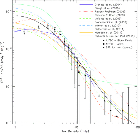
Comparison of the observed, Euclidean-normalized differential source counts from AzTEC surveys and predictions from galaxy evolution models. The differential counts derived from the combined six AzTEC blank fields are shown as the circles (same as Fig. 1), where the black error bars show the 68.3 per cent confidence interval, including systematic uncertainties from cosmic variance (Section 3.3) and flux calibration (Section 3.4). The one-sided extended error bars shown in grey encompass the 68.3 per cent confidence intervals including corrections to the measured counts due to bias from confusion effects, as discussed in Section 5. The squares show the bright source counts derived from ACES fields, as described in Section 4. The triangles show the 1.4 mm source counts from the SPT survey (Vieira et al. 2010), excluding nearby IRAS galaxies and sources whose SEDs are dominated by synchrotron emission. The SPT data have been scaled to 1.1 mm assuming a spectral index of α= 2.65. The curves correspond to predictions from various semi-analytical and phenomenological models taken from the literature, as listed in the legend. See the online journal for a colour version of this figure.
4 BRIGHT SOURCE COUNTS FROM ACES AND SPT
Over the flux densities for which these AzTEC blank-field surveys are sensitive, the source counts are well described by a Schechter function (equation 1), declining exponentially with increasing flux density, since highly luminous galaxies are quite rare. Recent surveys at submm and mm wavelengths covering ≳100 deg2 have been achieved from ground- and space-based observatories, including the Atacama Cosmology Telescope (ACT; Marriage et al. 2011), SPT (Vieira et al. 2010) and the Herschel Space Observatory (Eales et al. 2010; Oliver et al. 2010). These surveys are turning out large numbers of extremely bright, rare objects that are not associated with known nearby systems or strong radio sources, having SEDs consistent with high-redshift, dusty star-forming galaxies. It has been shown that a significant number of these extremely bright systems detected by Herschel, with 500  m flux densities S500≳ 100 mJy, are strongly lensed by foreground galaxies or structure (Negrello et al. 2010; Conley et al. 2011), with magnification factors of μ∼ 10. These lensed galaxies are believed to contribute significantly to the source counts at flux densities greater than those probed by our comparatively small AzTEC surveys. Vieira et al. (2010) have estimated the counts at S1400 > 10 mJy for 1.4-mm sources detected by SPT, excluding those that are associated with nearby galaxies discovered by the Infrared Astronomical Satellite (IRAS) and those with synchrotron-dominated (as opposed to dust-dominated) SEDs. These are shown alongside the AzTEC blank-field counts in Fig. 3, where we have scaled the SPT counts to 1.1 mm assuming a spectral index of α= 2.65, which corresponds to the average spectral index between the observed flux densities at 1.1 and 1.4 mm for a starburst galaxy at z= 3 (Yun & Carilli 2002). The SPT counts, which are believed to be dominated by strongly lensed galaxies, diverge from the exponential fall-off that would be extrapolated from the AzTEC blank-field counts.
During the 2007–2008 observing seasons on ASTE, we observed 37 individual, relatively small (∼300 arcmin2) fields centred on known overdense regions as part of the AzTEC Cluster Environment Survey (ACES). This survey was designed to study the SMG population towards biased fields and includes regions surrounding clusters and protocluster candidates from z= 0.05 to 6, covering a total area of 3.1 deg2. A full description of ACES and first results will be discussed in Zeballos et al. (in preparation).
The ACES fields were not included in our source counts estimate since we specifically wanted to avoid known biased regions. Still, each of the ACES maps includes a relatively large area, far from the central overdense region that is not expected to be influenced by the cluster environment. We see several bright (≥8 mJy) SMGs located far from the biased regions of these ACES maps; from these, we estimate the bright counts at 1.1 mm, which are poorly constrained by our combined blank-field surveys. Since our goal is to fill in the information on the unbiased source counts in the flux range that is not well sampled by the AzTEC blank-field counts or the SPT counts, we apply masks and various selection criteria to the ACES data. We first exclude any SMG detected within 2 arcmin of the centre of the cluster or protocluster core. At z > 0.3 (the minimum redshift of the ACES clusters where S1100≥ 8 mJy sources are found), 2 arcmin corresponds to ≥0.5 Mpc, which is larger than the expected core radii for massive clusters with total masses 1014–1015.7 M⊙ (e.g. Navarro, Frenk & White 1995; Lloyd-Davies, Ponman & Cannon 2000; Kay, Liddle & Thomas 2001). This mask will therefore exclude the major sources of potential biases to the counts, including those from strong lensing and the Sunyaev–Zel’dovich effect, as well as most cluster members. Next, we follow a similar analysis to that followed in Vieira et al. (2010) to exclude nearby galaxies and synchrotron-dominated sources from this sample. We exclude sources which have 2MASS K-band and/or IRAS counterparts located within the AzTEC beam to eliminate low-redshift galaxies. We then check for sources associated with bright radio objects using the Australia Telescope Compact Array 20-GHz survey (Murphy et al. 2010), the Sydney University Molonglo Sky Survey at 843 MHz (Bock, Large & Sadler 1999), and a unified catalogue of radio sources, which combines information from FIRST, NVSS, WENSS, GB6 and SDSS (Kimball & Ivezić 2008). None of the ≥8 mJy ACES sources has radio associations, implying that their SEDs are likely dominated by dust emission. After culling our sample using the above selection criteria, we have a total of 35 S1100≥ 8 mJy sources from these ACES fields.
The ACES bright source counts are shown in Fig. 3 and are listed in Table 2. Given small sample statistics, the errors on the bright source counts derived from the ACES fields are large; however, we see tentative evidence for a divergence of the counts from an exponential fall-off at S1100≳ 13 mJy, and a smooth connection between the AzTEC blank-field counts at S1100 < 12 mJy and the SPT counts at S1100≳ 20 mJy. This upturn may be highlighting the regime at which the source counts become dominated by gravitational lensing effects. On the other hand, it is possible that the 2-arcmin mask is not large enough to remove all cluster members, and the upturn in the counts at S1100≳ 13 mJy is merely reflecting an overdensity of SMGs in the outer regions of the clusters. The source counts at S1100= 1–10 mJy derived from the ACES fields, however, do not support this; Zeballos et al. (2012) find that the ACES source counts are completely consistent with our results from blank fields over these flux densities when the inner regions (1.5 arcmin radii) are masked. Since a real overdensity would be flux-independent, the lack of an excess in the ACES counts at S1100 < 10 mJy suggests that the upturn at S1100≳ 13 mJy is not due to cluster-member contamination.
5 COMPARISON WITH GALAXY EVOLUTION MODELS
With these combined AzTEC surveys, we have put the strongest constraints to date on the blank-field 1.1 mm source counts from S1100= 1 to 12 mJy. These counts provide important information for modelling the formation and evolution of galaxies. A detailed analysis of how these results fit into our current understanding of galaxy evolution is beyond the scope of this paper. However, we can compare our observed 1.1-mm counts to existing predictions from evolutionary models from the literature, many of which have used constraints from 1.1 mm source counts in the past from smaller and/or shallower surveys, in order to motivate modifications to existing models in light of these new constraints. We provide only a qualitative comparison here, since common statistical tests (e.g. the Pearson χ2 test or the Kolmogorov–Smirnov test) do not apply, given the strong correlations between these binned data.
10 such models are shown in Fig. 3. These include predictions from the semi-analytical models of Granato et al. (2004), Baugh et al. (2005) and Wilman et al. (2010), and from the phenomenological models of Rowan-Robinson (2009), Pearson & Khan (2009), Valiante et al. (2009), Franceschini et al. (2010), Béthermin et al. (2011), Marsden et al. (2011) and Rahmati & van der Werf (2011). All of these models assume the standard ΛCDM cosmology, but with slightly different parameters ranging from Λ= 0.7 to 0.734, Ωm= 0.266 to 0.3, and H0= 70 to 75 km s−1 Mpc−1; we have not scaled the model predictions to a uniform cosmology since the differences should be minor. The models show a great deal of dispersion among themselves, differing by as much as a factor of 4 at any given flux density. With the exception of Baugh et al. (2005) and Béthermin et al. (2011), all of the models appear to be largely consistent (within ∼3σ) with the observed source counts at S1100≳ 4 mJy, but many are significantly discrepant at lower flux densities.
With the exception of Béthermin et al. (2011), these models did not include the effects of strong lensing on the counts (which is expected to become important around S1100≳ 15 mJy), and did not use the bright counts measured by SPT as constraints. The general agreement between these models and the ACES and SPT counts is therefore somewhat fortuitous. However, this should not be overinterpreted, since the errors on the ACES and SPT counts are quite large, and the scaling used to convert the 1.4-mm counts from the SPT survey to 1.1 mm is uncertain. We thus limit our discussion in this section to the comparison of these models to the AzTEC blank-field counts.
Considering first the semi-analytical models, the model that best fits the observed 1.1 mm source counts at all flux densities is that of Granato et al. (2004), which considers the evolution of gas within dark matter haloes as driven by gravity, radiative cooling, and feedback from SNe and AGNs. Alternatively, Baugh et al. (2005) modelled the 850- m counts available at the time within the context of hierarchical assembly, where bursts of star formation are triggered solely by galaxy mergers; their model requires a top-heavy IMF in order to explain the number density of SMGs. Although this model overpredicts the 1.1-mm counts by >3σ at S1100 < 5 mJy, minor changes to the model could bring it more in line with our measurements (e.g. changing the dust emissivity).
The semi-analytical model of Wilman et al. (2010) is an extension of their previous work to simulate the extragalactic radio continuum sky, including AGNs and star-forming galaxies, within the framework of their large-scale clustering. Unlike Granato et al. (2004) and Baugh et al. (2005), who use self-consistent radiative transfer calculations to describe the absorption and re-emission of starlight by dust, Wilman et al. (2010) use families of SED templates and FIR–radio relationships for star-forming and AGN-host galaxies to predict the IR-to-submm emission from their simulated radio galaxies, similar to what is done in phenomenological modelling. Their best-fitting model accurately predicts the Spitzer 24–160  m counts, as well as the 850-
 m counts from SCUBA. However, we find that the model of Wilman et al. (2010) overpredicts the 1.1-mm counts by >3σ at S1100≲ 3 mJy. All three of the semi-analytical models considered here predate the large Herschel surveys, and it would be interesting to see how they fare when compared to the counts at shorter submm wavelengths.
We now compare the observed counts to predictions from phenomenological models. The only two that match the blank-field counts within 3σ at all flux densities are those of Rowan-Robinson (2009, with a redshift beyond which evolution is zero of zf= 4) and Pearson & Khan (2009). Both of these models consider only four populations of galaxies, each represented by a single SED, and are therefore some of the simplest models presented here. However, they both used the published 1.1 mm source counts from the AzTEC/GOODS-N field (Perera et al. 2008) to constrain their models, so the agreement with the combined-field source counts is not surprising.
Like those of Rowan-Robinson (2009) and Pearson & Khan (2009), the phenomenological models of Valiante et al. (2009), Franceschini et al. (2010) and Marsden et al. (2011) used constraints from source counts ranging from 24 to  m, but did not use constraints on the 250–500
  m counts from Herschel surveys – though Franceschini et al. (2010) and Marsden et al. (2011) do consider counts at these wavelengths from BLAST data. It is interesting to note that all five of these models overpredict the Herschel
 m source counts (Clements et al. 2010; Glenn et al. 2010; Oliver et al. 2010). We find that the Valiante et al. (2009) and Franceschini et al. (2010) models provide a decent fit (within 3σ) to the 1.1 mm source counts in all but the two lowest flux bins. Valiante et al. (2009) did not use the source counts at 1.1 mm to constrain their models, which at the time of their publication were limited to data from relatively small and/or shallow fields (Laurent et al. 2005; Bertoldi et al. 2007; Perera et al. 2008). In comparison, Franceschini et al. (2010) did use constraints on the 1.1-mm counts from the AzTEC/JCMT survey of COSMOS (Austermann et al. 2009), and their model is in somewhat better agreement with our combined-field counts. However, compared to the other AzTEC fields shown in Fig. 1, the AzTEC/JCMT survey targeted a smaller and considerably overdense region within COSMOS, so it is not too surprising that the model from Franceschini et al. (2010) now overpredicts the counts at low flux densities. Marsden et al. (2011) used the counts determined from the AzTEC/SHADES fields to fit their model, but it predates the correction to the AzTEC transfer function (Downes et al. 2011); it now therefore underpredicts the combined-field counts at flux densities 3 < S1100 < 5 mJy, and overpredicts the counts in the lowest flux bin, by >3σ. However, this model is in better agreement with the counts at S1100 < 3 mJy than those of Valiante et al. (2009) and Franceschini et al. (2010).
We consider two phenomenological models that include recent constraints on the 250–500  m counts from Herschel. The Béthermin et al. (2011) model underpredicts the 1.1 mm source counts by >3σ at flux densities 2 < S1100 < 6 mJy. Those authors used the 1.1 mm counts from the AzTEC surveys of GOODS-S (Scott et al. 2010) and SHADES (Austermann et al. 2010) to constrain their model; however, the published counts from those surveys were systematically low due to the error in our transfer function estimate. On the other hand, Rahmati & van der Werf (2011) did not use the 1.1 mm counts from published AzTEC surveys to constrain their model; however, they did compare their best-fitting model to these data and showed that they are largely consistent, though their model overpredicts the 1.1 mm counts at S1100≲ 3 mJy.
As demonstrated in Section 3.2, we expect the extracted 1.1 mm counts to be moderately biased due to confusion effects. Given the small statistical errors on the measured counts from these surveys, these biases should be taken into account when assessing the agreement between these data and various models. In Fig. 3, we include one-sided extended error bars (in grey) to account for the bias in our measurements due to confusion effects. These error bars encompass the 68.3 per cent confidence interval on the corrected counts, where we have used the results from the simulations in Section 3.2 to estimate correction factors to the measured counts. While this is only an approximate correction for the effects of confusion, it is sufficient for our purpose of qualitatively comparing our measurements to predictions from galaxy evolution models. As shown in Fig. 3, extending the uncertainty on the counts naturally brings the data and models into somewhat better agreement; however, the discrepancies at S1100≳ 4 mJy remain large, and the main conclusions from the comparisons to various evolution models above are unchanged.
6 DISCUSSION
Given that galaxy evolution models using semi-analytical methods provide some insight into the physical processes occurring within galaxies (albeit with several simplistic assumptions), it is interesting to compare these predictions with our measured counts. The best-fitting semi-analytical model to the combined 1.1-mm counts is that of Granato et al. (2004). That model was able to reproduce the 850  m source counts and their redshift distribution measured at that time, as well as the K-band luminosity function of massive spheroids at z= 1.5. A key feature of their model is that feedback from SNe is more effective in slowing down the rate of star formation in shallower potential wells, so that star formation progresses more rapidly within the most massive haloes. This scenario seems to be consistent with recent evidence in favour of ‘downsizing’ of SMGs (e.g Dye et al. 2008), where, contrary to the hierarchical collapse of dark matter, star formation in the early Universe predominately takes place within the most massive systems and progresses to lower mass systems at later times (e.g. Cowie et al. 1996; Bundy et al. 2006; Franceschini et al. 2006; Mobasher et al. 2009; Magliocchetti et al. 2011). This idea is supported by the strong evolution of the luminosity function determined from phenomenological models, which implies that the most luminous star-forming galaxies (with IR luminosities LIR≳ 1011 L⊙) dominate at z≳ 1.5, while normal galaxies dominate at lower redshifts.
It is interesting to note that, of the phenomenological models discussed here, only that of Franceschini et al. (2010) is consistent with the turnover in the Euclidean-normalized counts at S1100≲ 2 mJy; however, like all of these models, it significantly over-predicts the counts at these faint flux densities, which have until now been only poorly constrained. This observed turnover in our data is statistically significant. If we fit our measured counts near the apparent peak at S1100= 2.4 and 3.4 mJy assuming no evolution (i.e. flat in Euclidean-normalized space), we find that the observed counts at S1100= 1.4 mJy fall short of this no-evolution model by 5σ. The discrepancies between the predictions from these phenomenological models and the observed counts at faint flux densities may be highlighting our limited knowledge of both the SEDs and the density of low-luminosity (LFIR < 1010 L⊙) galaxies in the local Universe and, in turn, the faint end of the local luminosity function (see Chapin, Hughes & Aretxaga 2009a, and references therein). In their phenomenological modelling of the 70–1100  m detected populations, Marsden et al. (2011) find that the model which best fits the observed counts and redshift distributions overpredicts the CIRB at these wavelengths. They explore whether simple modifications to the SEDs of low-luminosity galaxies – to which the source counts are not sensitive, but which dominate the CIRB – can improve the fit to the CIRB. They find that by assigning the warmest SEDs to LFIR < 109 L⊙ galaxies, they can bring the CIRB prediction into agreement with the observed value. It is therefore possible that poor knowledge of the SEDs of local faint galaxies also limits how well phenomenological models can predict the faint end of the 1.1 mm source counts. Alternatively, evolutionary models that consider two distinct populations evolving separately – where low-luminosity galaxies evolve less strongly and thus reduce the number of cold galaxies at high redshift (e.g. Valiante et al. 2009) – can also successfully match both the observed source counts and the CIRB. If this is the case, the turnover at the faint end of the AzTEC 1.1 mm counts may be providing important new information on the evolution of low-luminosity systems.
At the other extreme, accounting for the observed number density of bright SMGs poses a significant challenge for existing theoretical models (e.g. Hayward et al. 2011). As discussed in Section 4, there is evidence for a bias in the observed source counts at S1100≳ 15 mJy arising from background SMGs that are strongly lensed by foreground structure (Vieira et al. 2010). Although lensing is not expected to significantly bias the observed 1.1 mm counts at lower flux densities, current modelling of this effect is necessarily simplistic and not well informed by observations (Negrello et al. 2007; Paciga, Scott & Chapin 2009; Lima, Jain & Devlin 2010; Béthermin et al. 2011). Austermann et al. (2010) and Aretxaga et al. (2011) have shown that S1100≳ 5 mJy sources are spatially correlated with z≲ 1.1 optical/IR galaxies in COSMOS, suggesting that galaxy–galaxy and galaxy–group lensing at moderate amplification levels may bias the observed counts high, even at more modest flux densities. Wang et al. (2011a) find a spatial correlation between foreground optical/IR galaxies from SDSS and Spitzer/IRAC with high-redshift SMGs detected by Herschel in the Lockman-SWIRE field; since the redshift distributions of these different populations do not overlap significantly, this is strong evidence that the correlation arises from gravitational lensing. We have repeated the analysis of Wang et al. (2011a) for the individual AzTEC fields for which SDSS and/or IRAC data are available, and find that only the COSMOS field shows a tentative (∼2σ) correlation with the low-redshift galaxy samples – consistent with the findings in Aretxaga et al. (2011). Since we are sampling much smaller fields than Herschel Lockman-SWIRE, our statistical power is limited. Still, these results hint that lensing may have a significant effect on the observed source counts, even at moderate flux densities.
The observed counts can also be significantly biased if a large fraction of the SMGs detected as single point sources in low-resolution surveys, such as those carried out with AzTEC, LABOCA and Herschel, are actually multiple systems blended by the large beam. High-resolution (∼2 arcsec) interferometric imaging with the Submillimeter Array of an unbiased, flux-limited (S1100 > 5.5 mJy) sample of 15 AzTEC-detected SMGs discovered in COSMOS showed that only two (13 per cent) are resolved into two, physically unassociated galaxies (Younger et al. 2007, 2009). On the other hand, simulations designed to match the observed source counts suggest that the fraction of multiple, blended galaxies for SMGs detected in low-resolution observations can be even higher. Wang et al. (2011b) predict that ∼1/3 of the S850 > 5 mJy SCUBA sources are actually multiple galaxies blended by the beam. Similarly, using the same kind of simulations as described in Section 3.2, Scott et al. (2010) demonstrated that ∼25 per cent of SMGs detected as single point sources in the confusion-limited AzTEC map of GOODS-S are likely to be two or more sources blended together. However, our simulations in Section 3.2 suggest that this has only a small effect on the measured source counts.
There are nevertheless potential biases to the observed source counts that we have not studied in our simulations: in particular, the effects of galaxy clustering. There are currently only weak constraints on the clustering strength of bright SMGs (e.g. Blain et al. 2004; Weiß et al. 2009; Lindner et al. 2011; Williams et al. 2011), and the clustering strength of faint mm-selected sources below the confusion limit has not been measured. If these faint, but much more numerous galaxies are strongly clustered, the biases to the measured 1.1 mm source counts could be much larger than those predicted by our simulations in Section 3.2. Our lack of knowledge on the clustering properties of sub-mJy SMGs precludes a more rigorous study of the potential biases to the measured source counts from galaxy clustering. The fraction of blended SMGs detected in low-resolution surveys, and whether this leads to significant biases to the source counts, can be addressed in future observations with ALMA.
7 SUMMARY AND CONCLUSIONS
We have combined previously published data from six blank-field surveys at 1.1 mm taken with AzTEC, totalling 1.6 deg2 in area with rms depths of 0.4–1.7 mJy beam−1, in order to derive the strongest constraints to date on the 1.1 mm extragalactic source counts from S1100= 1 to 12 mJy. We use the well-tested bootstrap sampling method on the source catalogues to derive the counts, which allows for an accurate estimate of statistical errors, including correlations among the selected flux bins. Given the large total area sampled, we expect a systematic uncertainty in the counts arising from cosmic variance of only 3.9 per cent. As discussed in Sections 3.3 and 3.4, it is important to include systematic uncertainties from cosmic variance and flux calibration (∼5 per cent) into the total error on the observed source counts, since these must be considered when using the counts to constrain parameters in galaxy evolution modelling (e.g. as done in Béthermin et al. 2011). We have included these systematic uncertainties in the total errors reported on our combined-field source counts by incorporating them directly into the bootstrap sampling method, and we list these in Tables 2–4.
Comparing the observed 1.1 mm source counts to predictions from several galaxy evolution models, we find that the agreement at flux densities S1100≳ 4 mJy is generally good. Given that most of these models had been fitted to bright source counts at 850  m and/or 1.1 mm from previously published surveys, this agreement is expected. However, we find significant (≳3σ) discrepancies between the combined-field 1.1 mm counts and many of these models at S1100≲ 4 mJy. Similarly, with the exception of the most recent phenomenological models that include constraints from Herschel surveys, many of the models overpredict the counts at 250–500
  m. The data presented here provide strong constraints – highly complementary to those from Herschel surveys at shorter wavelengths – that should be used in future modelling of the formation and evolution of IR-bright galaxies.
Of the semi-analytical models considered in this paper, the model of Granato et al. (2004) provides the best match to the 1.1 mm source counts. This model is consistent with downsizing, in which the bulk of star formation activity progresses from more massive to less massive galaxies over time – a scenario that is also supported by most phenomenological models that can describe the counts and redshift distribution of IR-bright sources. However, for the model of Baugh et al. (2005), where the build-up of stellar systems is consistent with hierarchical formation, only minor modifications are required to improve its agreement with the observed source counts at 1.1 mm. A better understanding of the physical processes of gas cooling and feedback is needed in order to provide information on which scenario best describes the assembly of massive galaxies.
For the first time, we have been able to strongly constrain the 1.1 mm counts at S1100 < 3 mJy, and we measure a turnover in the Euclidean-normalized counts at S1100≲ 2 mJy which none of the evolutionary models considered here is able to reproduce. This either reflects our limited knowledge of the SEDs of low-luminosity galaxies in the local Universe, or motivates modifications to the evolution of faint galaxies at high redshift. Wide-area surveys at 60–500  m with Herschel (e.g. H-ATLAS, Eales et al. 2010) and future surveys at 450
  m with SCUBA-2 and at 1.1 mm with AzTEC on the Large Millimeter Telescope (LMT) will provide measurements of the SEDs of a large, unbiased sample of faint nearby galaxies, which, in turn, will allow for improved modelling of the evolution of these systems at high redshift.
While there is already considerable evidence that the counts at S1100≳ 15 mJy are biased high by strong-lensing effects, some groups have also demonstrated that galaxy–galaxy and galaxy–group lensing with moderate amplification may affect the observed counts at more modest flux densities (S1100∼ 5 mJy). Furthermore, galaxies detected as single point sources in low-resolution surveys, such as those taken with AzTEC, can also bias our measurements of the source counts if a significant fraction of these ‘sources’ are really two or more galaxies blended by the large beam. The effects of lensing and blending on the measured source counts are poorly understood, and may lead to inaccurate predictions from galaxy evolution models. High-resolution imaging of statistically significant samples of SMGs with ALMA will be possible in the near future, and this will greatly aid in quantifying the degree to which lensing and blended galaxies bias the observed source counts.
Compared to observations at shorter submm wavelengths from Herschel, surveys at 1.1 mm sample (on average) galaxies at higher redshifts, as the negative k-correction for observations at longer wavelengths extends to z∼ 10. Indeed, a growing number of 1.1 mm bright SMGs are found to be at z > 4 (Coppin et al. 2009; Daddi et al. 2009a,b; Riechers et al. 2010; Capak et al. 2011; Smolčić et al. 2011). The source counts at 1.1 mm presented here, and those derived from future surveys with AzTEC on LMT, will therefore provide crucial information on the evolution of star-forming galaxies within the first ∼2 Gyr after the big bang, where observations at shorter submm wavelengths provide few constraints.
We thank Chris Pearson and Alberto Franceschini for providing us with predictions of the 1.1 mm source counts from their galaxy evolution models. KSS is supported by the National Radio Astronomy Observatory, which is a facility of the National Science Foundation operated under cooperative agreement by Associated Universities, Inc. IA and DHH acknowledge support from CONACyT projects #39953-F. BH is supported by a Research Fellowship for Young Scientists from the Japan Society of the Promotion of Science. JSD acknowledges the support of the Royal Society via a Wolfson Research Merit award, and also the support of the European Research Council via the award of an Advanced Grant. This work is supported in part by grants #0907952 and #0838222 from the National Science Foundation. This work is supported in part by the MEXT Grant-in-Aid for Specially Promoted Research (#20001003) and Scientific Research on Priority Areas (#15071202). The ASTE project is driven by the Nobeyama Radio Observatory, a branch of the NAOJ, in collaboration with the University of Chile and Japanese institutes including the University of Tokyo, Nagoya University, Osaka Prefecture University, Ibaraki University and Hokkaido University. The James Clerk Maxwell Telescope is operated by the Joint Astronomy Centre on behalf of the Science and Technology Facilities Council of the United Kingdom, the Netherlands Organization for Scientific Research, and the National Research Council of Canada.
Footnotes
REFERENCES
