


Abstract
We present a detailed auto-consistent study of the nearest blue compact dwarf galaxy NGC 6789 by means of optical and ultraviolet (UV) archive photometry data and optical long-slit Intermediate dispersion Spectrograph and Imaging System-William Herschel Telescope (WHT) spectroscopy observations of the five brightest star-forming knots. The analysis of the spectra in all knots allowed the derivation of ionic chemical abundances of oxygen, nitrogen, sulphur, argon and neon using measures of both the high- and low-excitation electron temperatures, leading to the conclusion that NGC 6789 is chemically homogeneous with low values of the abundance of oxygen in the range 12+log(O/H) = 7.80–7.93, but presenting at the same time higher values of the nitrogen-to-oxygen ratio than expected for its metal regime.
We used archival Hubble Space Telescope/Wide-Field Planetary Camera 2 (HST/WFPC2) F555W and F814W observations of NGC 6789 to perform a photometric study of the colour–magnitude diagram (CMD) of the resolved stellar populations and derive its star formation history (SFH), which is compatible with the presence of different young and old stellar populations whose metallicities do not necessarily increase with age. We fit the observed optical spectrum in all the five knots using the starlight code and a combination of single stellar populations following the SFH obtained from the CMD. We compare the resulting stellar masses and the relative fractions of the ionizing populations with a non-constrained SFH case. The properties of the younger populations were obtained using cloudy photoionization models, giving similar ages in all the knots in the range 3–6 Myr and the estimation of the dust absorption factor, which correlates with the observed GALEX far-ultraviolet–near-ultraviolet colour indices. The total photometric extinction and dust-absorption corrected Hα fluxes were finally used to derive the star formation rates.
1 INTRODUCTION
Blue compact dwarf galaxies (BCDs) are known by their intense processes of star formation. These make that their optical spectra were dominated by the blue light from massive young stars and the bright emission lines from the ionized gas, so they are also called H ii galaxies.
Their high specific star formation rates (SFRs) and their low gas-phase metallicities were taken as evidence that these galaxies were undergoing their first bursts of star formation (Sargent & Searle 1970). In fact, one of the most important aspects about BCDs is that they constitute an important link to the high-redshift Universe and the early epoch of galaxy formation (Bergvall & Östlin 2002). During the last decade, however, deep imaging of BCDs showed that in addition to bright young stars from the present starburst, most of them have an underlying older stellar population (Papaderos et al. 1996; Aloisi, Tosi & Greggio 1999; Östlin 2000).
One of the challenges of the BCDs is to reconcile their low observed metallicity with the relatively high SFR in these galaxies. Matteucci & Chiosi (1983) proposed three possible mechanisms to explain this fact: (1) variations in the initial mass function (IMF), (2) accretion of metal-poor gas and (3) galactic winds powered by supernovae explosions. According to numerical models, it seems that the last mechanism is the most simple to reproduce the observed properties (see Tolstoy, Hill & Tosi 2009 and references therein for a detailed explanation).
The star formation history (SFH) and the metal content of BCDs must be figured out in order to shed some light on these questions. In the case of SFH, although some advances have been done by means of the fitting of the optical spectrum with stellar populations synthesis (Pérez-Montero et al. 2010), one of the most reliable methods consists of the analysis of colour–magnitude diagrams (CMDs). However, this is limited to the closest objects whose stellar population can be resolved. Another important contribution comes from the study of the ionic chemical abundances of elements with a different nucleosynthetic origin, such as oxygen and nitrogen (Mollá et al. 2006). These chemical abundances can be derived very accurately in the metal-poor gas phase of BCDs, where the cooling rate is not efficient, increasing the electron temperature of the ionized gas and enhancing the emissivity of the collisional lines necessary to derive the ionic abundances following the method based on the determination of the electron temperature (Pérez-Montero & Díaz 2003; Hägele et al. 2006).
NGC 6789 is, according to Drozdovsky et al. (2001), the closest BCD to our Galaxy, with a distance modulus of (m−M) = 27.80 or a distance of 3.6 Mpc. This value yields a linear scale of 17.5 pc arcsec−1. Drozdovsky & Tikhonov (2000) imaged NGC 6789 from the ground. They found that it belongs to the iE1 subtype (following the Loose & Thuan 1986 classification), exhibiting the morphology most characteristic of the vast majority of BCDs. NGC 6789 presents several Hα emission knots which show the evidence of actual star formation activity. It also shows a high surface brightness in its central region and a small radial velocity (V0=−141 km s−1; Karachentsev & Makarov 1998). NGC 6789’s closeness, spatial isolation and morphology offer the prospect of studying the structure, SFH and metallicity of different star-forming knots within the same BCD.
To investigate these issues, we obtained simultaneous blue and red long-slit observations with the Intermediate dispersion Spectrograph and Imaging System (ISIS) double-arm spectrograph at the 4.2-m William Herschel Telescope (WHT), of the brightest five knots of NGC 6789. We also used archival data from the Hubble Space Telescope/Wide-Field Planetary Camera 2(HST/WFPC2), the Galaxy Evolution Explorer (GALEX) and the Hα narrow filter, and B and R broad filters. These images were used to derive the SFH and to give an observational input to derive the properties of the ionizing populations with the aid of photoionization models. These were also used to provide more accurate chemical abundances in each one of the five studied knots of this galaxy and to better understand their differential chemical evolution.
In the following section, the long-slit WHT observations and reduction are described and the results from the analysis are presented. In Section 3, the optical and ultraviolet (UV) photometry are described together with the resolved stellar photometry. Finally, we discuss all these results in Section 4 and conclusions are presented in Section 5.
2 LONG-SLIT SPECTROSCOPY
2.1 Observations and reduction
The long-slit spectrophotometric observations of NGC 6789 were obtained using the ISIS double-beam spectrograph mounted on the 4.2-m WHT of the Isaac Newton group (ING) at the Roque de los Muchachos Observatory on the Spanish island of La Palma. They were acquired on 2005 July 8 during one single night observing run and under photometric conditions, with an average seeing of 0.7 arcsec. The EEV12 and Marconi2 detectors were attached to the blue and red arms of the spectrograph, respectively. The R600B grating was used in the blue, covering the wavelength range 3670–5070 Å (centred at λc= 4370 Å), giving a spectral dispersion of 0.45 Å pixel−1. On the red arm, the R316R grating was mounted in two different central wavelengths providing a spectral range from 5500 to 7800 Å (λc= 6650 Å) and from 7600 to 9900 Å (λc= 8750 Å) with a spectral dispersion of 0.86 Å pixel−1. To reduce the readout noise of our images, the observations were taken with the ‘slow’ CCD speed. The pixel size for this set-up is 0.2 arcsec for both spectral ranges. The slit width was 1 arcsec, which, combined with the spectral dispersions, yields spectral resolutions of about 1.0 and 3.5 Å full width at half-maximum (FWHM) in the blue and red arms, respectively. The instrumental configuration and other details on the exposures are given in the journal of observations in Table 1.
WHT instrumental configuration.
| Slit position | Spectral range (Å) | Disp. (Å pixel−1) | FWHM (Å) | Spatial res. (arcsec pixel−1) | Exposure time (s) |
| S1 | 3670–5070 | 0.45 | 1.0 | 0.2 | 4 × 900 |
| S1 | 5500–7800 | 0.86 | 3.5 | 0.2 | 2 × 900, 1 × 300 |
| S1 | 7600–9900 | 0.86 | 3.5 | 0.2 | 2 × 900 |
| S2 | 3670–5070 | 0.45 | 1.0 | 0.2 | 5 × 900 |
| S2 | 5500–7800 | 0.86 | 3.5 | 0.2 | 2 × 900, 1 × 300 |
| S2 | 7600–9900 | 0.86 | 3.5 | 0.2 | 2 × 900 |
Several bias and sky flat-field frames were taken at the beginning and at the end of the night in both arms. In addition, two lamp flat-fields and one calibration lamp exposure were taken for each telescope position. The calibration lamp used was +CuAr.
The images were processed and analysed with iraf2 routines in the usual manner. The procedure included cosmic rays removal, bias subtraction, division by a normalized flat-field and wavelength calibration. Typical wavelength fits to second- to third-order polynomials were performed using around 40 lines in the blue and 20–25 lines in the red. These fits were done at 100 different locations along the slit in both arms (beam size of 10 pixels) obtaining rms residuals between ∼0.1 and ∼0.2 pixels. In the last step, the spectra were corrected for atmospheric extinction and flux calibrated. For both arms, BD+254655 standard star observations were used, allowing a good spectrophotometric calibration with an estimated accuracy of about 5 per cent.
Unfortunately, the sky subtraction in the spectral range from 7600 to 9900 Å left strong residuals from night-sky emission lines and telluric absorption, leaving this part of the spectra unusable and, therefore, we were not able to measure with enough accuracy the [S iii] λλ 9069, 9532 Å lines in any of the five knots.
Fig. 1 shows the Hα image and continuum contours in the R band from Gil de Paz et al. (2003) in order to illustrate the position of the slits in relation to the position of the bursts of star formation and the host galaxy. We also show elliptical regions in Hα taken to measure the total Hα and GALEX flux of the knots (see Section 3.1). The five knots are labelled with the first alphabet letters. Knots A and C were taken at a position angle (PA) of 138°, which in average is close to the parallactic angle. In the case of knots B, D and E, the slit was at PA = 76°, which is in average ≈40° off the parallactic angle. Therefore, the observations in this second position can be affected by a certain differential atmospheric refraction. Nevertheless, taking into account the curves given by Filippenko (1982) for the mean air mass during the observations (≈1.30), we calculated that the angular deviation between [Oii] and [Sii] is not larger than the slit width at this PA. Besides, we checked that the emission-line ratios in the spatial position where both slit positions intersect do not vary in more than the quoted errors. Nevertheless, the line measurement errors of the second slit position (B, D and E knots) might be larger due to this effect. For the sake of comparison, we also plot in Fig. 1 part of the rectangle encompassing the field of view (FOV) of the PC chip of the WFPC2 data used to obtain the resolved stellar photometry (see Section 3.2).
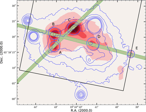
Hα image of NGC 6789 from Gil de Paz, Madore & Pevunova (2003) with the identification of the observed knots (labelled from A to E). We show the regions for which the Hα flux was measured and the position of the two slits for the observations described in the text. The R-band contours show the position of the host galaxy. Finally, we also plot part of the rectangle encompassing the FOV of the PC chip of the WFPC2 data used to obtain the resolved stellar photometry described in Section 3.2. North is up and east is towards the left-hand side.
2.2 Line intensities and reddening correction
The optical calibrated spectra of the five observed knots with some relevant identified emission lines are shown in Fig. 2. The spectrum of each knot is split into two panels.
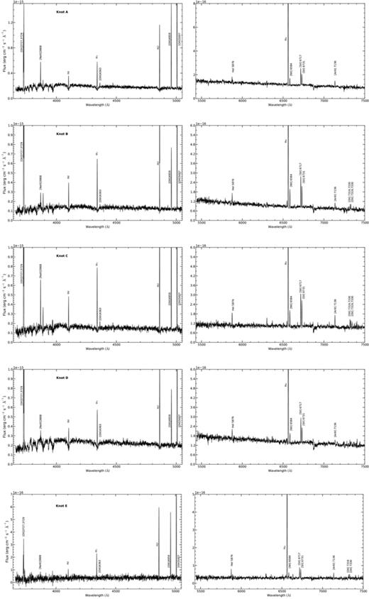
Blue and red spectra for the knots A–E of NGC 6789.
Underlying stellar population in star-forming galaxies has several effects in the measure of the emission lines produced by the ionized gas. Balmer and Paschen emission lines are depressed by the presence of absorption wings of stellar origin and does not allow the measure of their fluxes with acceptable accuracy (Díaz 1988). All the properties derived from ratios that involve these lines, like reddening or ionic abundances, will be affected.
We subtracted from the observed spectra the spectral energy distribution of the underlying stellar population found by the spectral synthesis code starlight3 (Cid Fernandes et al. 2004, 2005; Mateus et al. 2006). starlight fits an observed continuum spectral energy distribution using a combination of the synthesis spectra of different single stellar populations (SSPs; also known as instantaneous burst) using a χ2 minimization procedure. We chose for our analysis the SSP spectra from Bruzual & Charlot (2003), based on the STELIB library of Le Borgne et al. (2003), Padova 1994 evolutionary tracks and a Chabrier (2003) IMF between 0.1 and 100 M⊙. The metallicity of the libraries was strictly constrained following the results derived from Section 4.1. Thus, we fixed the metallicity of the stellar populations to Z= 0.004 (≈3/10 Z⊙4) for the interval log(age) = [8.1,8.5] and Z= 0.001 (≈1/12 Z⊙) for log(age) = {6.0, 6.4, 6.6, 6.8, 7.0, 7.1, 7.2, 7.9, 8.0, 8.1, 8.2, 8.3, 9.1, 9.2, 9.3, 9.7, 9.8, 9.9, 10.0, 10.1} shown in the SFH solution (see Fig. 5). As explained in Section 4.1, although both metallicities appear in the youngest burst (<12 Myr) SFH solution, we assigned the lower metallicity to this event according to the abundances derived in Section 2.4. The starlight code solves simultaneously the ages and relative contributions of the different SSPs and the average reddening. The reddening law from Cardelli, Clayton & Mathis (1989) with RV= 3.1 was used. Prior to the fitting procedure, the spectra were shifted to the rest frame and re-sampled to a wavelength interval of 1 Å in the entire wavelength range by interpolation, as required by the program. Bad pixels and emission lines were excluded from the final fits.
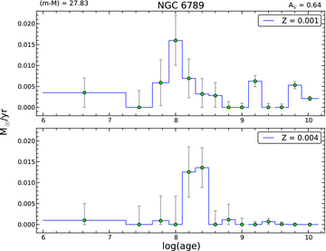
Best starfish SFH fit derived from the HST optical observations of the resolved stellar populations for NGC 6789. The best distance modulus and extinction values are also shown.
It should be noted that while emission lines can be masked out, this is not possible for the nebular continuum emission. We tested the contribution of this emission using starburst99 libraries (Leitherer et al. 1999) in the same starlight models and we checked that the nebular continuum does not affect significantly either the subtraction of the underlying continuum or the determination of the stellar mass, consistent with the weak gas emission in this galaxy.
The H i series (emitted as a consequence of recombination) were used to determine the extinction, comparing the observed line ratios with the expected theoretical values. Case B (optically thick in all the Lyman lines) is the best simple approximation to describe the physical conditions in the ionization of the gas. This method takes advantage of the fact that the ratio between the emissivities of two hydrogen recombination lines, which depends on electron temperature and density, is almost constant. As an example, the ratio between the emissivities of Hα and Hβ is 2.86 for the case B with ne= 100 cm−3 and Te= 10 000 K, and this value varies less than 10 per cent in the range of interest of temperatures and densities for an H ii region. We used an iterative method to estimate them, taking as starting values those derived from the measured [S ii] λλ6717, 6731 Å and [O iii] λλ4363, 4959, 5007 Å. A least-squares fit of the measured decrements to the theoretical ones, computed based on the data by Storey & Hummer (1995), was performed that provides the reddening coefficient, c(Hβ), and adopting the extinction law given by Cardelli et al. (1989) with RV= 3.1. Due to the large error introduced by the presence of the underlying population, only the strongest Balmer emission lines (Hα, Hβ, Hγ and Hδ) were used.

 is the error in the observed line flux,
  represents the standard deviation in a box near the measured emission line and stands for the error in the continuum placement, N is the number of pixels used in the measure of the line flux, EW is the line equivalent width, and Δ is the wavelength dispersion in Å pixel−1 (Gonzalez-Delgado et al. 1994). This expression takes into account the error in the continuum and the photon count statistics of the emission line.
Table 2 gives the equivalent widths and the emission-line fluxes relative to 1000 F(Hβ), before and after reddening correction, in the optical spectra of the five observed knots, together with the reddening constants and their errors, their corresponding A(V) value6 and the extinction-corrected Hβ flux. We also provide the adopted reddening curve, f(λ) normalized to Hβ. The errors in the emission-line ratios were obtained by propagating in quadrature the observational errors in the emission-line fluxes and the reddening constant uncertainties.
Observed and reddening-corrected relative line intensities [F(Hβ) =I(Hβ) = 1000] with their corresponding errors for the five knots. The adopted reddening curve, f(λ) (normalized to Hβ), the equivalent width of the emission lines, the extinction-corrected Hβ intensity, the reddening constant c(Hβ) and the corresponding A(V) are also given.
| λ (Å) | f(λ) | F(λ) | EW (Å) | I(λ) | F(λ) | EW (Å) | I(λ) | ||||
| NGC 6789-A | NGC 6789-B | ||||||||||
| 3726 [O ii] | 0.322 | 896 ± 19 | −15.0 | 979 ± 63 | 1186 ± 17 | −34.9 | 1277 ± 80 | ||||
| 3729 [O ii] | 0.322 | 1241 ± 16 | −20.7 | 1357 ± 84 | 1744 ± 16 | −51.9 | 1878 ± 116 | ||||
| 3835 H9 | 0.299 | 37 ± 10 | −0.6 | 40 ± 11 | 80 ± 4 | −3.5 | 85 ± 7 | ||||
| 3868 [Ne iii] | 0.291 | 302 ± 17 | −2.8 | 327 ± 26 | 153 ± 14 | −3.7 | 164 ± 17 | ||||
| 3889 He i+H8 | 0.286 | 153 ± 6 | −2.6 | 166 ± 12 | 146 ± 10 | −4.5 | 156 ± 14 | ||||
| 3968 [Ne iii]+H7 | 0.266 | 81 ± 8 | −1.3 | 88 ± 10 | − | − | − | ||||
| 4102 Hδ | 0.229 | 247 ± 5 | −3.9 | 263 ± 16 | 248 ± 16 | −6.7 | 261 ± 22 | ||||
| 4340 Hγ | 0.157 | 454 ± 11 | −7.2 | 474 ± 28 | 448 ± 7 | −12.4 | 465 ± 26 | ||||
| 4363 [O iii] | 0.149 | 63 ± 3 | −0.7 | 66 ± 5 | 23 ± 4 | −0.4 | 23 ± 4 | ||||
| 4471 He i | 0.115 | 36 ± 4 | −0.4 | 37 ± 5 | 37 ± 6 | −0.7 | 39 ± 7 | ||||
| 4861 Hβ | 0.000 | 1000 ± 10 | −17.3 | 1000 ± 47 | 1000 ± 12 | −29.1 | 1000 ± 48 | ||||
| 4959 [O iii] | −0.026 | 1240 ± 12 | −16.0 | 1231 ± 57 | 512 ± 12 | −11.4 | 509 ± 26 | ||||
| 5007 [O iii] | −0.038 | 3801 ± 13 | −50.1 | 3762 ± 167 | 1492 ± 9 | −33.0 | 1479 ± 66 | ||||
| 5876 He i | −0.203 | 102 ± 14 | −1.6 | 97 ± 14 | 96 ± 16 | −2.3 | 92 ± 16 | ||||
| 6312 [S iii] | −0.264 | 11 ± 2 | −0.2 | 10 ± 2 | 16 ± 5 | −0.5 | 16 ± 5 | ||||
| 6548 [N ii] | −0.296 | 28 ± 5 | −0.5 | 26 ± 5 | 61 ± 9 | −1.8 | 57 ± 8 | ||||
| 6563 Hα | −0.298 | 3038 ± 29 | −57.0 | 2797 ± 38 | 3003 ± 15 | −89.3 | 2807 ± 20 | ||||
| 6584 [N ii] | −0.300 | 136 ± 10 | −2.5 | 126 ± 9 | 186 ± 11 | −5.6 | 174 ± 10 | ||||
| 6717 [S ii] | −0.318 | 277 ± 10 | −5.0 | 254 ± 10 | 314 ± 9 | −9.5 | 292 ± 8 | ||||
| 6731 [S ii] | −0.320 | 188 ± 10 | −3.4 | 172 ± 9 | 217 ± 10 | −6.6 | 202 ± 9 | ||||
| 7136 [Ar iii] | −0.374 | 112 ± 7 | −2.4 | 101 ± 7 | 76 ± 7 | −2.7 | 70 ± 7 | ||||
| 7319 [O ii] | −0.398 | - | - | - | 46 ± 6 | −1.6 | 42 ± 6 | ||||
| 7330 [O ii] | −0.400 | - | - | - | 35 ± 4 | −1.2 | 32 ± 4 | ||||
| I(Hβ)(erg s−1 cm−2) | 2.70e−15 | 3.19e−15 | |||||||||
| c(Hβ) | 0.12 ± 0.02 | 0.10 ± 0.02 | |||||||||
| A(V) | 0.26 ± 0.04 | 0.21 ± 0.04 | |||||||||
| NGC 6789-C | NGC 6789-D | ||||||||||
| 3726 [O ii] | 0.322 | 940 ± 13 | −29.1 | 1020 ± 64 | 1159 ± 26 | −15.4 | 1267 ± 82 | ||||
| 3729 [O ii] | 0.322 | 1377 ± 12 | −42.4 | 1494 ± 92 | 1712 ± 21 | −22.5 | 1871 ± 116 | ||||
| 3835 H9 | 0.299 | 47 ± 9 | −1.4 | 50 ± 10 | - | - | - | ||||
| 3868 [Ne iii] | 0.291 | 300 ± 12 | −5.2 | 323 ± 23 | 105 ± 9 | −0.9 | 114 ± 12 | ||||
| 3889 He i+H8 | 0.286 | 169 ± 12 | −5.5 | 182 ± 17 | 167 ± 20 | −2.4 | 180 ± 24 | ||||
| 3968 [Ne iii]+H7 | 0.266 | 74 ± 9 | −2.3 | 79 ± 11 | - | - | - | ||||
| 4102 Hδ | 0.229 | 246 ± 16 | −5.9 | 261 ± 22 | 244 ± 7 | −3.2 | 260 ± 16 | ||||
| 4340 Hγ | 0.157 | 446 ± 7 | −12.4 | 464 ± 26 | 444 ± 10 | −5.3 | 464 ± 27 | ||||
| 4363 [O iii] | 0.149 | 59 ± 3 | −1.3 | 61 ± 5 | 24 ± 8 | −0.2 | 25 ± 8 | ||||
| 4471 He i | 0.115 | 37 ± 5 | −0.7 | 38 ± 6 | 36 ± 6 | −0.3 | 37 ± 7 | ||||
| 4686 He ii | 0.050 | 26 ± 5 | −0.5 | 26 ± 5 | - | - | - | ||||
| 4861 Hβ | 0.000 | 1000 ± 8 | −27.1 | 1000 ± 47 | 1000 ± 10 | −12.1 | 1000 ± 47 | ||||
| 4959 [O iii] | −0.026 | 1170 ± 9 | −26.9 | 1163 ± 53 | 607 ± 11 | −6.2 | 602 ± 29 | ||||
| 5007 [O iii] | −0.038 | 3471 ± 11 | −75.0 | 3438 ± 153 | 1750 ± 12 | −16.7 | 1732 ± 78 | ||||
| 5876 He i | −0.203 | 96 ± 14 | −2.8 | 91 ± 14 | 104 ± 20 | −1.3 | 98 ± 19 | ||||
| 6312 [S iii] | −0.264 | 19 ± 2 | −0.6 | 18 ± 2 | 22 ± 6 | −0.3 | 20 ± 5 | ||||
| 6548 [N ii] | −0.296 | 51 ± 11 | −1.6 | 47 ± 10 | 51 ± 12 | −0.8 | 48 ± 11 | ||||
| 6563 Hα | −0.298 | 3000 ± 23 | −92.8 | 2797 ± 30 | 3026 ± 16 | −46.7 | 2814 ± 21 | ||||
| 6584 [N ii] | −0.300 | 145 ± 11 | −4.5 | 135 ± 10 | 149 ± 6 | −2.2 | 138 ± 6 | ||||
| 6678 He i | −0.313 | 27 ± 5 | −0.8 | 25 ± 4 | - | - | - | ||||
| 6717 [S ii] | −0.318 | 307 ± 7 | −9.4 | 285 ± 7 | 300 ± 17 | −4.4 | 277 ± 16 | ||||
| 6731 [S ii] | −0.320 | 236 ± 8 | −7.2 | 219 ± 8 | 206 ± 14 | −3.0 | 191 ± 13 | ||||
| 7065 He i | −0.364 | 23 ± 5 | −0.7 | 21 ± 4 | - | - | - | ||||
| 7136 [Ar iii] | −0.374 | 87 ± 11 | −2.7 | 80 ± 10 | 80 ± 16 | −1.3 | 73 ± 15 | ||||
| 7319 [O ii] | −0.398 | 44 ± 4 | −1.4 | 40 ± 4 | - | - | - | ||||
| 7330 [O ii] | −0.400 | 42 ± 3 | −1.3 | 38 ± 2 | - | - | - | ||||
| I(Hβ)(erg s−1 cm−2) | 3.93e−15 | 2.61e−15 | |||||||||
| c(Hβ) | 0.11 ± 0.02 | 0.12 ± 0.02 | |||||||||
| A(V) | 0.24 ± 0.04 | 0.26 ± 0.04 | |||||||||
| NGC 6789-E | |||||||||||
| 3726 [O ii] | 0.322 | 347 ± 51 | −30.5 | 492 ± 94 | |||||||
| 3729 [O ii] | 0.322 | 398 ± 25 | −28.3 | 563 ± 77 | |||||||
| 3868 [Ne iii] | 0.291 | 62 ± 11 | −2.2 | 86 ± 18 | |||||||
| 4102 Hδ | 0.229 | 145 ± 10 | −7.6 | 186 ± 25 | |||||||
| 4340 Hγ | 0.157 | 374 ± 9 | −11.9 | 443 ± 48 | |||||||
| 4363 [O iii] | 0.149 | 20 ± 9 | −0.6 | 23 ± 11 | |||||||
| 4471 He i | 0.115 | 36 ± 5 | −1.7 | 41 ± 7 | |||||||
| 4861 Hβ | 0.000 | 1000 ± 13 | −35.7 | 1000 ± 93 | |||||||
| 4959 [O iii] | −0.026 | 842 ± 15 | −22.9 | 818 ± 75 | |||||||
| 5007 [O iii] | −0.038 | 2358 ± 17 | −60.0 | 2263 ± 201 | |||||||
| 5876 He i | −0.203 | 124 ± 23 | −4.3 | 100 ± 20 | |||||||
| 6548 [N ii] | −0.296 | 42 ± 14 | −1.3 | 39 ± 13 | |||||||
| 6563 Hα | −0.298 | 3090 ± 32 | −98.9 | 2836 ± 42 | |||||||
| 6584 [N ii] | −0.300 | 69 ± 12 | −2.1 | 64 ± 11 | |||||||
| 6717 [S ii] | −0.318 | 225 ± 23 | −8.4 | 202 ± 21 | |||||||
| 6731 [S ii] | −0.320 | 207 ± 18 | −8.4 | 186 ± 17 | |||||||
| 7136 [Ar iii] | −0.374 | 80 ± 8 | −2.8 | 68 ± 6 | |||||||
| 7319 [O ii] | −0.398 | 27 ± 4 | −1.2 | 22 ± 3 | |||||||
| 7330 [O ii] | −0.400 | 20 ± 8 | −1.0 | 17 ± 6 | |||||||
| I(Hβ)(erg s−1 cm−2) | 2.94e−15 | ||||||||||
| c(Hβ) | 0.47 ± 0.06 | ||||||||||
| A(V) | 1.00 ± 0.10 | ||||||||||
2.3 Electron densities and temperatures
The electron density and temperatures of the ionized gas were derived from the emission-line data using the same procedures as in Pérez-Montero & Díaz (2003), based on the five-level statistical equilibrium atom approximation in the iraf task temden (De Robertis, Dufour & Hunt 1987; Shaw & Dufour 1995). See Hägele et al. (2008) and appendix B of García-Benito (2009) for a description of the temperature and density relations, respectively. We took as sources of error the uncertainties associated with the reddening-corrected emission-line fluxes and we propagated them through our calculations.
Electron densities were derived from the [S ii] λλ6717, 6731 Å and [O ii] λλ3726, 3729 Å line ratios, which are representative of the low-excitation zone of the ionized gas. In all cases they provide upper limits, which are remarkably similar for both ions. In the case of the oxygen lines, the spectral dispersion does not allow the total resolution of the lines, and they were deblended by a multi-Gaussian fit. The upper limits for the electron density are lower in all cases than the critical value for collisional de-excitation.
We computed three electron temperatures, T([O ii]), T([O iii]) and T([S iii]), for each of the five knots. The auroral [O iii] 4363 was detected in all the five knots with sufficient signal-to-noise ratio, and the [O iii] electron temperature was derived directly from the ratio [I(4959 Å) +I(5007 Å)]/I(4363 Å).
The auroral [O ii] 7319 and [O ii] 7330 lines from the 2F multiplet are emission-line doublets. Due to the spectral resolution, we report here the sum of each doublet. Using the calculated [O iii] electron temperatures, we checked that the contribution by direct recombination is negligible for these lines (Liu et al. 2000). For knots A and D, the intensity of [O ii] λλ7319, 7330 Å did not allow an accurate measure; therefore, we derived their [O ii] temperature from T([O iii]) using the relation based on the photoionization models described in Pérez-Montero & Díaz (2003), which takes into account explicitly the dependence of T([O ii]) on the electron density.

The electron densities and temperatures derived in the five knots of NGC 6789 are listed in Table 3 along with their corresponding errors.
Electron densities and temperatures for the five knots. Density units are in cm−3 and temperatures in 104 K.
| NGC 6789-A | NGC 6789-B | NGC 6789-C | NGC 6789-D | NGC 6789-E | |
| n([S ii]) | 80: | 60: | 60: | 90: | 300: |
| n([O ii]) | 60: | 70: | 60: | 70: | 250: |
| t([O iii]) | 1.44 ± 0.05 | 1.36 ± 0.10 | 1.44 ± 0.05 | 1.30 ± 0.15 | 1.16 ± 0.18 |
| t([O ii]) | 1.35 ± 0.06a | 1.18 ± 0.10 | 1.41 ± 0.08 | 1.21 ± 0.10a | 1.33 ± 0.25 |
| t([S iii])b | 1.38 ± 0.16 | 1.30 ± 0.19 | 1.38 ± 0.16 | 1.22 ± 0.24 | 1.06 ± 0.25 |
aFrom a relation with T([O iii]) based on photoionization models.
bFrom an empirical relation with T([O iii]).
2.4 Ionic abundances
2.4.1 Helium abundance
Four of the strongest helium emission lines, He i λλ4471, 5876, 6678 and 7065 Å were used to calculate He+/H+. The last two lines were only detected with enough signal-to-noise ratio in knot C. Also in this knot, He iiλ4686 was measured, allowing the calculation of twice ionized He.
Helium lines arise mainly from pure recombination; however, they could have some contribution from collisional excitation as well as being affected by self-absorption and, if present, by underlying stellar absorptions (see Olive & Skillman 2001 for a complete treatment), but we checked that these absorptions produce negligible variations in the measure of the lines in the starlight-subtracted spectra.
We took the electron temperature of [O iii] as representative of the zone where the He emission arises and we used the equations given by Olive & Skillman (2001) to derive He+/H+, using the theoretical emissivities scaled to Hβ from Smits (1996) and the expressions for the collisional correction factors from Kingdon & Ferland (1995). To calculate the helium twice ionized, we used the equation found by Kunth & Sargent (1983). We did not take into account, however, the corrections for fluorescence since the involved helium lines have negligible dependence on optical-depth effects and the observed knots have low densities.
The results obtained for each line and their corresponding errors are presented in Table 4. For knot C, the total abundance of He was calculated by adding directly the two ionic abundances, He/H = (He++ He2 +)/H+. Also given in the table is the adopted value for He+/H+, a weighted average of the values, using the error of each line as weight.
Ionic chemical abundances for helium.
| NGC 6789-A | NGC 6789-B | NGC 6789-C | NGC 6789-D | NGC 6789-E | |
| He+/H+ (4471) | 0.077 ± 0.011 | 0.080 ± 0.015 | 0.079 ± 0.013 | 0.076 ± 0.014 | 0.082 ± 0.015 |
| He+/H+ (5876) | 0.075 ± 0.011 | 0.071 ± 0.013 | 0.072 ± 0.012 | 0.076 ± 0.015 | 0.073 ± 0.016 |
| He+/H+ (6678) | - | - | 0.071 ± 0.013 | - | - |
| He+/H+ (7065) | - | - | 0.074 ± 0.016 | - | - |
| He+/H+ | 0.076 ± 0.010 | 0.075 ± 0.012 | 0.074 ± 0.009 | 0.076 ± 0.011 | 0.077 ± 0.011 |
| He2 +/H+ (4686) | - | - | 0.0023 ± 0.0006 | - | - |
| He/H | - | - | 0.076 ± 0.009 | - | - |
2.4.2 Ionic abundances from forbidden lines
The oxygen ionic abundance ratios, O+/H+ and O2 +/H+, were derived from the [O ii] λλ3726, 3729 Å and [O iii] λλ4959, 5007 Å lines, respectively, using the appropriate electron temperature for each ion.
The ionic abundance of nitrogen, N+/H+, was derived from the intensities of the [N ii] λλ6548, 6584 Å lines assuming that T([N ii]) ≈T([O ii]).
[Ar iii] λ7136 Å was the only argon line detected in the spectra and the abundance of Ar2+ was calculated assuming that T([Ar iii]) ≈T([S iii]) (Garnett 1992).
The ionic abundances – and their corresponding errors – for each observed element for the five knots are given in Table 5.
Ionic chemical abundances derived from forbidden emission lines, ICFsa and total chemical abundances for elements heavier than helium.
| NGC 6789-A | NGC 6789-B | NGC 6789-C | NGC 6789-D | NGC 6789-E | |
| 12 + log(O+/H+) | 7.43 ± 0.04 | 7.82 ± 0.11 | 7.42 ± 0.07 | 7.73 ± 0.11 | 7.16 ± 0.23 |
| 12 + log(O2 +/H+) | 7.63 ± 0.04 | 7.28 ± 0.07 | 7.59 ± 0.04 | 7.41 ± 0.13 | 7.68 ± 0.17 |
| 12 + log(O/H) | 7.84 ± 0.04 | 7.93 ± 0.10 | 7.81 ± 0.05 | 7.90 ± 0.12 | 7.80 ± 0.18 |
| 12 + log(N+/H+) | 6.03 ± 0.04 | 6.37 ± 0.07 | 6.08 ± 0.06 | 6.22 ± 0.07 | 5.85 ± 0.16 |
| ICF(N+) | 3.57 | 1.57 | 4.57 | 1.97 | 4.09 |
| 12 + log(N/H) | 6.58 ± 0.04 | 6.57 ± 0.07 | 6.74 ± 0.06 | 6.51 ± 0.07 | 6.50 ± 0.16 |
| log(N/O) | −1.26 ± 0.06 | −1.37 ± 0.12 | −1.07 ± 0.08 | −1.38 ± 0.14 | −1.30 ± 0.24 |
| 12 + log(S+/H+) | 5.70 ± 0.03 | 5.91 ± 0.07 | 5.75 ± 0.05 | 5.83 ± 0.07 | 5.70 ± 0.14 |
| 12 + log(S2 +/H+) | 5.88 ± 0.16 | 6.14 ± 0.23 | 6.09 ± 0.16 | 6.35 ± 0.30 | - |
| ICF(S++ S2 +) | 1.11 | 1.01 | 1.24 | 1.01 | 7.64b |
| 12 + log(S/H) | 6.20 ± 0.11 | 6.35 ± 0.18 | 6.41 ± 0.11 | 6.48 ± 0.25 | 6.58 ± 0.14 |
| log(S/O) | −1.64 ± 0.12 | −1.58 ± 0.20 | −1.41 ± 0.12 | −1.41 ± 0.27 | −1.22 ±−0.25 |
| 12 + log(Ne2 +/H+) | 7.00 ± 0.06 | 6.77 ± 0.10 | 7.00 ± 0.06 | 6.68 ± 0.17 | 6.75 ± 0.20 |
| ICF(Ne2 +) | 1.39 | 1.61 | 1.28 | 2.07 | 1.22 |
| 12 + log(Ne/H) | 7.14 ± 0.06 | 6.98 ± 0.10 | 7.11 ± 0.06 | 7.00 ± 0.17 | 6.82 ± 0.20 |
| log(Ne/O) | −0.70 ± 0.07 | −0.95 ± 0.14 | −0.70 ± 0.08 | −0.90 ± 0.21 | −0.96 ± 0.27 |
| 12 + log(Ar2 +/H+) | 5.67 ± 0.08 | 5.56 ± 0.12 | 5.56 ± 0.09 | 5.63 ± 0.17 | 5.70 ± 0.19 |
| ICF(Ar2 +) | 1.12 | 1.21 | 1.15 | 1.14 | 1.10 |
| 12 + log(Ar/H) | 5.72 ± 0.08 | 5.64 ± 0.12 | 5.62 ± 0.09 | 5.68 ± 0.17 | 5.74 ± 0.19 |
| log(Ar/O) | −2.12 ± 0.09 | −2.28 ± 0.16 | −2.19 ± 0.10 | −2.22 ± 0.21 | −2.06 ± 0.22 |
aICFs estimated from tailored photoionization models (see Section 4.2).
bICF(S+).
3 OPTICAL AND UV PHOTOMETRY
3.1 Hα and GALEX photometry
We analysed the Hα image of the galaxy, retrieved from the Palomar/Las Campanas atlas of BCDs (Gil de Paz et al. 2003). We defined elliptical apertures on this image for each of the five knots extracted in the spectroscopic observations and we measured all the flux inside the elliptical apertures up to the isophote corresponding to the 50 per cent of the peak of the intensity for each knot (see Fig. 1). The total fluxes and the corresponding luminosities at the adopted distance are listed in Table 6 with their corresponding errors. The observed Hα fluxes were corrected in each knot for dust extinction using the values of c(Hβ), given in Table 2. We also list in the same table the size of each knot, as the radius of the circular aperture whose area is equal to that encompassed by the elliptical aperture. As can be seen in Fig. 1, NGC 6789 has an Hα major axis of 740 and 560 pc for its minor axis, measured using an elliptical aperture that encompasses the isophote at 3σ over the level of the sky background noise. The total flux inside this isophote (not extinction corrected) is (2.0 ± 0.1) × 10−12 erg s−1 cm−2.
Properties of the individual knots as measured in the Hα and GALEX photometry.
| NGC 6789-A | NGC 6789-B | NGC 6789-C | NGC 6789-D | NGC 6789-E | |
| log F(Hα) (erg s−1 cm−2) | −13.96 ± 0.03 | −13.85 ± 0.03 | −13.69 ± 0.03 | −14.03 ± 0.03 | −14.17 ± 0.03 |
| log L(Hα) (erg s−1) | 37.23 ± 0.02 | 37.34 ± 0.02 | 37.50 ± 0.03 | 37.17 ± 0.02 | 37.02 ± 0.01 |
| Radius (pc) | 30 | 34 | 37 | 36 | 21 |
| FUV (mag) | 20.00 ± 0.14 | 20.00 ± 0.16 | 20.18 ± 0.20 | 19.71 ± 0.15 | 21.24 ± 0.04 |
| NUV (mag) | 19.86 ± 0.08 | 19.69 ± 0.09 | 19.86 ± 0.10 | 19.68 ± 0.09 | 21.18 ± 0.01 |
| FUV–NUV (mag) | 0.14 ± 0.16 | 0.28 ± 0.19 | 0.31 ± 0.22 | 0.03 ± 0.18 | 0.06 ± 0.04 |
The GALEX (Martin et al. 2005; Morrissey et al. 2005) far-ultraviolet (FUV; λref= 1530 Å, Δλ= 400 Å) and near-ultraviolet (NUV; λref= 2310 Å, Δλ= 1000 Å) images of NGC 6789 were retrieved from the Nearby Galaxies Survey (NGS). We used the same elliptical apertures defined in the Hα image to obtain the FUV and NUV fluxes in each knot. In Table 6, we show for each knot both the FUV and NUV magnitudes once extinction corrected together with the colour index FUV–NUV, all of them in AB magnitudes. As typical sizes of the studied star-forming knots are lower than the GALEX point-spread function (PSF), some aperture effects to the measured UV fluxes that cannot be quantified may exist. However, the characterization of the knots by the corresponding colour indices is less affected by this effect than the total flux measurements in these regions, as we checked by taking different aperture sizes around the position of the knots.
As can be seen, the four brightest knots (from A to D) have similar UV luminosities both in FUV and NUV, knot D being the brightest one, although this is not the brightest knot in Hα. Regarding colours, knots B and C present redder UV colours as compared with the other three knots.
3.2 WFPC2 photometry
HST/WFPC2 images of NGC 6789 were retrieved from the HST archive. We discuss photometry based on the images taken in 2000 July–September (GO-8122) through two continuum filters: F555W (V) and F814W (I). Each camera images on to a Loral 800 × 800 CCD which gives a plate scale of 0.046 arcsec pixel−1 for the PC camera and 0.10 arcsec pixel−1 for the three WF cameras, with a readout noise of ∼5 e− and a gain of 7 e− DN −1 for this observation. The central star-forming region of NGC 6789 was centred in the PC camera in all images using three different pointings. The scale of the PC CCD at NGC 6789, for which we assumed a distance modulus of (m−M) = 27.80 (Drozdovsky et al. 2001), is 0.80 pc pixel−1. Table 7 lists the details concerning the WFPC2 data. Fig. 3 shows the HST WFPC2 images of NGC 6789 in the F555W and F814W filters. The contours are drawn from FUV and NUV GALEX images, respectively. The aperture of knot E defined in the Hα image and the rectangle encompassing the FOV of the PC chip of the WFPC2 data are also shown for reference.
Journal of HST/WFPC2 observations of NGC 6789. The images were obtained in 2000 July–September for the cycle 8 programme GO-8122, with Regina Schulte-Ladbeck as PI. The object of study is centred in the PC chip.
| Filter | RA (J2000) | Dec. (J2000) | Exposure (s) | Observation ID |
| F555W | 19:16:37.77 | +63:58:37.2 | 2 × 1300 | U5BF0301R, U5BF0302R |
| 19:16:37.73 | +63:58:37.4 | 2 × 1400 | U5BF0303R, U5BF0304R | |
| 19:16:37.68 | +63:58:37.6 | 2 × 1400 | U5BF0305R, U5BF0306R | |
| F814W | 19:16:37.77 | +63:58:37.2 | 2 × 1300 | U5BF0401R, U5BF0402R |
| 19:16:37.73 | +63:58:37.4 | 2 × 1400 | U5BF0403R, U5BF0404R | |
| 19:16:37.68 | +63:58:37.6 | 2 × 1400 | U5BF0405R, U5BF0406R |
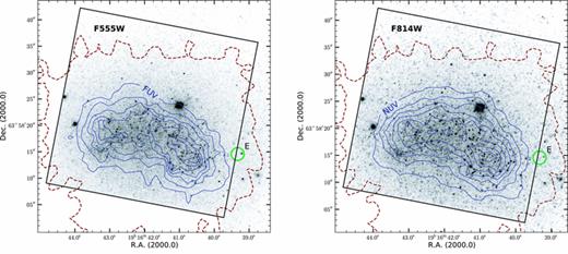
HST WFPC2 images of NGC 6789 in continuum filters F555W and F814W. The solid contours are drawn from FUV and NUV GALEX images, respectively. The dashed contour corresponds to the isophote at 3σ over the level of the sky background of the Palomar/Las Campanas Hα image. The aperture of knot E defined in the Hα image and the rectangle encompassing the FOV of the PC chip of the WFPC2 data are also shown for reference. North is up and east is towards the left-hand side.
The stellar photometric analysis was performed with the hstphot package (Dolphin 2000a). This package is specifically designed for use with HST WFPC2 images and uses a library of tinytim (Krist 1995) undersampled PSFs for different locations of the star on the camera and of the star within the pixel, to centre the star and to find its magnitude, given in the flight system magnitude. The first step was to run the mask task using the HST data quality file (c1f) to mask out the bad pixels and other image defects. The next step was to run crmask for cosmic ray removal. We used a registration factor of 0.5 and σ threshold of 3. It has the capability of cleaning images that are not perfectly aligned, and it can handle images from different filters. After cosmic ray rejection, sets of images of each filter at a common pointing were combined into a single image, using the routine coadd. Since there are two images per pointing, we ended up with three images per filter. The sky computation is made by getsky, which takes all pixels in an annulus around each pixel, determines the sky value and calculates the sky background map. These sky values are used only as a starting guess in the hstphot photometry. The final step requires the use of the hotpixels procedure on each combined image, which uses the result from getsky and tries to locate and remove all hot pixels. This is an important step, since hot pixels can create false detections and can also throw off the PSF solutions.
The main hstphot routine was run on the images in the F555W and F814W bands. This task performs stellar PSF photometry on multiple images from different filters and pointings (providing the dithering pattern, it analyses the dithering image as a whole), including alignment and aperture corrections, as well as PSF modifications to correct for errors of geometric distortion via the Holtzman et al. (1995) distortion correction equations and the 34th row error, noted by Shaklan, Sharman & Pravdo (1995) (see also Anderson & King 1999), and correction for charge transfer inefficiency (Dolphin 2000b). We enabled the determination of a ‘local sky’ value (option 2).
We selected ‘good stars’ from the hstphot output. Object types were classified as good star, possible unresolved binary, bad star, single-pixel cosmic ray or hot pixel and extended object. To ensure selecting high-fidelity point sources, we also used the ‘sharpness’ parameter (absolute value to be ≤0.35), a measure of the quality of the fit (χ2≤ 2.5) and a minimum signal-to-noise ratio of 10 to reject false star detections in regions with structured nebulosity or artefacts. The final number of stars detected in the PC chip with these parameters in both filters is 7410.
To quantify the completeness and systematic uncertainty of the photometry, a grid of artificial stars was generated on a two-dimensional CMD and distributed according to the flux of the images with an artificial star routine provided by hstphot. The parameters of the routine are the minimum and maximum of the measured colour and magnitude. The magnitude steps used were multiple of 0.5, while colour steps are by 0.25. The artificial stars were distributed on the CMD in accordance with the number observed. Approximately 60 000 fake stars were added in each image (at different trials, in order to leave the crowding conditions unaltered) and were given random magnitudes and colours in the observed range. The 50 per cent completeness of the F555W filter is reached at 26.9 mag, while for the F814W filter it is 25.6 mag.
The final CMD of NGC 6789 with typical photometric errors per magnitude bin is shown in Fig. 4.
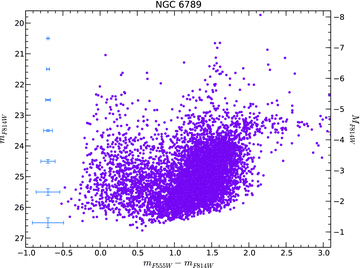
CMD of NGC 6789 with average photometric uncertainties per magnitude bin.
4 DISCUSSION
4.1 Star formation history and stellar populations
Studies to obtain information on the star formation of composite stellar systems have been proved to be very successful (see e.g. Aparicio et al. 1997; Hernandez, Gilmore & Valls-Gabaud 2000; Dolphin 2002). Any SFH recovery method relies on the assumption that a composite stellar population can be considered simply as the combination of SSPs, assigning a certain relative weight to each SSP. The observed CMD is compared with theoretical ones created via Monte Carlo methods for a variety of IMFs, binary fractions, star formation laws etc., extracting the stellar information from isochrones or stellar evolution tracks. Observed and theoretical CMDs are divided into boxes and converted into two-dimensional histograms of stellar density as a function of colour and magnitude (Hess diagrams) and compared using statistical methods.
For the analysis of this work, we used the starfish code7 developed by Harris & Zaritsky (2001). This code was successfully used in a number of cases (e.g. Harris & Zaritsky 2004; Brown et al. 2006; Williams et al. 2007; Harris & Zaritsky 2009; García-Benito et al. 2011). Using determinations of the interstellar extinction, photometric errors and distance moduli, it uses minimization of a chi-squared-like statistics technique to find the linear combination of single-component stellar population models that best fit an observed CMD. The ages and metallicities of the underlying stellar population are characterized by the ages and metallicities of the CMDs included in the best-fitting model, while SFR at each age is provided by the weights given to the CMDs.
The theoretical isochrones chosen for the analysis were those of Marigo et al. (2008),8 for ages in the range of 1 Myr to 14 Gyr. This data set includes models with age bins spaced logarithmically since the CMD changes much more rapidly at young ages than at old ones. We chose the two metallicity values closest to the observed ones (see Section 2.4), namely Z= {0.001, 0.004}. Marigo et al. (2008) provide metallicities in the range 0.0001 ≤Z≤ 0.03. Nevertheless, for the sake of consistency, we selected only the same values that were available for the starlight libraries (Bruzual & Charlot 2003). The photometric error and completeness estimates were taken directly from the results of the artificial star experiments described in Section 3.2. We adopted a Salpeter IMF with a spectral index of −1.35 from 0.1–100 M⊙ (Salpeter 1955). This assumption is likely to be valid since our CMD does not contain stars with masses <1 M⊙. The binary fraction was set to a value of 0.5.
Our reference value for NGC 6789’s distance modulus is (m−M) = 27.80 ± 0.13 ± 0.18, the value reported by Drozdovsky et al. (2001) using the tip of the red giant branch distance method. The Galactic extinction is AV= 0.212, the value provided by Schlegel, Finkbeiner & Davis (1998) extinction maps for an area with radius equal to 5 arcmin around NGC 6789, remarkably close to the reddening value obtained from our spectroscopic data (Section 2.2). Nevertheless, we built a set of models to explore the space of parameters. The SFH recovery is repeated for each point in the grid (m−M) versus AV, and then we built a final  map for the solutions. We explored the space of parameters in steps of 0.01 in distance modulus and extinction. To evaluate the errors of the recovered solutions, we generated a series of synthetic CMDs using the best-fitting SFR and find a correspondence between
  and the confidence level of significance.
Although it is tempting to perform an SFH analysis for each knot, the resulting individual CMDs, taken to be as the stars included inside the defined ellipses (see Fig. 1 and Section 3.1), do not contain enough stars9 and, therefore, the large errors associated with each individual SFH prevent us to draw any conclusion. At any rate, the distribution of stars in each individual CMD is very similar for all the knots. Thus, we use the entire CMD of the galaxy to derive the global SFH.
Fig. 5 shows the overall best-fitting starfish solution for the SFH of NGC 6789, located at (m−M) = 27.83 ± 0.06 and AV= 0.64 ± 0.08, where the errors stand for the 1σ confidence level. The errors in the star formation diagram only allow the consideration of a few main bursts in the SFH. Regarding the lower metallicity (Z= 0.001), the solution shows a few bursty events around 1.6 Gyr and 6–10 Gyr, followed by a more recent burst around 100 Myr and a very young one during the last 12 Myr. As for the higher metallicity (Z= 0.004), only one event between 150 and 300 Myr is clearly seen. Although for the very young stars (<12 Myr) both metallicities present a significant error, we take Z= 0.001 as the metallicity for the youngest event, as derived from the nebular analysis (see Section 2.4). The SFR, according to the starfish results, was stronger around 100 Myr, with a peak of 0.015 M⊙ yr−1.
In the light of these results, we used the age–metallicity solution derived from the CMD as a prior to constrain the libraries of the starlight code, used to fit the spectra of the five knots (see Section 2.2 for more details). In the left-hand panel of Fig. 6 we show the age distribution of the light fraction obtained from starlight for each knot under the constraints mentioned above. Another fitting was carried out without any specific age–metallicity constraint in order to compare it with the results of the first fitting. These are shown in the right-hand panel of Fig. 6. As can be seen, all knots present a very young stellar population, with ages younger than 10 Myr, responsible for the ionization of the gas, combined with other older populations. The presence of these old populations is confirmed with the detection of absorption metal lines of Ca ii K λ3933 Å and Ca ii H λ3968 Å characteristic of old stellar populations, except for knot E, in which these features are marginally detected. The combination of these two different stellar population is also obtained by Pérez-Montero et al. (2010) in a sample of 10 BCDs using the same technique. In terms of mass, more than 80 per cent of it comes from the older population. The estimated total stellar mass and the fraction of the mass of the stellar population with an age younger than 10 Myr with respect to the total mass are given in Table 8. The stellar masses were corrected for aperture effects, with factors calculated using the ratio between the extinction-corrected Hα fluxes measured in the elliptical regions of the photometry and those measured in the extracted long-slit observations for each knot. In the same table, we show the EW(Hβ) values calculated once the contribution of the older stellar populations was removed, in order to use EW(Hβ) to derive the properties of the ionizing stellar population (see Section 4.2). The inner extinctions calculated by starlight for each fit are also listed in the same table. Finally, the results for the non-constrained case are given in the second row for each knot. The values from Table 8 show that fits obtained from non-constrained libraries do not significantly alter some of the properties of the stellar populations, such as the total stellar mass and the correction factor for EW(Hβ), even that some relevant differences appear in the age and metallicity distribution of the resulting SFHs. Therefore, we relied on the general chemical evolution solution derived by starfish to constrain the age–metallicity libraries of starlight. At any rate, the general distribution of the light is similar in both cases. We recall that the CMD SFH (starfish) is derived for the whole galaxy, while the spectra SFH (starlight) is derived for each individual knot.
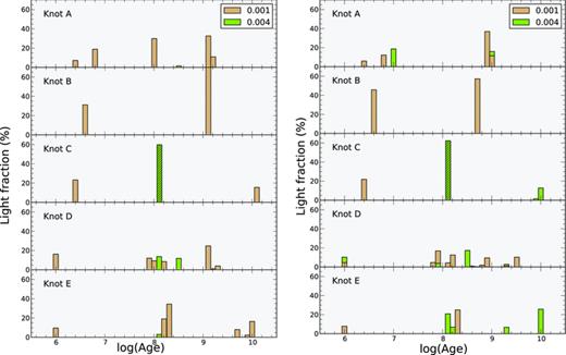
Histograms of the distribution (light fraction) of the best fit derived by starlight for the spectra of the five knots of NGC 6789. The left-hand panel corresponds to the fits using the constrains obtained by the CMD analysis, while the right-hand panel shows the fits using non-constrained age–metallicity libraries.
Properties of the stellar populations as obtained with starlight for each knot of NGC 6789, including the inner extinction, the aperture-corrected total stellar mass, the mass of stars younger than 10 Myr (Mion*) and the EW(Hβ) corrected for the contribution of the older population. The first row for each knot corresponds to the constrained age–metallicity libraries, while the second row is for the unconstrained case.
| ID | A(V) (mag) | logM* | logMion* | EW(Hβ)c (Å) |
| Knot A | 0.4 | 5.34 | 3.69 | 23 |
| 0.4 | 5.35 | 3.81 | 19 | |
| Knot B | 0.3 | 5.26 | 3.16 | 30 |
| 0.7 | 5.22 | 3.68 | 30 | |
| Knot C | 0.7 | 6.00 | 4.03 | 49 |
| 0.6 | 5.97 | 3.95 | 51 | |
| Knot D | 0.5 | 5.42 | 3.79 | 24 |
| 0.5 | 5.51 | 3.66 | 24 | |
| Knot E | 0.7 | 5.16 | 2.71 | 84 |
| 0.5 | 5.21 | 2.47 | 95 |
Less significant is the difference of the fitted spectra between both cases. For these two particular metallicities, the variation of the intensity of the first four Balmer lines on the residual spectra for each knot is well within the observational errors when using one or the other case. The change of the age–metallicity distribution in the libraries only affects significantly in these two particular cases to the SFH in the assignments of the metallicity of the stellar populations, but the overall derived age distribution is very similar.
Regarding the extinction, we find some discrepancies between the values found by starlight and those derived using Balmer decrements. However, the average extinction value for all knots (0.52 ± 0.16) is very close to the CMD best-fitting value given by starfish (0.64 ± 0.08). It should be noted, though, that in principle it is not expected to find the same values in the gas and the stellar population.
4.2 Ionizing stellar populations and photoionization models
Among the properties of the young ionizing populations that can be derived from optical spectroscopy are their stellar masses and ages. The former can be derived from the Hα luminosity and EW(Hβ) (e.g. Díaz 1998). The Hα luminosity can also be used to estimate the SFR and the mass of ionized hydrogen. The age can be estimated by using the EW(Hβ) as compared to sequences of evolutionary synthesis models. In our case, the contamination of the older underlying population to the Hβ continuum was removed by using the analysis made with starlight. As can be seen in Table 8, these corrections are quite different between the knots, going from a 3 per cent in the case of knot B to a 42 per cent in the case of knot E.
 . Thus, this implies that dust absorption could be mainly responsible for the disagreement between expected and observed EW(Hβ). Thus, both L(Hα) and EW(Hβ) must be corrected using the dust absorption factor (fd) before the derivation of the properties of the ionizing cluster. This correction must be done even after the extinction correction, because it corresponds to the fraction of ionizing photons absorbed by the dust and, therefore, not absorbed and re-emitted by the gas:
Properties of the individual knots derived from tailored photoionization models compared with the observed values.
| NGC 6789-A | NGC 6789-B | NGC 6789-C | NGC 6789-D | NGC 6789-E | ||||||
| Mod. | Obs. | Mod. | Obs. | Mod. | Obs. | Mod. | Obs. | Mod. | Obs. | |
| log L(Hα) (erg s−1) | 37.32 | 37.23 ± 0.02 | 37.34 | 37.34 ± 0.02 | 37.51 | 37.50 ± 0.03 | 37.18 | 37.17 ± 0.02 | 37.03 | 37.02 ± 0.01 |
| Radius (pc) | 7 | 30 | 33 | 34 | 22 | 37 | 10 | 36 | 5 | 21 |
| FUV–NUV (mag) | 0.17 | 0.14 ± 0.16 | 0.28 | 0.28 ± 0.19 | 0.30 | 0.31 ± 0.22 | 0.22 | 0.03 ± 0.18 | 0.10 | 0.06 ± 0.04 |
| I([O ii]/I(Hβ) | 2.30 | 2.34 ± 0.15 | 3.33 | 3.16 ± 0.20 | 2.35 | 2.51 ± 0.16 | 3.05 | 3.14 ± 0.20 | 1.09 | 1.06 ± 0.04 |
| I([O iii]/I(Hβ) | 3.82 | 3.76 ± 0.17 | 1.47 | 1.48 ± 0.07 | 3.45 | 3.44 ± 0.15 | 1.72 | 1.73 ± 0.08 | 2.30 | 2.26 ± 0.20 |
| 12+log(O/H) | 7.93 | 7.84 ± 0.04 | 7.82 | 7.93 ± 0.10 | 7.79 | 7.81 ± 0.05 | 7.77 | 7.90 ± 0.12 | 7.64 | 7.80 ± 0.18 |
| −EW(Hβ (Å) | 21 | 23 | 30 | 30 | 48 | 49 | 29 | 24 | 80 | 84 |
| Age (Myr) | 5.4 | – | 4.2 | – | 3.5 | – | 5.2 | – | 3.9 | – |
| Dust-to-gas ratio | 0.026 | – | 0.34 | – | 0.12 | – | 0.15 | – | 0.015 | – |
| Abs. factor (fd) | 5.34 | – | 7.28 | – | 8.21 | – | 4.37 | – | 2.23 | – |
The assumptions taken for the models described above may be an oversimplification as they do not take into account the three-dimensional structure of the ionized gas and the dust. Besides, we cannot take as input parameter the dust-to-gas ratio of this galaxy and possible uncertainties related with the adopted synthesis stellar atmospheres can affect the final result.
As can be seen, the observed properties are generally well fitted by the models, by assuming different geometries and dust-to-gas ratios without noticeably changing the derived metallicity of the gas. According to our results, fd correlates better with the FUV–NUV index than that with the reddening constant derived from the Balmer decrement in the optical spectra. For instance, knot C has the highest fd with the lowest c(Hβ) and, in contrast, knots A and E have the lowest fd and the highest c(Hβ). This could be indicative of a complex inner dust structure which is not well traced by the reddening constant derived from the Balmer decrement. Regarding the cluster ages, our results indicate that all knots have an ionizing cluster in a range of ages between 3.5 Myr for knot C and 5.4 Myr for knot A. The youngest cluster appears in knot C, although knot E, which has a very low fd correction, has the lowest EW(Hβ). The age sequence in the studied knots does not correspond to any specific spatial order.
The total masses of the ionizing clusters were also derived by using the number of ionizing photons and the ages obtained from the respective cloudy models and the starburst99 libraries of the corresponding synthesis cluster atmospheres. These are listed in Table 10. As can be seen, the stellar masses of the bursts in the four first knots are quite similar, while knot E has the lowest value. These masses are in agreement within 0.3 dex with the masses derived for the younger stellar population using the fitting to the optical spectrum made with starlight (Table 8).
Properties of ionizing stellar populations in the knots as derived using the Q(H0) value obtained from the photoionization models.
| ID | log Q(H 0) (erg s−1) | log Mburst (M⊙) | log M(H ii) (M⊙) | log SFS (M⊙) | SFR (10−3 M⊙ yr−1) |
| Knot A | 49.94 | 3.82 | 3.45 | 4.34 | 1.04 |
| Knot B | 50.09 | 3.65 | 3.60 | 4.32 | 1.47 |
| Knot C | 50.31 | 3.69 | 3.82 | 4.54 | 2.44 |
| Knot D | 49.69 | 3.52 | 3.20 | 4.09 | 0.59 |
| Knot E | 49.25 | 2.73 | 2.76 | 3.48 | 0.21 |
| NGC 6789a | 51.49 | - | 5.00 | 5.89 | 36.97 |
aValues derived from the Hα image, not corrected for extinction.
It is known that the SFR determined from Hα is sensitive to several uncertainties, as those related with the extinction and the assumed IMF. Besides, not always all the ionizing photons are absorbed, the escape fraction of ionizing radiation from individual H ii regions (in nearby galaxies) being between 15 and 50 per cent (Kennicutt 1998). We applied the calibration by Otí-Floranes & Mas-Hesse (2010),10 which makes a distinction between instantaneous burst (IB) and extended burst (EB). We used our extinction and dust-absorption corrected Hα luminosity (except for the value of the whole galaxy) and a Salpeter IMF in the range of 0.1–100 M⊙ as input. For the IB case, the value given by the calibration is the SFS. The SFS values in Table 10 were calculated using the age provided by the calibration, namely 4, 5 and 6 Myr, closest to the age estimated from the photoionization models. According to this calibration, the mass of gas transformed in stars during the actual burst in each knot is of the order of tens of thousands of solar masses, except for knot E, which is one order of magnitude lower.
We provide as well the SFR, for the EB case (continuous star formation), as a reference value. Regarding the SFR of the whole galaxy, the value estimated by means of the Hα flux is slightly higher than the peak obtained from the CMD (see Fig. 5). The SFR for BCDs spans from a few 10−3 to several times 101 M⊙ yr−1 (Hopkins, Schulte-Ladbeck & Drozdovsky 2002; Zhao, Gu & Gao 2011), showing that NGC 6789 is not of a particularly high value.
Although our models are able to reproduce much of the observational information both in the optical and the UV, some of their limitations must be taken into account. It is possible that EW(Hβ) could be modified owing to great fractions of leaked photons. However, comparing the mass of ionized gas in this galaxy [log(M/M⊙) ∼ 5, see Table 10] with the mass of neutral hydrogen does not support this scenario, but taking into account the oversimplified geometry of our models, it cannot be ruled out completely. In this sense, as the long slit does not cover entirely the gas emission from the knots, EW(Hβ) are lower limits. Nonetheless, the aperture factors derived from the direct comparison with the Hα image do not lead to a satisfactory solution.
Larger dust-to-gas ratios and fd than typical values for H ii regions with larger metallicity (e.g. Inoue 2001) were derived by the models in all knots in order to fit the observed EW(Hβ) and FUV–NUV colours. However, these values cannot be taken as representative of the whole galaxy but only for the analysed star-forming knots, considering that the fraction of ionized-to-neutral gas is quite small, as mentioned above, and that this galaxy does not present a very high infrared luminosity (i.e. it does not appear in the IRAS catalogue). We have run other sets of models with standard dust-to-gas ratio values, but they do not fit the observables mentioned above. The dust-to-gas ratios could be considerably decreased by assuming different geometries of the gas and dust inside the H ii regions, but this approach is beyond the scope of this work.
Finally, our results about the masses and ages of the ionizing clusters must be used only as a guiding signpost, as the involved masses range in a regime (∼104 M⊙) where stochastic fluctuations in the IMF can be important (Cerviño & Valls-Gabaud 2003; Cerviño & Luridiana 2006). In this sense, IMF sampling effects (Pflamm-Altenburg, Weidner & Kroupa 2007, 2009) can also alter our results, as there can be a lower number of massive stars than those expected for the mass range of these knots.
4.3 Densities, temperatures and chemical abundances
The derived densities, both for [S ii] and [O ii], are very similar for the first four knots, being lower than 100 cm−3. Interestingly, knot E, located in the outskirts of the galaxy, shows a density twice that of the knots located in the central part of the galaxy. At any rate, these densities are typical of low-density environments found in BCDs.
Regarding electron temperatures, T([O iii]) was measured in the five knots, with errors which depend on the quality of the spectrum in each knot going from 3 per cent in knot A up to 13 per cent in knot E. The first four star-forming regions show very similar [O iii] temperatures, all within a relatively narrow range, between 13 000 and 14 300 K, while knot E has a lower temperature by about 2000 K. To our knowledge, there is no previous report on T([O iii]) for this galaxy in the literature.
T([O ii]) was also measured in three of the knots (B, C and E) and it was estimated in the other two knots by means of relations between these temperatures and the measured value of T([O iii]). The knot C, which is the brightest in Hα, has in average higher temperatures.
We derived oxygen, nitrogen, sulphur, neon and argon total abundances in all the studied knots by taking the ionic abundances calculated in Section 2.4 and the ICFs estimated in our tailored photoionization models. As in the case of temperatures, no other direct abundance determination exists in the literature for this galaxy. In average, NGC 6789 shows an oxygen abundance characteristic of the low values found in strong line BCDs, with values in all knots in the range of 12+log(O/H) = 7.80–7.93, which is compatible with a similar abundance in all knots taking into account the errors. This behaviour, i.e. showing different star-forming knots within a BCD close abundance values (i.e. <0.2 dex), is also found in other objects using both long-slit spectroscopy (Papaderos et al. 2006; Cairós et al. 2009; Pérez-Montero et al. 2009; Hägele et al. 2011) and integral field spectroscopy (Kehrig et al. 2008; Pérez-Montero et al. 2011), or in H ii complexes in spiral galaxies with a similar spatial scale (Kennicutt, Bresolin & Garnett 2003; García-Benito et al. 2010).
Since nitrogen and oxygen have different nucleosynthetic origins, their ratio is related to the chemical history of galaxies. Primary nitrogen synthesis is thought to occur in intermediate-mass stars in the CNO process during hydrogen burning which is hence independent of the initial heavy-element abundances, while secondary nitrogen production is expected to be produced in stars of all masses (Vila Costas & Edmunds 1993). At low metallicity, most part of nitrogen has a primary origin and a constant log(N/O) ratio is observed. However, the N/O values found in the studied knots of NGC 6789 range in an interval (from −1.38 to −1.26) sensibly higher than the observed values for other BCDs or low-metallicity dwarf irregular galaxies (Izotov & Thuan 1999; Vílchez & Iglesias-Páramo 2003; van Zee & Haynes 2006; Pérez-Montero & Contini 2009), which is around log(N/O) ≈−1.6. In the case of knot C, this ratio is even higher, with a value of −1.07. The cause of these relatively high N/O can be partially found in the corresponding ICFs derived by the models as the total nitrogen abundances derived from the assumption N/O ≈ N+/O+ give lower N/O values in knots A [log(N/O) =−1.41] and C [log(N/O) =−1.34], although still higher within the errors than the typical N/O value for BCDs.
On the other hand, several causes are cited in the literature to explain this overabundance of nitrogen in low-metallicity environments [e.g. the pollution of the interstellar medium (ISM) by Wolf–Rayet stellar winds], but it is especially indicative in this case that we found this overabundance in the five knots, which present different evolutionary and excitation properties. Therefore, the high N/O is apparently related with some other process affecting all the ISM of the galaxy. The fall of pristine gas in the galaxy could explain the N/O overabundance (Köppen & Hensler 2005) and, at the same time, the triggering of the star formation in different places of the galaxy with very short time intervals between them.
The ratio of the alpha elements, sulphur, neon and argon, to oxygen should be constant and show no dependence on the oxygen abundance, since all are products of α-processes in the same massive stars that make oxygen. The derived log(S/O) ratios range between −1.64 and −1.41 in the four first knots and it is sensibly higher in knot E, but in this knot the derivation is much more uncertain as no [S iii] was measured. Although the ratio seems to increase from knot A to D, the average error (∼0.18) prevents us from drawing any conclusion about the homogeneity.
Regarding the logarithmic Ne/O ratio, knots A and C show the same value, −0.70, while for the rest of the knots the mean value is −0.94, with an average error of 0.07 dex for A and C and 0.20 dex for B, D and E.
The Ar/O ratios found, in the range −2.28 to −2.06, show a very similar value for all knots, taking 0.17 dex as the average error (ranging from 0.09 up to 0.22 dex).
Finally, the derived helium abundances are the same for all five knots of NGC 6789 within observational errors, and similar to the values found for other BCDs (Izotov & Thuan 2004; Hägele et al. 2008).
5 CONCLUSIONS
In this paper, we present resolved stellar, Hα and GALEX photometry, from different data archives, and WHT-ISIS optical spectroscopy of the five brightest star-forming knots of the nearest BCD galaxy NGC 6789 in order to study their SFH and metallicity.
The spectroscopic observations of NGC 6789 were taken using the ISIS double-arm spectrograph attached to the 4.2-m WHT, which allowed the simultaneous analysis of the spectra, covering from 3650 up to 7500 Å. From the long-slit spectra, we extracted and performed a detailed analysis of the five main star-forming knots of the galaxy. Thanks to the measure of the [O iii] electron temperature in all knots and the measure of T([O ii]) in three of them, we provide ‘direct method’ abundances for oxygen, nitrogen, sulphur, neon and argon, not reported previously in the literature. Our analysis indicates that this galaxy is metal-poor (12+log(O/H) in the range of 7.80–7.93) and chemically homogeneous, with quite similar values as of the studied species in all knots. At same time, all the knots present values of N/O which are higher than those expected for the metal regime of this galaxy.
We used optical data obtained from the HST archive to derive the SFH of NGC 6789 by means of the classical method of CMD reconstruction. We used the derived SFH in the program starlight to fit the optical spectrum and we compared these results with another non-constrained case. We corrected the emission-line measures from absorption and derived the total stellar masses for each knot. Although the SFH obtained from the CMD is not foreseen by starlight in the non-constrained case, we checked that the total stellar mass and the ratio of older and younger stellar populations are not noticeably affected by the assumed SFH. Anyway, whenever possible, the extension of such studies for objects for which simultaneous resolved stellar photometry and optical spectroscopy are available will provide a much more accurate constraint to the age–metallicity extinction degeneracy of these galaxies, as well as the comparison between nebular and stellar properties.
Finally, the ages and masses of the bursts of star formation in each knot were derived using cloudy-tailored photoionization models to fit the optical and UV photometric properties and the observed emission-line ratios and corrected Hβ equivalent widths. We found that dust absorption factors correlate much better with the GALEX FUV–NUV colour index than with the reddening constants derived from the Balmer decrement, indicating a very complex inner dust extinction structure. The models predict for all knots instantaneous bursts with ages in the range between 3 and 6 Myr. These ages do not follow any spatial trend in the galaxy image, so they are possibly related with the distribution of the galaxy in the line of sight. The dust-absorption corrected Hα fluxes were used to derive accurate SFRs for the individual knots.
The combination of several observational and model techniques leads to a better and auto-consistent study of NGC 6789. The derivation of a non-typical metallicity evolution using a CMD allows the use of the SFH to the subtraction of the older stellar population using spectral fitting to the optical spectrum with starlight. This information, together with the derivation of accurate physical properties and ionic chemical abundances pointing to similar low O/H and high N/O ratios in all knots, allows the application of photoionization models that predict dust-absorption factors fitting the GALEX colour indices and the derivation of ages (instantaneous bursts in the range of 3–6 Myr).
RG-B acknowledges support from the China National Postdoc Fund Grant No. 20100480144 and MICINN AYA2010-15081. This work has been partially supported by projects AYA2007-67965-C03 and AYA2010-21887-C04 of the Spanish National Plan for Astronomy and Astrophysics. The WHT is operated on the island of La Palma by the ING in the Spanish Observatorio del Roque de los Muchachos of the Instituto de Astrofísica de Canarias. We thank the Spanish allocation committee (CAT) for awarding observing time. We also thank Armando Gil de Paz for allowing the study of B, R and Hα images of NGC 6789 in the Palomar/Las Campanas Atlas of Blue Compact Galaxies. We thank Roberto Cid Fernandes and the people of the starlight Project Team (UFSC, Brazil) for making the starlight code available. We acknowledge fruitful discussions with Enrique Pérez and Ricardo Amorín. We also thank an anonymous referee for very useful comments that improved the presentation of the paper.
Footnotes
The central regions show a very complex structure with several centers of star formation and very irregular (i) isophotes, while the outer isophotes are elliptical (E).
iraf, the Image Reduction and Analysis Facility, is distributed by the National Optical Astronomy Observatories, which is operated by the Association of Universities for Research in Astronomy, In. (AURA) under cooperative agreement with the National Science Foundation (NSF).
The starlight project is supported by the Brazilian agencies CNPq, CAPES and FAPESP and by the France–Brazil CAPES/COFECUB programme.
Z⊙= 0.0122.
From several fitting experiments using other libraries, it is found that the resolution of the SSP spectra is a critical factor for starlight in order to fit the absorption lines.
c(Hβ) = 0.4656 A(V), using Cardelli et al. (1989) and RV= 3.1.
Available at http://www.noao.edu/staff/jharris/SFH/
Available at http://stev.oapd.inaf.it/cgi-bin/cmd/
Specially knot E, part of which falls outside the PC FOV.
Their web tool can be found at http://www.laeff.cab.inta-csic.es/research/sfr/
REFERENCES
