


Abstract
We present a new 400-ks Chandra X-ray observation of the merging galaxy cluster Abell 2146. This deep observation reveals detailed structure associated with the major merger event including the Mach number M= 2.3 ± 0.2 bow shock ahead of the dense, ram pressure stripped subcluster core and the first known example of an upstream shock in the intracluster medium (ICM) (M= 1.6 ± 0.1). By measuring the electron temperature profile behind each shock front, we determine the time-scale for the electron population to thermally equilibrate with the shock-heated ions. We find that the temperature profile behind the bow shock is consistent with the time-scale for Coulomb collisional equilibration and the post-shock temperature is lower than expected for instant shock heating of the electrons. Although like the Bullet cluster the electron temperatures behind the upstream shock front are hotter than expected, favouring the instant heating model, the uncertainty on the temperature values is greater here and there is significant substructure complicating the interpretation. We also measured the width of each shock front and the contact discontinuity on the leading edge of the subcluster core to investigate the suppression of transport processes in the ICM. The upstream shock is ∼440 kpc in length but appears remarkably narrow over this distance with a best-fitting width of only 6+5−3 kpc compared with the mean free path of 23 ± 5 kpc. The leading edge of the subcluster core is also narrow with an upper limit on the width of only 2 kpc separating the cool, multiphase gas at 0.5–2 keV from the shock-heated surrounding ICM at ∼6 keV. The strong suppression of diffusion and conduction across this edge suggests a magnetic draping layer may have formed around the subcluster core. The deep Chandra observation has also revealed a cool, dense plume of material extending ∼170 kpc perpendicular to the merger axis, which is likely to be the disrupted remnant of the primary cluster core. This asymmetry in the cluster morphology indicates the merger has a non-zero impact parameter. We suggest that this also explains why the south-western edge of the subcluster core is narrow and stable over ∼150 kpc in length, but the north-eastern edge is broad and being stripped of material.
1 INTRODUCTION
Galaxy clusters are formed through mergers of smaller subclusters and groups, which collide at velocities of several thousand km s−1. The total kinetic energy of these mergers can reach 1064 erg, a significant fraction of which is dissipated by large-scale shocks and turbulence over the merger lifetime (for a review see Markevitch & Vikhlinin 2007). Shocks and turbulence generated by the merger are also expected to amplify magnetic fields in the cluster and accelerate relativistic particles. These non-thermal phenomena have been revealed through the detection of Mpc-scale synchrotron radio haloes (for recent reviews see Feretti & Giovannini 2008; Ferrari et al. 2008) and inverse-Compton hard X-ray emission (Fusco-Femiano, Landi & Orlandini 2005; Rephaeli, Gruber & Blanco 1999, but see also Wik et al. 2009). The combination of X-ray and gravitational lensing studies of merging clusters has also produced compelling evidence for dark matter (e.g. Clowe, Gonzalez & Markevitch 2004; Bradač et al. 2006; Clowe et al. 2006) and constraints on the dark matter self-interaction cross-section (e.g. Randall et al. 2008).
Chandra’s subarcsecond angular resolution revealed sharp X-ray surface brightness edges in merging systems. These edges correspond to cold fronts or contact discontinuities between regions of gas with different entropies (Markevitch et al. 2000; Vikhlinin, Markevitch & Murray 2001a; Markevitch & Vikhlinin 2007), and shock fronts driven by infalling subclusters. However, whilst cold fronts are also found in relaxed clusters and are common in cluster cores (e.g. Owers et al. 2009), there are only a few confirmed detections of shock fronts with a sharp density edge and an unambiguous temperature jump (the Bullet cluster, Markevitch et al. 2002; Abell 520, Markevitch et al. 2005; two in Abell 2146, Russell et al. 2010; Abell 754, Macario et al. 2011; and Abell 2744, Owers et al. 2011). These surface brightness edges are key observational tools for studying merging systems and provide currently the only method for measuring the bulk velocities of the gas in the plane of the sky and determining the velocity and kinematics of the merger.
Detailed observations of shock fronts and cold fronts have been used to probe the relatively unknown transport processes in the intracluster medium (ICM). Markevitch (2006) used a deep observation of the bow shock in the Bullet cluster to produce the first measurement of the electron–ion thermal equilibration time-scale in the ICM and determine that the time-scale is likely to be shorter than the Coulomb collisional time-scale (e.g. Fox & Loeb 1997; Markevitch 2006; Markevitch & Vikhlinin 2007). This exciting result suggests a heating process that operates faster than Coulomb collisions could be operating in the magnetized ICM (e.g. Schekochihin et al. 2005; Schekochihin et al. 2008). Observations of the sharp temperature and density jumps at cold fronts suggest that thermal conduction and diffusion are strongly suppressed across these edges (e.g. Ettori & Fabian 2000). A detailed study of the cold front in Abell 3667 found that the width of the density jump is smaller than the Coulomb mean free path in the ICM (Vikhlinin et al. 2001a). This edge also appears sharp and stable within a large sector of ±30° around the symmetry axis suggesting that hydrodynamic instabilities are also suppressed. The flow of the ambient ICM around the dense subcluster core will stretch initially tangled magnetic field lines to form a draping layer with a magnetic field parallel to the front (Vikhlinin, Markevitch & Murray 2001b; Vikhlinin & Markevitch 2002; Asai, Fukuda & Matsumoto 2005; Lyutikov 2006). This magnetic draping layer could provide a stabilizing mechanism and will suppress transport processes across the edge. The long, straight edges of the bullet subcluster in the Bullet cluster also suggest a strong suppression of turbulence by such a stabilizing magnetic layer (Markevitch 2006).
The galaxy cluster Abell 2146 (z= 0.234; Struble & Rood 1999; Böhringer et al. 2000) is a spectacular merging system with two large Mach number M∼ 2 shock fronts (Russell et al. 2010). The X-ray morphology suggests a recent collision, 0.1–0.3 Gyr ago, where a subcluster containing a dense cool core has passed through the centre of a primary cluster. The subcluster is driving a bow shock through the ICM and is trailed by a tail of ram pressure stripped material. An upstream shock is also observed to be propagating in the opposite direction through the outskirts of the primary cluster. Canning et al. (2011) used the line-of-sight velocity difference between the subcluster and primary cluster brightest cluster galaxies (BCGs) with the shock velocities to estimate that the merger axis is inclined at only ∼17° to the plane of the sky. This conclusion is also supported by the sharp surface brightness edges of the bow and upstream shock fronts, which would be smeared by projection for a larger angle to the line of sight. Abell 2146 appears to have undergone a simple merger between two smaller clusters, viewed close to side-on, and therefore has a remarkably similar structure to the Bullet cluster (Markevitch et al. 2002; Markevitch 2006).
In this paper, we present results from a deep 400-ks Chandra observation of Abell 2146 studying the transport processes in the ICM. In Section 2, we discuss the Chandra data reduction, analyse the X-ray morphology and present maps of the ICM temperature, density and metallicity. In Section 3, we analyse the shock fronts in detail and compare the post-shock electron temperature profiles behind the bow and upstream shock fronts with models for instant and collisional electron–ion equilibration. In Section 4, we study the ram pressure stripping of the subcluster core and study the suppression of diffusion and conduction across the leading edge of the subcluster core. We assume H0=70 km s−1 Mpc−1, Ωm= 0.3 and  , translating to a scale of 3.7 kpc arcsec−1 at the redshift z= 0.234 of Abell 2146. All errors are 1σ unless otherwise noted.
2 Chandra DATA ANALYSIS
2.1 Data reduction
Abell 2146 was observed with the Chandra ACIS-I detector for a total of 377 ks split into eight separate observations between 2010 August and October (Table 1). These new observations were analysed together with the archival ACIS-S observations taken in 2009 April (Russell et al. 2010; Table 1). All data sets were reprocessed with ciao v4.3 and caldb v4.4.0 provided by the Chandra X-ray Center. The level 1 events files were reprocessed to apply the latest gain and charge transfer inefficiency correction and then filtered to remove photons detected with bad grades. The improved background screening provided by VFAINT mode was also applied. Background light curves were extracted from the level 2 events files of neighbouring chips for observations on ACIS-I and from ACIS-S1 for observations on ACIS-S3. The background light curves were filtered using the lc_clean script1 provided by M. Markevitch to identify periods affected by flares. There were no major flares in any of the observations of Abell 2146 producing a final cleaned exposure of 418 ks.
Details of the Chandra observations analysed in this paper.
| Date | Obs. ID | Aim point | Exposure (ks) | Cleaned (ks) |
| 2009 April 29 | 10888 | S3 | 6.4 | 6.4 |
| 2009 April 30 | 10464 | S3 | 35.7 | 35.7 |
| 2010 August 10 | 13020 | I0 | 41.5 | 41.5 |
| 2010 August 12 | 13021 | I0 | 48.4 | 48.4 |
| 2010 August 19 | 13023 | I1 | 27.7 | 27.7 |
| 2010 August 20 | 12247 | I1 | 65.2 | 65.2 |
| 2010 September 8 | 12245 | I2 | 48.3 | 48.3 |
| 2010 September 10 | 13120 | I2 | 49.4 | 49.4 |
| 2010 October 4 | 12246 | I3 | 47.4 | 47.2 |
| 2010 October 10 | 13138 | I3 | 49.4 | 48.4 |
The cleaned events files were then reprojected to match the position of the obs. ID 12245 observation. Fig. 1 shows the total combined image produced by summing images in the 0.3–7.0 keV energy band extracted from each individual reprojected data set. This summed image was then corrected for exposure variation by dividing by the summed 1.5 keV monochromatic exposure maps created for each data set. Point sources were identified using the ciao algorithm wavdetect, visually confirmed and excluded from the analysis using elliptical apertures with radii set to five times the measured point spread function width (Freeman et al. 2002).
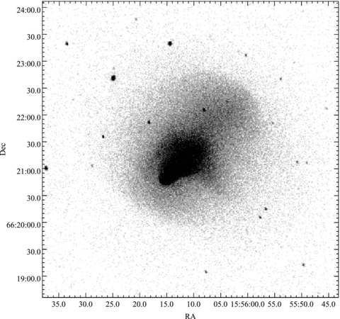
Raw counts image of Abell 2146 in the 0.3–7.0 keV energy band. The image has been binned by a factor of 2.
Standard blank-sky backgrounds were extracted for each chip in each observation, processed identically to the events file and reprojected to the corresponding sky position. Each blank-sky background was normalized to match the count rate in the 9.5–12 keV energy band in the observed data set. This correction was less than 10 per cent for each data set. The normalized blank-sky background events files for each chip in an observation were then split to ensure each had the same ratio of exposure time to observed exposure time. These were then summed together to produce background events files which covered all chips in each observation. By matching to the hard X-ray background count rate, we may over- or under-estimate the soft component of the X-ray background. The normalized blank sky background data sets were tested by comparison with observed background spectra extracted from source-free regions of the chips. We found that the normalized blank sky backgrounds were a close match to the observed background over the whole energy band. Total blank-sky background images combining all of the observations were generated in a similar way to the total images as detailed above.
2.2 Imaging analysis
Fig. 2 (upper left-hand panel) shows an exposure-corrected image of the cluster X-ray emission produced by combining all of the individual Chandra observations. The cluster gas is extended along the merger axis, north-west (NW) to south-east (SE), and the bright, dense core of the subcluster is offset from the centre and being stripped of its material by ram pressure in the collision. The X-ray morphology suggests a major merger where the subcluster has recently passed through the centre of the primary cluster. There is no obvious surface brightness peak associated with a primary cluster core. The primary cluster may not have originally had a dense core or it could have been significantly disrupted in the collision with the subcluster core. The subcluster is observed soon after core passage when it has emerged from the primary core and is travelling towards the SE. Fig. 2 (lower right-hand panel) shows a Subaru R-band image of the galaxy distribution (King et al., in preparation). The distribution of red-sequence galaxies appears to separate into two groups, corresponding to the locations of the subcluster and the primary cluster, which supports the interpretation of a major merger (Canning et al. 2011).
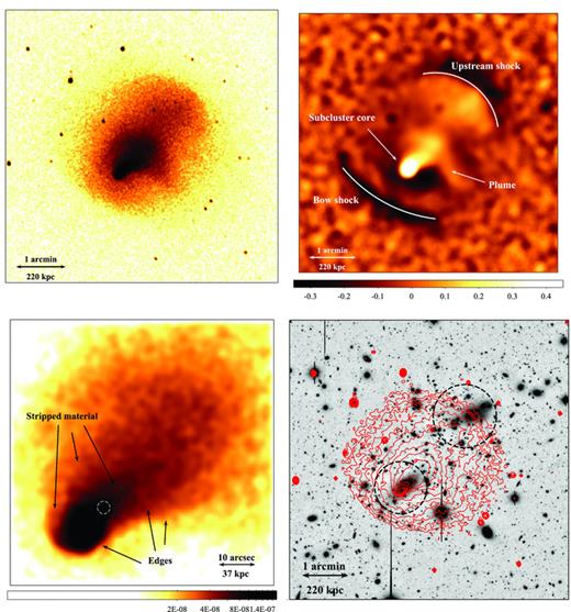
Upper left-hand panel: exposure-corrected image in the 0.3–7.0 keV energy band smoothed with a two-dimensional Gaussian σ= 1.5 arcsec (north is up and east is to the left). Upper right-hand panel: unsharp-masked image created by subtracting images smoothed by two-dimensional Gaussians with σ= 5 and 20 arcsec and dividing by the sum of the two images. Point sources were removed before unsharp masking. Note that a point source has been removed at the NE end of the bow shock. Lower left-hand panel: same as the upper left-hand panel but showing the subcluster core (in units of photons cm−2 s−1 pixel−1). The AGN nucleus is marked by the white dashed circle. Lower right-hand panel: Subaru R-band image of the galaxy distribution in Abell 2146 with the X-ray gas contours overlaid. Concentrations of galaxies are marked with the dashed circles.
The two shock fronts, reported in Russell et al. (2010), are clearly visible in the unsharp-masked image (Fig. 2, upper right-hand panel) as surface brightness edges to the SE and NW. The SE edge corresponds to the bow shock, which has formed ahead of the subcluster core, and can now be traced over ∼500 kpc in length. The NW surface brightness edge corresponds to the upstream shock, which has formed in the wake of the subcluster’s passage through the primary cluster core and is travelling in the opposite direction to the bow shock (Russell et al. 2010). The upstream shock is visible over ∼440 kpc in length and appears to have greater curvature compared to the bow shock. Note that in Fig. 2 (upper right-hand panel) a point source has been removed at the north-eastern (NE) end of the bow shock, which has the effect of increasing the apparent curvature of the shock front. There is no obvious second surface brightness peak corresponding to the primary cluster core and this may have been completely disrupted in the collision with the subcluster.
The deeper Chandra observations have also now revealed the complex structure of the cool, dense subcluster core and the ram pressure stripped tail. Whilst the leading edge of the core is smooth, narrow and roughly spherical, there is a clear difference between the NE and SW edges of the tail (Fig. 2, lower left-hand panel). The SW edge appears sharp and narrow over a distance of ∼40 arcsec. In comparison, the NE edge is poorly defined; it appears broader and disrupted, suggesting that the interface with the ambient medium has become turbulent here and instabilities could be developing. There is also an extended plume of emission to the SW from the subcluster tail, ∼45 arcsec in length, which is perpendicular to the merger axis. These features are discussed further in Section 4.
Fig. 3 shows the subcluster core in detail and the location of the BCG immediately behind the X-ray peak. The deep Chandra data set confirms the detection of a hard X-ray (4–7 keV) point source, at the 3σ level, coincident with a radio point source detected in VLA 1.4-GHz archival data (NRAO/VLA Archive Survey) and observations with the AMI Large Array at 16 GHz (AMI Consortium: Rodríguez-Gonzálvez et al. 2011). Also, Spitzer observations of the BCG by Quillen et al. (2008) suggest that there is a strong contribution to the infrared (IR) emission from an active galactic nucleus (AGN). This radio and X-ray point source likely corresponds to an AGN at the centre of the BCG. However, it was difficult to determine the flux as the nucleus is superimposed on a bright, dense filament of gas, which is detected in soft X-rays with Chandra, but also in Hα and [N ii] (Canning et al. 2011). We extracted the AGN source counts in a region of 2 arcsec radius and subtracted the cluster emission using a neighbouring region to the SE from 2.5 to 5 arcsec radius, which lay on the dense gas filament. For the energy band 2–7 keV, the point source was detected as 210 ± 30 counts above the background cluster emission. Assuming a power-law model with photon index Γ= 2 and Galactic absorption of  (Kalberla et al. 2005), we estimated the point source luminosity in the energy range 2–10 keV to be
  .
.
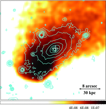
Exposure-corrected image of the subcluster core in the 0.3–7.0 keV energy band smoothed with a two-dimensional Gaussian σ= 1 arcsec (north is up and east is to the left; in units of photons cm−2 s−1 pixel−1). The blue contours were produced from the HSTF606W archival image of the galaxies (blue), including the BCG, and the white cross shows the location of the VLA 1.4-GHz point source marking the nucleus (NRAO/VLA Archive Survey).
2.3 Spatially resolved spectroscopy
2.3.1 Contour binning maps
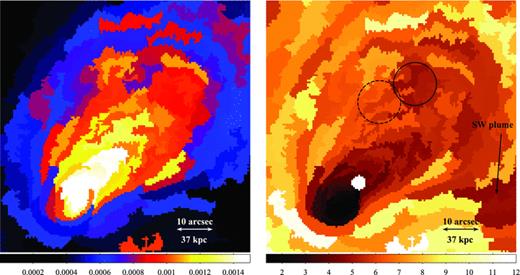
We used spatially resolved spectroscopy techniques to produce detailed maps of the projected gas properties (Fig. 4). The central ∼4 × 4 arcmin2 was divided into regions using the contour binning algorithm (Sanders 2006), which traces the surface brightness variations to generate the spatial bins. For the temperature and normalization maps, regions with a signal-to-noise ratio (S/N) of 32 (∼1000 counts) were chosen. The length of the regions was restricted to be at most two and a half times their width. For each Chandra observation, we extracted a spectrum from each of the regions, subtracted the background spectrum and generated appropriate responses and ancillary responses. The spectra were grouped to contain a minimum of 20 counts per spectral channel and restricted to the energy range 0.5–7 keV. We summed together spectra and background spectra for a particular region for observations on the same chip, as the roll angles are also comparable in each case. The response files were also averaged together, weighting by the fraction of the total counts in each observation. Each total spectrum was fitted in xspec v12 (Arnaud 1996) with an absorbed mekal model. The absorption was fixed to the Galactic value  (Kalberla et al. 2005) and the redshift was fixed to 0.234. The C-statistic was minimized in the spectral fitting (Cash 1979). The errors are approximately ∼6 per cent in emission measure and ∼15 per cent in temperature. However, the error in temperature drops to less than 10 per cent in the subcluster core, where the temperature falls below 2 keV and the Fe L line emission improves temperature diagnostics. In addition, temperatures over 10 keV are poorly constrained by the energy range of Chandra and the errors increase to ∼30 per cent in these bins.
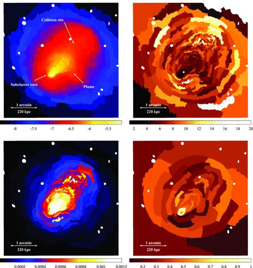
Upper left-hand panel: projected emission measure per unit area map (units are log10 cm−5 arcsec−2). The emission measure is the xspec normalization of the mekal spectrum  , where EI is the emission integral EI =∫nenHdV. The approximate position of the core collision site is labelled. Upper right-hand panel: projected temperature map (keV). Note that the white circle behind the cool core is the excluded central AGN. Lower left-hand panel: projected pseudo-pressure map (keV cm−5/2 arcsec−2). Lower right-hand panel: projected metallicity map (
 ) generated using larger spectral bins with ∼5000 counts. The excluded point sources are visible as the small white circles. North is up and east is to the left.
Fig. 4 (upper left-hand panel) shows the distribution of the projected emission measure, which traces the square of the gas density in the cluster. The emission measure peaks on the subcluster core and there is clearly a sharp density drop at the core’s leading edge to the SE. The emission measure declines more gradually through the ram pressure stripped tail of gas to the NW of the core and there is a plume of emission extending to the SW perpendicular to the merger axis (Fig. 2, upper left-hand panel). There is no obvious second peak in the emission measure map corresponding to the primary cluster core, although there are clumps of more dense material in the approximate position of the main collision site.
The temperature map (Fig. 4, upper right-hand panel) shows that the dense subcluster core contains the coolest gas in the cluster, down to 1.45 ± 0.07 keV. The steep density drop of the SE edge of the cluster core corresponds to a sharp increase in the gas temperature from ∼2 to ∼6 keV. This is a cold front or contact discontinuity created as the subcluster’s dense cool core travels through the hotter, diffuse outskirts of the primary cluster (Markevitch et al. 2000; Vikhlinin et al. 2001a). The temperature increases more steadily through the ram pressure stripped tail up to ∼6–7 keV. The plume extending to the SW is cooler than its surroundings with a temperature of 5–6 keV. There does not appear to be a similar cool, dense plume structure on the other side of the subcluster tail to the NE.
The hottest gas in the cluster, at temperatures from 12 to 15 keV, is located at the core collision site to the NW. The NW edge of this high-temperature region is the upstream shock and corresponds to a drop in the gas density shown by the emission measure map. The bow shock is also visible as a peak in the temperature map to the SE but this is not as clearly shown by the selected binning.
The projected ‘pressure’ map (Fig. 4, lower left-hand panel) was produced by multiplying the square root of the emission measure and the temperature maps. The ‘pressure’ map reveals the extent of the shock heating and compression along the merger axis and the sharp drops in pressure to the NW and SE correspond to the upstream and bow shock fronts, respectively. The SW plume appears to be in pressure equilibrium with its surrounding environment and this is explored further in Section 2.3.2. Although there are regions of high pressure that could be associated with the core collision site, it was difficult to determine this location exactly and the formation of the plume indicates it could instead be closer to the subcluster tail (Section 2.3.2).
The S/N was increased to 70 (∼5000 counts) to create the metallicity map. The errors on the metallicity values are approximately  but increase to
  for the highest temperature shock-heated regions where the ICM is almost completely ionized and there is minimal line emission. The metallicity peaks in the subcluster core, ahead of the BCG, at
  and is approximately constant elsewhere at
  . The apparent drop in the metallicity inside the subcluster core is an artefact caused by the use of a single-temperature spectral model where the cluster gas has multiple temperature components (Buote & Canizares 1994; Buote 2000). If we fit the spectra from this region with a two-temperature model, the best-fitting metallicity value is
  , which is consistent with the average for the subcluster core. Two temperature model fits are discussed in more detail in Section 4.
The metallicity drops sharply across the SE edge of the subcluster core showing clearly the difference in origin of the gas on either side of this contact discontinuity. It is not clear why the post-shock gas ahead of the subcluster core has a lower average metallicity. By fitting the spectra from the three low-metallicity regions ahead of the subcluster core together, we find a best-fitting value of only  compared to the ambient value of
  . Although the gas temperature is high here and the metallicity is more difficult to constrain, we note that the metallicity for the shock-heated gas behind the upstream shock has a metallicity consistent with the average at
  . There was also no evidence from spectral fitting for a second temperature component in this region. We consider the possible impact of non-equilibrium ionization behind the shock fronts in Section 3.4. The metallicity also drops rapidly behind the subcluster core from 0.9 ± 0.08 keV to
  in the region immediately behind the AGN. There is no evidence for a metallicity gradient in the ram pressure stripped tail, suggesting that the metal-enriched material is pulled off the subcluster core in clumps which do not efficiently mix with the ambient ICM.
2.3.2 Radial profiles
Several key sectors of the merging cluster are identified in Fig. 5 and used to investigate these structures in greater detail. We extracted projected surface brightness, temperature and metallicity profiles in these regions using a minimum of 50 source counts per radial bin for the surface brightness and 2000 counts per bin for the spectral fitting. The temperature and metallicity were determined by fitting a single-temperature model to each extracted spectrum as in Section 2.3.1. Fig. 6 shows the radial profiles for the SE and NW sectors positioned along the merger axis. The SE sector (Fig. 5) is centred on the subcluster core and includes the leading edge of the core and the bow shock. The NW sector was selected to cover the subcluster tail, the collision site and the upstream shock. Note that the centre of each sector was not the centre of curvature of each shock and so these features appear smoothed here compared to the later analysis in Section 3.1.

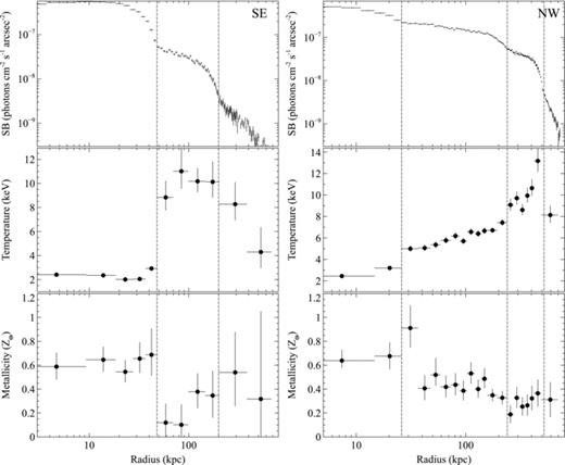
Surface brightness, temperature and metallicity profiles for the SE (left-hand panels) and NW (right-hand panels) sectors shown in Fig. 5. The surface brightness profiles cover the energy range 0.5–7 keV and edges, corresponding to cold fronts or shocks, are marked by the dashed lines. Note that the sectors were not selected to correspond to the shock edges (see Fig. 11).
The surface brightness edges corresponding to the shock fronts and the contact discontinuity ahead of the subcluster core are clearly visible in Fig. 6, but we also note two additional edges in the NW sector immediately behind the subcluster core at 26 kpc and at the end of the subcluster tail at 240 kpc. The surface brightness drop immediately behind the subcluster core is also accompanied by an increase in the gas temperature from 3.2 ± 0.1 to 5.0 ± 0.3 keV. Interestingly, the AGN and centre of the BCG are located almost exactly at the position of this surface brightness and temperature edge. The AGN was excluded from the spectral fits using a region of radius 2 arcsec and therefore did not contribute to the temperature increase at this location. It is more likely that this contact discontinuity has been created by the convergence of the surrounding ICM behind the dense subcluster core. The metallicity immediately behind the core appears consistent with the core value, although with large errors. The metallicity then decreases to  and is approximately constant through the subcluster tail. Metal-rich material that is ram pressure stripped from the subcluster core may build up in the region immediately behind the core where the flow of the ambient ICM converges.
The surface brightness edge at the end of the subcluster tail (at 240 kpc) is broad, covering ∼80 kpc in radius, and has a relatively shallow surface brightness gradient that does not appear to be characteristic of a contact discontinuity. The temperature gradient increases from 6.7 ± 0.2 to 9.1+0.6−0.5 keV across this region. However, there is likely to be a significant component of projected emission on this region which will increase the apparent temperature. Deprojection routines usually assume spherical symmetry which is not a good assumption for this region of Abell 2146 where the cluster emission is strongly elongated along the merger axis and the surface brightness gradient is relatively shallow. This surface brightness edge marks the region where 6–7 keV material from the end of the subcluster tail could be mixing with gas from the primary cluster.
Fig. 7 shows the surface brightness and temperature of the gas in the SW plume and a comparison no-plume sector on the other side of the subcluster tail (see Fig. 5). These two sectors were also each compared with two neighbouring sectors positioned on either side to the NW and SE. Fig. 7 (left-hand panels) shows the surface brightness enhancement of the plume over the surrounding sectors from ∼50 to 250 kpc. The electron pressure is possibly higher in the sector to the SE of the plume as the temperature is higher here but the errors are large; otherwise, the plume is in pressure equilibrium with the surroundings. There is no comparable surface brightness increase in the no-plume sector. The increase in temperature in the NW no-plume sector is probably due to the inclusion of a section of the upstream shock in the region analysed. The metallicity is approximately constant at  , similar to the ambient ICM, for both plume and no-plume sectors.
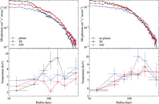
Surface brightness and temperature profiles for the plume and no-plume sectors shown in Fig. 5. The NW and SE profiles refer to additional, comparison sectors positioned on either side of the plume and no-plume sectors.
We suggest that the plume is likely to be the remnant of the primary cluster core which has been pushed forward and laterally by the impact of the subcluster core. There does not appear to be a symmetric structure extending from the merger axis to the NE, but this can be explained if the two clusters collided with a non-zero impact parameter (see e.g. Roettiger, Stone & Mushotzky 1998; Ricker & Sarazin 2001; Poole et al. 2006). Simulations of off-axis mergers indicate that if the subcluster passed to the north of the primary cluster centre, at a distance of the order of the core size, material from the primary core would be ejected perpendicular to the merger axis in the SW direction, as observed in Abell 2146. A strongly off-axis collision, comparable to the lateral extent of the shock fronts, seems unlikely, however, as the two shock fronts are both close to symmetric about the merger axis and the primary cluster core has been strongly disrupted by the merger. Detailed simulations of the merger in Abell 2146 will be needed to improve these rough limits.
3 THE SHOCK FRONTS
3.1 Surface brightness profiles
Fig. 8 shows the sectors selected for the analysis of the bow and upstream shock fronts. The sectors were positioned according to the centre of curvature of the edge and cover an angular range where the shock front is well defined. These sectors were divided into radial bins initially of 1 arcsec width but this was increased to 1.5, 2.5 and 5 arcsec at larger radii to ensure a minimum of 50 source counts in each bin. Point sources were excluded from the analysis and the background was subtracted using the normalized blank sky background data sets detailed in Section 2.1. To maximize the S/N, the surface brightness profiles were restricted to the energy range 0.5–4.0 keV and we used only the Chandra observations taken with ACIS-I, which have a lower background than ACIS-S. Fig. 9 shows the final background-subtracted X-ray surface brightness profiles for the two shock fronts. We fit the surface brightness edge associated with each shock with a model for a projected spherical density discontinuity, assuming that the edge is symmetric about the merger axis (e.g. Markevitch et al. 2000, 2002; Owers et al. 2009). The model radial gas density profile consists of a power law on either side of an abrupt density jump where the free parameters are the slopes and normalizations of the power laws and the radial position of the density jump. The corresponding emission measure profile was projected on to the sky and fitted to the observed surface brightness profile over a radial range selected to exclude unrelated core structures but extending to large radii for correct projection.

Unsharp-masked image (as in Fig. 2, upper right-hand panel) showing the sectors used to produce surface brightness profiles for the shock fronts. The sectors were centred on the centre of curvature for each shock front.
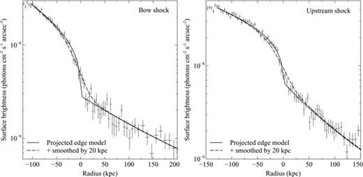
Left-hand panel: background-subtracted surface brightness profile across the bow shock in the energy band 0.5–4.0 keV overlaid with the best fitting projected density discontinuity model with no smoothing (solid lines) and with 20-kpc smoothing, corresponding to the mean free path λin → out (dashed lines). Right-hand panel: same as the left-hand panel but for the upstream shock.
At the bow shock, the density drops by a factor ρ2/ρ1= 2.5 ± 0.2 which gives a Mach number M= 2.3 ± 0.2. For the upstream shock, the density decreases by ρ2/ρ1= 1.9 ± 0.2 producing M= 1.6 ± 0.1.
Even in the raw counts image shown in Fig. 1 it is clear that the upstream shock in Abell 2146 has a very narrow edge separating the pre- and post-shock gas. We estimated the width of the shocks by smoothing the best-fitting density discontinuity model with Gaussian functions of varying widths, σ, and fitting the smoothed models to the surface brightness profile across the shock front. For the upstream shock, the best-fitting model with zero width has χ2= 98.4 for 85 degrees of freedom. This is reduced to χ2= 88.9 for 84 degrees of freedom for a smoothed model with a width  (95 per cent errors). Fig. 9 shows that the bow shock is broader than the upstream shock with a best-fitting width of 12+6−5 kpc (95 per cent errors).
The shock widths can be compared with the Coulomb mean free path of the electrons and protons on both sides of the shock front. Following Vikhlinin et al. (2001a), we estimate the mean free path for particles crossing from the post-shock gas into the pre-shock gas, λin → out, which is the main source of diffusion across the edge. For the bow shock, the mean free path λin → out= 21 ± 3 kpc and for the upstream shock it is 23 ± 5 kpc. If Coulomb diffusion is not suppressed across the shock edge, we expect the shock to have a width of several times the mean free path. The upstream shock is significantly narrower than the estimated mean free path, which suggests there is a significant suppression of transport processes across this edge consistent with a collisionless shock.
The bow shock appears broader; however, the measured width of the shock fronts can be affected by any deformations in the front shape, which smear the edge in projection. It is therefore difficult to determine if the bow shock front is intrinsically wider.
The estimated width of the Bullet cluster bow shock is ∼35 kpc, although Markevitch (2006) find this is only marginally preferred over a zero width shock. It is, however, surprising that the upstream shock front should be the narrowest when it is propagating through the remaining infall from the subcluster’s passage.
Fig. 10 shows the variation in the surface brightness profile of each shock front with position angle. The bow shock appears to be slightly stronger in the central sector but the lower number of counts in this sector, particularly in the pre-shock region, increases the error on the density jump value and this is therefore not a significant result. Both the bow and the upstream shock fronts appear to be consistently narrow across their respective lengths of ∼500 and ∼440 kpc.
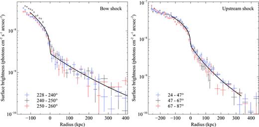
Background-subtracted surface brightness profiles of the bow shock (left-hand panel) and upstream shock (right-hand panel) each divided into three sectors showing the variation in the shock width and strength with position angle. The best-fitting projected discontinuity models generated for the full width of the shock fronts in Section 3.1 are shown overlaid.
3.2 Spectral analysis of the shock fronts
The temperature jump across the shock front can be used to derive an independent measure of the Mach number and to calculate the shock velocity to determine the time since core passage of the subcluster. Fig. 11 shows the projected temperature, projected metallicity and deprojected electron density profiles for the bow shock and upstream shock sectors (see Fig. 8). These radial profiles have the same radius of curvature as each of the two shock fronts and therefore clearly show the temperature and density decreases across the shock edges. We calculated the deprojected temperature profile across each shock front using projct in xspec. Deprojection routines, such as projct, generally assume that the cluster is spherically symmetric, which is a reasonable assumption for a relaxed cluster but can be problematic for major mergers. However, for the sectors across the shock fronts, the cluster appears approximately circular on the sky and the sharp increase in surface brightness across the edge reduces the impact of projected emission. The large size of the radial bins used to measure the temperature values is likely to be a more significant source of error in determining the temperature jump across each shock.
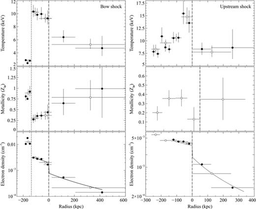
Radial profiles through the bow (left-hand panels) and upstream (right-hand panels) shock sectors (shown in Fig. 8) showing the projected electron temperature (upper panels), projected metallicity (middle panels) and deprojected electron density (lower panels). There are two sets of points showing a finer (filled points) and a broader (open points) radial binning. The electron density model (solid line) shown corresponds to the best fit to the surface brightness profile across each shock (Section 3.1). The vertical long-dashed line shows the location of each shock front and the vertical short-dashed line shows the position of the cold front on the leading edge of the subcluster core.
We find that the deprojected temperature decreases by a factor of T2/T1= 1.8 ± 0.3 at the bow shock and T2/T1=2.1+0.4−0.3 at the upstream shock. The Rankine–Hugoniot shock jump conditions directly relate the temperature jump to the density jump. We can therefore calculate the expected density jump and Mach number of each shock (equation 1) from the observed temperature jump as an independent verification (Landau & Lifshitz 1959). We calculate a Mach number M=1.8+0.3−0.2 for the bow shock and M= 2.0 ± 0.3 for the upstream shock. The Mach number for both shock fronts is therefore consistent within the errors for the calculations using both the temperature and the density jumps. The temperature jump provides a less accurate measure of the Mach number as the errors are greater than for the density and larger radial bins must be used to measure the temperature so we cannot resolve the jump across the shock accurately.
By using the bow shock speed and estimating the distance between the subcluster core and the primary cluster centre, we calculate the time since the subcluster passed through the primary cluster core. The shock speed, v, is calculated by multiplying the shock Mach number and the sound speed in the pre-shock gas cs= (γkBT1/mHμ)1/2, where T1 is the pre-shock gas temperature and μ= 0.6 is the mean molecular weight in the ICM. For the bow shock in Abell 2146, we use the Mach number calculated from the density jump M= 2.3 ± 0.2 and calculate the pre-shock sound speed to be cs=1170+100−70 km s−1, giving a shock velocity v=2700+400−300 km s−1 . However, even in the new, deep Chandra observations, it is not possible to conclusively identify an X-ray peak associated with the primary cluster core (Fig. 4, upper left-hand panel). Simulations suggest that if the primary cluster halo has a low concentration, the core will not survive a major collision and the X-ray peak will be destroyed (e.g. Mastropietro & Burkert 2008). We have therefore assumed that the collision between the two cluster cores occurred at a peak in the pressure map between the subcluster tail end and the upstream shock (Fig. 4, left-hand panels). The distance between the subcluster core and the estimated location of the core collision site is then ∼350 kpc and the time since core passage is therefore ∼0.1–0.2 Gyr. This is only a rough estimate of the time-scale as the subcluster velocity is likely to be significantly lower than the shock velocity (Springel & Farrar 2007) and the location of the collision site may be closer to the subcluster tail and the plume. However, it is clear from the detection of the shock fronts and the SW plume structure that this merger is observed recently after core collision.
Fig. 11 (left-hand panels) also shows that there is a sharp change in the gas properties across the cold front at the leading edge of the subcluster cool core. The temperature increases by a factor of 3.7+0.3−0.2 (discussed further in Section 4.2), whilst the metallicity drops from  inside the subcluster core to
  in the post-shock gas. The sharp metallicity drop clearly demonstrates the different origins of the ICM on either side of the contact discontinuity. The high-metallicity core from the subcluster is travelling through the ICM in the outskirts of the primary cluster, which has a much lower metallicity. In comparison, the upstream shock sector (Fig. 11, right-hand panels) has an approximately constant metallicity of 0.3–
 , as it consists predominantly of primary cluster gas. There may be more metal-enriched ram pressure stripped material from the subcluster in this sector; however, the material that was stripped from the core earlier is likely to have a lower metallicity than the current peak and the subcluster tail shows no evidence of a strong metallicity gradient (Fig. 4).
3.3 The establishment of electron–ion equilibrium
Cluster merger shock fronts present a unique opportunity to investigate the electron–ion equilibration time in the magnetized ICM by mapping the post-shock electron temperature. The Rankine–Hugoniot shock jump conditions can be used to calculate the post-shock temperature for the ICM electrons and ions once they reach equilibrium after the passage of the shock (e.g. Landau & Lifshitz 1959). However, the fraction of a shock’s kinetic energy that is initially transferred to the thermal and cosmic-ray populations of the electrons and ions remains an open question.
However, shocks in a magnetized plasma, such as the ICM, are likely to be collisionless. Observations of the solar wind shocks found that the electron and ion temperature jumps occur in a shock layer several orders of magnitude thinner than the mean free path (e.g. Ness, Scearce & Seek 1964; Montgomery, Asbridge & Bame 1970; Hull et al. 2001). The coupling of particles to electric and magnetic fields produces interactions which have dissipation scalelengths much shorter than the ordinary collision mean free path. The plasma waves producing these interactions and instabilities affect ions and electrons differently due to the large difference in mass (for a review, see e.g. Tidman & Krall 1971; Friedman et al. 1971). We might therefore expect to find an electron heating rate shorter than the Coulomb collisional time-scale behind a cluster merger shock.
Measurements of the post-shock temperatures in supernova remnants (e.g. Rakowski 2005; Raymond & Korreck 2005; Ghavamian, Laming & Rakowski 2007) and heliospheric shocks (e.g. Schwartz et al. 1988; Russell 2005) show that in most cases the electrons are heated less than the protons, Te/Ti < 1, in regions close to the shock front. However, these measurements cannot determine the time-scale of subsequent equilibration, teq(e, p), as this corresponds to a linear scale of several au for planetary bow shocks and is comparable to the age of the remnant for supernova shocks. For cluster merger shock fronts, the equilibration time-scale corresponds to a distance of hundreds of kpc, so while clusters are too distant for us to resolve the shock layer, we can study the subsequent equilibration of the ICM constituents.
The bow shock in the Bullet cluster provided the first measurement of the electron–ion equilibration time-scale in the ICM. Markevitch (2006) compared the observed electron temperature profile across the shock front with two models for equilibration. The instant equilibration model predicts that the electrons are strongly heated at the shock front and the electron temperature rapidly increases to the post-shock temperature, similar to the ion temperature. The collisional model predicts an adiabatic compression of the electron population at the shock and a subsequent slower equilibration with the ions on a time-scale determined by Coulomb collisions. The observed temperature profile for the Bullet cluster supported instant equilibration, indicating that electrons were rapidly heated at the shock front on a time-scale faster than Coulomb collisions. However, the post-shock temperature in the Bullet cluster is very high (∼20–40 keV) compared to the Chandra energy band and therefore difficult to constrain.
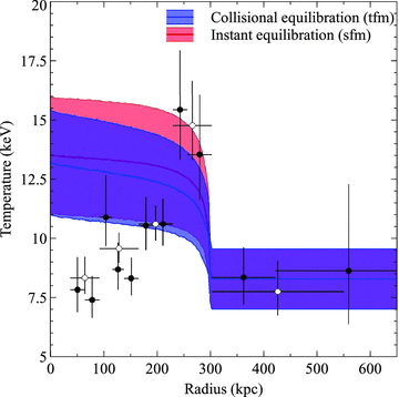
Although the post-shock temperatures in Abell 2146 are lower than the Bullet cluster, the shock Mach numbers are also lower, which reduces the separation between the collisional and instant equilibration models. Figs 12 and 13 show the observed and model projected electron temperature profiles behind the bow shock and upstream shock, respectively. The observed profiles were generated using single-temperature-model fits to spectra extracted from two different sets of radial bins. The narrower radial bins were selected to contain a minimum of 2000 counts and the broader bins have a minimum of 4000 counts. The post-shock radial bin closest to the shock boundary was positioned to overlap the fainter pre-shock gas and ensure minimal contamination of the neighbouring pre-shock gas radial bin.
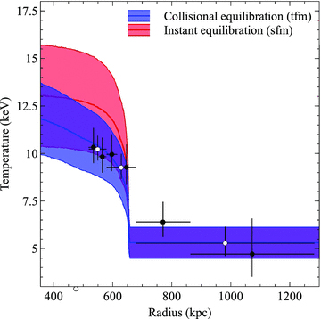
The re-establishment of electron–ion equilibrium behind the bow shock. The projected electron temperature profile is overlaid with model predictions (with 1σ error bands) for instant equilibration (red) and adiabatic compression followed by collisional equilibration (blue). The open and filled data points show narrower and broader binning of the temperature profile.
The re-establishment of electron–ion equilibrium behind the upstream shock. The projected electron temperature profile is overlaid with model predictions (with 1σ error bands) for instant equilibration (red) and adiabatic compression followed by collisional equilibration (blue). The open and filled data points show narrower and broader binning of the temperature profile.
The models were generated by using the observed pre-shock electron temperature and the density jumps in the Rankine–Hugoniot shock jump conditions to predict the post-shock gas temperature. For the instant equilibration model (a single-fluid model), the electron temperature and the ion temperature jump at the shock front to the post-shock gas temperature predicted by the shock jump conditions. This temperature model was then projected along the line of sight, using the best-fitting surface brightness model determined for each shock front in Section 3.1, to produce the final projected temperature model. The projection smoothes the sharp jump in temperature at the shock front. Although the projection assumes a constant pre-shock temperature, the steep decline in the surface brightness across and ahead of each shock front (Fig. 9) meant the effect of any cooler gas beyond the observed temperature points is negligible.
 , upstream shock
  ), we determine the distance behind the shock where equilibration is reached. Electrons at this position were heated by the shock teq yr ago. By integrating equation (4), and using equations (2) and (5), the electron temperature as a function of distance behind the shock was determined analytically (see e.g. Fox & Loeb 1997; Ettori & Fabian 1998). This collisional model was then also projected along the line of sight to produce the final model for comparison with the observed projected electron temperature.
The instant and collisional models were projected by determining the model electron temperature in small volumes, dV, along the line of sight for a particular annulus and calculating the corresponding emission measure using the best-fitting density discontinuity model (Section 3.1). For each annulus, the emission measures for dV with similar temperatures were summed together using a set temperature binning with fine resolution (∼0.1 keV). To determine the projected temperature in this annulus, we produced fake spectra in xspec using multicomponent MEKAL models with the temperature of each component set to the mid-point of each temperature bin and the normalization set to the corresponding summed emission measure. The metallicity was fixed to  and responses for the appropriate detector region were used. The MEKAL model components were also combined with a PHABS absorption component set to the Galactic column density. These fake spectra were then fitted with single absorbed MEKAL models, with fixed metallicity and column density, to determine the final model projected temperature.
The main sources of error for these models were the measurement of the pre-shock temperature and, to a lesser extent, the density jump and pre-shock electron density. We used a Monte Carlo technique to determine the uncertainties in the model-projected temperature profiles. We repeated the model calculation and projection 1000 times, each time using new values of the pre-shock temperature, density jump and pre-shock density based on Gaussian distributions. The output models are the median of this process and the 1σ errors are calculated from the 15.85 and 84.15 percentile spectra.
Fig. 12 shows the observed and model projected electron temperature profiles across the bow shock. The observed temperature profile is cut off ∼150 kpc behind the bow shock front where the temperature drops in the subcluster core. Unfortunately, owing to the large uncertainty on the pre-shock count rate in the earlier 45 ks observation, there were fewer pre-shock counts in the new 400 ks observation than anticipated. The lower number of counts produced a greater than expected error on the crucial pre-shock temperature, which is the main source of uncertainty for the models, and therefore it is not possible to conclusively exclude either model. However, the observed post-shock electron temperatures for the bow shock appear lower than predicted by the instant equilibration model and favour the collisional equilibration model. We therefore conclude that collisional equilibration cannot be ruled out for cluster merger shocks.
The pre-shock temperature could potentially be higher than the conservative estimate of 5.3+0.9−0.7 keV used in this analysis. The temperature bin closest to the bow shock front has a slightly higher temperature of 6.4+1.1−0.8 keV. This increase in temperature could be due to contamination from the higher temperature and density post-shock regions. However, the neighbouring post-shock temperature bin was positioned to significantly overlap the pre-shock region by 20 kpc (6 arcsec) and minimize this effect. It is therefore more likely that there is a gradient in the pre-shock gas temperature which would increase the post-shock temperature of both models and strengthen our conclusion that collisional equilibration is possible for cluster merger shocks.
Measurement of the equilibration time-scale was more difficult for the upstream shock as the Mach number was lower, reducing the separation between the instant and collisional models. In addition, the post-shock electron temperatures are ∼5 keV higher compared to the bow shock, which increased the uncertainty on the values. Fig. 13 shows that the electron temperature increases rapidly in the post-shock region to 15+2−1 keV and then drops to ∼10 keV approximately 100 kpc behind the shock front. Although the errors are larger, the electrons behind the upstream shock appear to equilibrate faster than those at the bow shock. However, the upstream shock is also propagating through the primary cluster outskirts, which have been disturbed by the subcluster’s passage. There is likely to be significant substructure and additional shock heating in the region of the upstream shock front. Ram pressure stripped material from the subcluster tail is likely to be the cause of the rapid decline in temperature ∼70 kpc behind the shock. We therefore place less weight on the conclusions on equilibration behind the upstream shock as the situation here is more complex and the errors on the electron temperature are greater.
3.4 Non-equilibrium ionization
In the previous section, we have shown that the post-shock ICM significantly deviates from thermal equipartition between electrons and ions, but our analysis has so far assumed that the ICM is in ionization equilibrium. However, while the temperature of the ICM increases rapidly in the shock layer, the ionization state of the ions still reflects the pre-shock temperature and the ICM will be underionized compared to the equilibrium case. The ionization balance will be recovered by collisions on a time-scale of ∼107 yr for an electron density ∼10−3 cm−3 but until this is achieved there will be more ionizations than recombinations. Simulations of the outer regions of clusters and of merging systems have considered the effects of non-equilibrium ionization, in particular the effect on the intensity ratios of the Fe Kα lines (e.g. Yoshikawa & Sasaki 2006; Akahori & Yoshikawa 2010, 2012; Wong, Sarazin & Ji 2011). We have therefore considered whether non-equilibrium ionization will produce an observable effect in the post-shock ICM of Abell 2146.
For a temperature of ∼9 keV (108 K) behind the bow shock, the typical density-weighted time-scale for the ions to approach ionization equilibrium is  for Fe and significantly shorter for other important ions in the ICM (e.g. Smith & Hughes 2010). Using the post-shock electron density,
  , and the velocity of the shock in the post-shock gas (Section 3.3), we estimate that the Fe ions reach equilibrium ionization ∼50 kpc behind the bow shock. Therefore, only the first narrow radial bin behind the bow shock (and also for the upstream shock) could be affected by non-equilibrium effects.
We fit each of these radial bins, immediately behind each shock front, with an absorbed non-equilibrium ionization nei spectral model in xspec (e.g. Hamilton, Sarazin & Chevalier 1983; Borkowski, Lyerly & Reynolds 2001). The nei model indicated a density-weighted ionization time-scale of  behind each shock front, suggesting that there was no measurable signature of non-equilibrium ionization in Abell 2146. This is a difficult measurement, given the low spectral resolution at high energies, covering the Fe xxv Kα and Fe xxvi Kα lines (Akahori & Yoshikawa 2010, 2012), and the low photon count rates at the shock front, necessitating large radial bins relative to the ionization equilibration time-scale.
4 DISRUPTION OF THE SUBCLUSTER CORE
Fig. 14 shows the detailed structure in the subcluster core and ram pressure stripped tail. The front edge of the subcluster core appears roughly spherical, but the sides are strongly sheared by the surrounding shocked gas. The southern edge of the subcluster core appears to be narrow with no sign of disruption and stripping which affect the eastern and northern edges (e.g. Fig. 2). The temperature gradients on the SW and NE sides of the subcluster core are very different. There is clearly a more graduated increase in temperature along the NE edge where the core is breaking up.
Left-hand panel: projected pseudo-pressure map of the subcluster tail with S/N ≥ 32 in each bin (in units of keV cm−5/2 arcsec−2). Right-hand panel: projected temperature map (in units of keV) of the same region with S/N ≥ 32. The excluded central AGN is visible as a small white circle. The circles mark a region where the temperature gradient through the subcluster tail reverses from 6–6.5 keV (dashed) to 5 keV gas (solid).
Fig. 15 shows that the filament of gas running along the southern edge of the core, and apparently ending at the AGN, contains the coldest gas in the cluster. Using a single-temperature spectral model (Section 2.3), we determined that the X-ray gas temperature drops to 1.48+0.09−0.08 keV in this filament. This cool X-ray gas filament is also detected as a narrow, coherent filament in Hα and [N ii] observations (Canning et al. 2011). We fitted the spectrum from this region (shown in Fig. 15) with a multitemperature model to determine if there is a significant amount of multiphase gas detectable in the X-ray. Following Sanders et al. (2004), we used multiple absorbed mekal components with temperatures fixed at 0.5, 1, 2 and 4 keV, common metallicities and free normalizations. We tested an additional 8 keV component but found that the best-fitting normalization was consistent with zero. The majority of the gas in the filament is at around 2 keV, but we detect significant amounts of cooler gas. The fraction of the emission measure of gas at 1 keV, with respect to the total emission measure, is 15–20 per cent and at 0.5 keV is 5–10 per cent. Both of these lower temperature components are detected at above 3σ. The best-fitting metallicity for this multitemperature model is  . It is therefore likely that the low metallicity observed in the subcluster core in Figs 4 and 6 is a bias caused by the use of only a single-temperature model (Buote & Canizares 1994; Buote 2000).
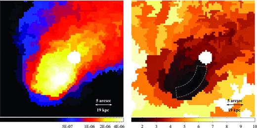
Left-hand panel: projected emission measure per unit area map of the subcluster core with S/N ≥ 15 in each bin (in units of cm−5 arcsec−2, see Fig. 4). Right-hand panel: projected temperature map (in units of keV) of the same region with S/N ≥ 22. The white dashed region marks the cold gas filament. The excluded central AGN is visible as a small white filled circle in both images.
Using an absorbed mekal+mkcflow model, with the lower temperature of the mkcflow component (Mushotzky & Szymkowiak 1988) fixed to 0.1 keV, the upper temperature component tied to the temperature of the MEKAL model and the metallicities tied together, we determine an upper limit on the mass deposition rate for the filament region of  , which is cooling out of the X-ray band (see e.g. McNamara et al. 2006; Rafferty et al. 2006). The upper limit on the mass deposition rate for the whole of the subcluster core is
  ; therefore, the vast majority of the cooling in the subcluster core is likely occurring in this filament. This is significantly less than the star formation rate (SFR) of
  determined from Spitzer observations of the BCG by O’Dea et al. (2008). However, the IR emission was not corrected for an AGN contribution, which is likely to dominate (Canning et al. 2011), and therefore this SFR is an upper limit and the true rate is likely to be much lower.
4.1 Stripping of the NE edge
Fig. 15 shows the stripping of cool material from the eastern edge of the subcluster cool core. Cool gas is being pulled off the eastern edge of the core into a 12 arcsec (45-kpc) filament which has a steadily increasing temperature from 1.9 ± 0.1 to 3.1+0.5−0.4 keV along its length, although this could be affected by hotter material seen in projection. There are several cooler blobs of gas to the north and NW of the AGN, suggesting this material then breaks off and may be directed towards the west into the subcluster’s wake. Warmer 3–4 keV gas appears to be filling underneath the cool, stripped filament. The coolest gas in the subcluster core is towards the leading southern edge of the core.
Simulations of ram pressure stripping of a cool core during a cluster merger show strong shearing of the contact discontinuity and the formation of a strong vortex inside the core, which transports material inside the core to the leading edge and then back along the surface travelling with the surrounding flow (e.g. Murray et al. 1993; Balsara, Livio & O’Dea 1994; Heinz et al. 2003). The cooler blobs of gas stripped off the eastern edge trace the flow of material around the subcluster core and show the flow converges behind the core, at the approximate position of the AGN (see Section 2.3.2).
In Section 2.3.2, we suggest the subcluster is likely to have passed to the north of the primary cluster core, colliding with a small but non-zero impact parameter. This trajectory will produce a more curved orbit for the subcluster core, trending from a SE direction to southern, compared to the case of the head-on collision. The southern edge is now the leading edge of the subcluster core and there is likely to be a greater shearing effect on the eastern edge due to the curved trajectory.

 . For
. For  and
and  , we find that the condition for ram pressure stripping is only approximately met along the eastern edge of the core although the pressure does not steeply increase here as observed inside the southern edge (Fig. 16, lower right-hand panel). Therefore, it is likely that the removal of material along this edge is also facilitated by developing Kelvin–Helmholtz instabilities (Nulsen 1982; Inogamov 1999). However, without a more effective estimate of the velocity of the ambient ICM around the subcluster core it is difficult to calculate the time-scale of the developing instabilities and determine whether the subcluster core will be subsequently destroyed (e.g. Vikhlinin et al. 2001b; Heinz et al. 2003).
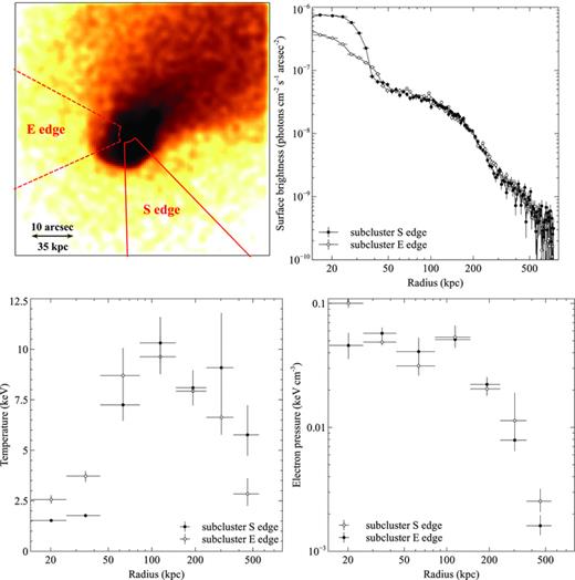
Surface brightness (upper right-hand panel), projected temperature (lower left-hand panel) and electron pressure profiles (lower right-hand panel) for two sectors across the southern (filled circles, 270°–315°) and eastern (open circles, 150°–205°) edges of the subcluster core. An image showing the sectors used is also included (upper left-hand panel). The electron pressure profiles were produced by multiplying the deprojected electron density and the deprojected electron temperature profiles.
4.2 Width of the subcluster southern edge
In comparison, the SW edge of the subcluster core and tail appears to be narrow and stable over a distance of 150 kpc (e.g. Fig. 2). Fig. 16 (upper right-hand panel) shows that the surface brightness drops by close to an order of magnitude at a distance of only ∼15 kpc across the narrowest point of the southern edge. The eastern edge of the subcluster core shows a much more gradual decline in surface brightness with no obvious sharp edge corresponding to a density jump. The deprojected temperature, determined using projct in xspec, increases rapidly across the narrow southern edge of the subcluster core by a factor of 3.4+0.9−0.6. The gas in the subcluster core is multiphase and the temperature jump for the cooler 0.5 keV component could be higher by a factor of a few. Unless suppressed by at least an order of magnitude, thermal conductivity in unmagnetized cluster gas should rapidly evaporate the cool subcluster on a time-scale of only ∼107 yr (e.g. Ettori & Fabian 2000; Markevitch et al. 2003; Asai, Fukuda & Matsumoto 2004).
To determine the density jump across the subcluster southern edge, we fit the surface brightness profile with the model for a projected spherical density discontinuity discussed in Section 3.1. A surface brightness model for the outer cluster emission, a β model (Cavaliere & Fusco-Femiano 1976) plus a Gaussian component to account for the blurred bow shock edge, was added to the projected discontinuity model to ensure the projected emission was accounted for. Fig. 17 shows the best-fitting model for the surface brightness across the southern edge, assuming a discontinuous jump in the gas density, which produced a best-fitting density jump of 2.6 ± 0.2. We also smoothed the best-fitting model by convolving the density jump with a Gaussian function to determine if a non-zero width produced a better fit to the surface brightness edge. A model with σ= 0 provided the lowest χ2 and we calculated a 95 per cent upper limit on the cold front edge width of σ= 2 kpc.
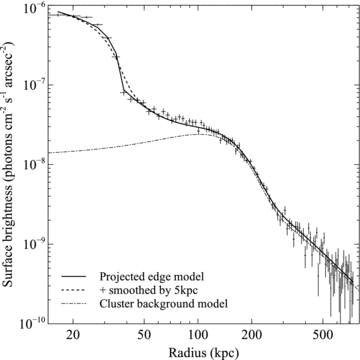
Surface brightness profile for the southern edge of the subcluster core with the best-fitting projected discontinuity model shown overlaid (solid line). The dashed line corresponds to the best-fitting projected discontinuity model smeared with a Gaussian of width σ= 5 kpc and the dot–dashed line shows the model for the outer cluster emission.
This upper limit on the width can be compared with the Coulomb mean free path of the electrons and protons on both sides of the cold front. As in Section 3.1, we estimate the mean free path for particles crossing from inside the subcluster core to the outside, λin → out= 0.5–1 kpc, which is the main source of diffusion across the edge. If Coulomb diffusion is not suppressed by any mechanism, then the southern edge should have a width of at least several times λin → out. Therefore, it is likely that transport processes are highly suppressed here. As discussed in the introduction, the gas motion around the subcluster core is likely to produce a preferentially tangential magnetic field and strongly restrict heat flux and diffusion across the front (e.g. Narayan & Medvedev 2001; Vikhlinin et al. 2001b; Asai, Fukuda & Matsumoto 2004, 2005, 2007; Lyutikov 2006; Xiang et al. 2007; Dursi & Pfrommer 2008; see also Churazov & Inogamov 2004).
4.3 Structure in the subcluster tail
The NE and SW sides of the subcluster tail appear strikingly different in this deeper Chandra observation. Even in the raw counts image (Fig. 1), the SW side of the tail exhibits a sharp, coherent edge that stretches ∼150 kpc in length. Fig. 2 (lower left-hand panel) indicates that there may be a second fainter edge, 100 kpc in length, outside the main edge. It is unclear whether these are different or related structures as the subcluster tail is clearly three dimensional and structures are seen in projection. The narrow SW edge of the subcluster tail appears similar to the sharp, straight edges of the subcluster bullet in the Bullet cluster which appear unaffected by turbulence (Markevitch 2006; Markevitch & Vikhlinin 2007). Turbulence may be suppressed along the SW edge of the core by a continuation of the magnetic layer that strongly restricts conduction across the leading edge of the cool core (Section 4.2; e.g. Lyutikov 2006; Xiang et al. 2007; Dursi & Pfrommer 2008).
In comparison, the NW edge is broad (∼few × 10 kpc across), and poorly defined as it is disrupted by the shearing flow of the ambient ICM. Small-scale instabilities are expected to grow rapidly on time-scales much shorter than the cluster passage time and widen the interface. If magnetic draping is responsible for the stability of the SW edge of the subcluster core and tail, then it is initially surprising that the eastern edge of the core is not similarly stabilized. However, as discussed in Section 2.3.2, the orbit of the subcluster core is likely to be curved to the south, which will increase the relative velocity of the ambient ICM along the NE edge of the core and reduce it along the SW edge. The ambient gas motion is responsible for the accumulation, stretching and ordering of the magnetic fields along the subcluster interface and an alteration in the subcluster trajectory could also affect the build-up of this magnetic draping layer. There is no significant variation in the thermal pressure along either side of the subcluster core (Fig. 14, left-hand panel), but there could be a significant variation in the flow velocity of the ambient ICM caused by the subcluster trajectory, which is affecting the stability of the eastern edge.
Fig. 14 shows the variation in the ICM pressure and temperature across the subcluster tail. The thermal pressure peaks in the dense, cool subcluster core but is also high behind the AGN where the flow of the ambient ICM converges behind the core. Although there is some fluctuation in pressure through the subcluster tail, and the eastern edge of the core appears to be breaking up, there are no significant structures consistent with large-scale hydrodynamic instabilities (e.g. Abell 3667, Mazzotta, Fusco-Femiano & Vikhlinin 2002). The cool blobs of gas breaking off from the eastern edge of the cool core (Fig. 15) appear to thermalize rapidly with the surrounding hot ICM and there is a steadily increasing temperature gradient through the subcluster tail. There is some significant variation in temperature gradient along the northern edge of the subcluster tail (Fig. 14) where hotter 6–6.5 keV gas appears to be impacting a region of cooler 5 keV material. However, it is not clear if this relatively cool region has been stripped off the subcluster core and become isolated from the ∼8 keV ambient ICM or if it has a similar origin to the SW plume and is a remnant of the primary cluster core. Either way, this is likely to be a transient feature that will thermalize with the surrounding ICM.
5 SUMMARY
The deep Chandra observations of Abell 2146 have revealed a host of new and complex substructure. We confirm the detection of both a bow shock with Mach number M= 2.3 ± 0.2 and the first known example of an upstream shock, which has a Mach number M= 1.6 ± 0.1. The bow shock, located ahead of the cool subcluster core, can now be traced to over ∼500 kpc in length and appears significantly broader than the upstream shock. We find that the observed post-shock electron temperature profile behind the bow shock is lower than predicted for instant shock heating of the electrons and appears consistent with the time-scale for Coulomb collisional equilibration with the ions. The equivalent measurement for the upstream shock appears to support the instant shock-heating model, similar to the result for the Bullet cluster. However, this measurement was more difficult for the upstream shock as the Mach number was lower, the uncertainty on the temperature values was greater and there is significant substructure generated by the passage of the subcluster core. We therefore place less weight on the result from the upstream shock.
In addition to the deviations from thermal equilibrium, we considered the possibility of non-equilibrium ionization in the region immediately behind each shock front. However, the relatively low spectral resolution, low photon count rates behind each shock front and large radial bins compared to the ionization equilibration time-scale make this a difficult measurement with the existing data.
Even in the raw counts image, the upstream shock appears remarkably narrow and well defined over ∼440 kpc in length. We calculate a best-fitting width for the shock of only 6+5−3 kpc (95 per cent errors), which is significantly narrower than the estimated mean free path and suggests that there is a significant suppression of Coulomb diffusion across the shock front. The bow shock appears broader with a best-fitting width of 12+6−5 kpc (95 per cent errors); however, the measured width of the shock fronts can be affected by deformations in the front shape which smear the edge in projection. Both the bow and upstream shock fronts appear to be consistently narrow across their measured lengths.
The deep Chandra observation has also revealed a cool, dense plume of material extending ∼170 kpc in length in a direction perpendicular to the merger axis. This plume is likely to be the remnant of the primary cluster core which has been pushed forward and laterally (SW) by the impact with the subcluster core. There does not appear to be a symmetric feature extending to the NE which suggests that the subcluster did not collide head-on with the primary cluster. If the subcluster passed to the northern side of the primary cluster, simulations suggest that disrupted material from the primary core would be mainly ejected in the direction of the observed plume. However, a large impact parameter seems unlikely, given the significant disruption of the primary core and the symmetry of the two shock fronts about the merger axis.
The surface brightness images of the subcluster core show a sharp, leading edge corresponding to an increase in the gas density by a factor of 2.6 ± 0.2 and temperature by a factor of at least 3.4+0.9−0.6. The gas in the core has a metallicity of  and is multiphase with significant temperature components at 2, 1 and 0.5 keV. We find an upper limit of
  on the mass deposition rate in the subcluster core and determine that ∼80 per cent of this cooling occurs in a bright filament. The leading edge of the subcluster core is particularly narrow with a 95 per cent upper limit on the width of only 2 kpc, compared to the mean free path of 0.5–1 kpc, so Coulomb diffusion is significantly suppressed here. We suggest that the motion of the subcluster core through the ambient ICM has produced a magnetic draping layer which strongly restricts conduction and diffusion across this edge.
The ram pressure stripped subcluster tail has interestingly different structure along its two sides, which are both being sheared by the surrounding medium. Cool gas is being stripped off the eastern edge of the core into a 45 kpc filament which has a steadily increasing temperature along its length. This material then breaks off the filament into small blobs of gas which are directed into the subcluster’s wake. The disrupted NE edge is broad at ∼few × 10 kpc across. In contrast, the SW edge is narrow and well defined over ∼150 kpc in length. The magnetic draping layer around the leading edge of the core could be stabilizing the SW edge against turbulent instabilities, but this appears to be less effective along the NE edge. For this non-zero impact parameter merger, the trajectory of the subcluster is likely to be curved to the south, which will increase the velocity of the ambient flow around the NE edge and could cause the observed gas stripping.
HRR and BRM acknowledge generous financial support from the Canadian Space Agency Space Science Enhancement Program. HRR also acknowledges support for this work provided by the National Aeronautics and Space Administration through Chandra Award Number 16617775 issued by the Chandra X-ray Observatory Center, which is operated by the Smithsonian Astrophysical Observatory for and on behalf of the National Aeronautics and Space Administration under contract NAS8-03060. ACF and LJK thank the Royal Society for support. REAC acknowledges funding from the STFC. SAB is supported in part by the Radcliffe Institute for Advanced Study at Harvard University. We thank the reviewer for helpful and constructive comments. We thank Poshak Gandhi and Sakurako Okamoto for help with the Subaru observations of Abell 2146. We thank Eugene Churazov, Roderick Johnstone and Julie Hlavacek-Larrondo for helpful discussions.
Footnotes
Note that equation (2) in Russell et al. (2010), relating the Mach number to the temperature jump, is applicable only for strong shocks. Given the large error on the temperature values in Russell et al. (2010), this had a negligible effect but as the temperature errors are much smaller for this deeper Chandra observation a similar assumption is not made here.
REFERENCES
