


Abstract
Broad absorption lines (BALs) in quasar spectra indicate high-velocity outflows that may be present in all quasars and could be an important contributor to feedback to their host galaxies. Variability studies of BALs help illuminate the structure, evolution and basic physical properties of the outflows. Here we present further results from an ongoing BAL monitoring campaign of a sample of 24 luminous quasars at redshifts 1.2 < z < 2.9. We directly compare the variabilities in the C ivλ1549 and Si ivλ1400 absorption to try to ascertain the cause(s) of the variability. We find that Si iv BALs are more likely to vary than C iv BALs. When looking at flow speeds >−20 000 km s−1, 47 per cent of quasars exhibited Si iv variability while 31 per cent exhibited C iv variability. Furthermore, ∼50 per cent of the variable Si iv regions did not have corresponding C iv variability at the same velocities, while nearly all occurrences of C iv variability had corresponding changes in Si iv. We do not find any correlation between the absolute change in strength in C iv and in Si iv, but the fractional change in strength tends to be greater in Si iv than in C iv. When both C iv and Si iv varied, those changes always occurred in the same sense (either getting weaker or stronger). We also include our full data set so far in this paper, which includes up to 10 epochs of data per quasar. The multi-epoch data show that the BAL changes were not generally monotonic across the full ∼5–8 yr time span of our observations, suggesting that the characteristic time-scale for significant line variations, and (perhaps) for structural changes in the outflows, is less than a few years. Coordinated variabilities between absorption regions at different velocities in individual quasars seem to favour changing ionization of the outflowing gas as the cause of the observed BAL variability. However, variability in limited portions of broad troughs fits naturally in a scenario where movements of individual clouds, or substructures in the flow, across our lines of sight cause the absorption to vary. The actual situation may be a complex mixture of changing ionization and cloud movements. Further discussion of the implications of variability, e.g. in terms of the size and location of the outflowing gas, will be presented in a forthcoming paper.
1 INTRODUCTION
High-velocity wind-like outflows are an important part of the quasar system and a potential contributor to feedback to the host galaxy. These outflows may play a crucial role in the accretion process in quasars and the growth of supermassive black holes (SMBHs), by allowing the accreting material to release angular momentum. Furthermore, quasar outflows may provide enough kinetic energy feedback to affect star formation in the quasar host galaxies, to aid in ‘unveiling’ dust-enshrouded quasars, and to help distribute metal-rich gas to the intergalactic medium (e.g. Di Matteo, Springel & Hernquist 2005; Moll et al. 2007).
Broad absorption lines (BALs) are the most prominent signatures of accretion disc outflows seen in quasar spectra. BALs are defined as absorption troughs with velocity widths >2000 km s−1 at depths >10 per cent below the continuum (Weymann et al. 1991), and they appear in the spectra of ∼10–15 per cent of quasars (Reichard et al. 2003; Trump et al. 2006; Knigge et al. 2008; Gibson et al. 2009). Since BALs are seen in just a fraction of quasar spectra, their presence could represent a phase in the evolution of a quasar and/or particular orientations where the outflow lies between us and the quasar emission sources.
The location and three-dimensional structure of quasar outflows are poorly understood. Sophisticated models predict these outflows as arising from a rotating accretion disc, with acceleration to high speeds by radiative and/or magneto-centrifugal forces (Murray et al. 1995; Proga, Stone & Kallman 2000; Proga & Kallman 2004; Everett 2005; Proga 2007). Improved observational constraints are necessary to test these models and to estimate mass-loss rates, kinetic energy yields and the role of quasar outflows in feedback to the surrounding environment.
One way to obtain constraints on quasar outflows is to study the variability in their absorption lines, which can provide information on the structure and dynamics of the outflowing gas. Two possible causes of this observed variability are movement of gas across our line of sight to the quasar and changes in ionization (Barlow 1993; Wise et al. 2004; Misawa et al. 2005; Lundgren et al. 2007; Gibson et al. 2008; Hamann et al. 2008). Variability on shorter time-scales can place constraints on the distance of the absorbing material from the central SMBH. Shorter variability time-scales indicate smaller distances, based on nominally shorter crossing times for moving clouds (Hamann et al. 2008; Capellupo et al. 2011) or the higher densities required for shorter recombination times (Hamann et al. 1997). Measurements of variability on longer (multi-year) time-scales provide insight into the homogeneity and stability of the outflowing gas. If no variability is detected on long time-scales, then this indicates a smooth flow with a persistent structure. Overall, results of variability studies provide information on the size, kinematics and internal make-up of substructures within the outflows. Furthermore, variability studies can address the evolution of these outflows as absorption lines have been observed to appear and disappear (Hamann et al. 2008; Leighly et al. 2009; Krongold, Binette & Hernández-Ibarra 2010; Rodríguez Hidalgo, Hamann & Hall 2011), or they can evolve from one type of outflow feature to another (e.g. from a mini-BAL to a BAL or vice versa; Gibson et al. 2010; Rodríguez Hidalgo et al., in preparation; also this work).
Most of the existing work on BAL variability has focused on variability in C ivλ1549 over two epochs (e.g. Barlow 1993; Lundgren et al. 2007; Gibson et al. 2008). Gibson et al. (2008) detected C iv BAL variability in 12 out of 13 BAL quasars (BALQSOs) (92 per cent) over multi-year time-scales. None of these studies found clear evidence for acceleration in the BALs. Gibson et al. (2010) report on variability on multi-month to multi-year rest-frame time-scales, using 3–4 epochs of data for nine BALQSOs and found that BALs generally do not vary monotonically over time. Their study also makes comparisons between variability in Si ivλ1400 absorption and variability in C iv, and their results include a correlation between fractional change in equivalent width (EW) in Si iv and C iv.
This work is the second paper in a series on BAL variability. The first paper, Capellupo et al. (2011, hereafter Paper 1), introduced our ongoing monitoring programme of a sample of 24 BALQSOs. We began with a sample of BALQSOs from Barlow (1993), which includes spectra of the C iv absorption region and, in most cases, coverage of the Si iv absorption region as well. We have re-observed these quasars to provide a longer time baseline over which to study variability, as well as to obtain multiple epochs of data per object. We currently have up to 10 epochs of data per quasar up to 2009 March, covering rest-frame time intervals (Δt) from 15 d to 8.2 yr.1
Paper 1 focused on a subset of the data from this monitoring programme to look for basic trends in the data between variability and other properties of the absorbers, as well as to directly compare short-term and long-term variability within the same sample of quasars. Paper 1 took a novel approach to studying BAL variability by introducing a measurement of BAL strength within portions of a trough, instead of using EW measurements. Paper 1 discusses variability in just two different time intervals: a short-term interval of 0.35–0.75 yr and a long-term interval of 3.8–7.7 yr. We found that 39 per cent (7/18) of the quasars varied in the short term, whereas 65 per cent (15/23) varied in the long-term data. The variability most often occurred in just portions of a BAL trough, which is similar to the findings of Gibson et al. (2008). We found that the incidence of variability was greater at higher velocities and in weaker portions of BAL troughs. Similarly, in Lundgren et al. (2007), the strongest occurrences of BAL variability occurred at velocities <−12 000 km s−1 and in features with smaller EWs. Overall, the results of Paper 1 are broadly consistent with previous work on BAL variability.
In this paper, we extend the analysis of Paper 1 by looking at variability in Si iv and comparing it to the variability results for C iv. Expanding our study to include Si iv absorption can help constrain theories on the cause(s) of BAL variability. C and Si have different abundances, if solar abundances are assumed, and they have different ionization properties (e.g. Hamann et al. 2008, 2011). By examining if C iv and Si iv have different variability properties, and how they differ, coupled with these differences in abundances and ionization properties, we can gain new insight into the cause(s) of BAL variability.
Our data set is uniquely suited to this study because we have coverage of the Si iv line for nearly our entire sample (22 out of 24 quasars). In addition to the larger sample size, we go beyond existing work by adopting a method of measuring the absorption strength in portions of BALs, instead of EW. EW measurements apply to an entire feature and are less sensitive to changes in small portions of troughs. Our method of measuring portions of troughs also allows more direct comparisons between the behaviour of C iv and Si iv variability.
We also include the entire data set so far to look at variability in C iv and Si iv over multiple epochs. This work contains up to 10 epochs of data per quasar, and including all of these epochs will provide better insight into the characteristics of BAL variability. Increasing the number of epochs provides new information on whether BALs change monotonically over time or whether they can vary and then return to an earlier state. In Paper 1, we reported that typically only portions of BALs varied. Multi-epoch data can tell us whether variability only occurs in those specific velocity intervals or if the velocity range over which variability occurs can change over time. We also highlight several individual interesting cases of variability that can further help us understand BAL outflows. Section 2 below reviews the quasar sample and analysis introduced in Paper 1, Section 3 describes our results, Section 4 summarizes the results so far from Paper 1 and the current work, and Section 5 discusses the results and their implications.
2 DATA AND ANALYSIS
2.1 Observations and quasar sample
In this work, we use the same sample of 24 BALQSOs introduced in Paper 1. This sample is based on the set of BALQSOs studied in Barlow (1993). The sample selection and general characteristics are described in Paper 1. These data were obtained from the Lick Observatory 3-m Shane Telescope, using the Kast spectrograph. Most of the spectra we use from that data set have a resolution of R≡λ/Δλ≈ 1300 (230 km s−1). For epochs where this resolution is not available, we use data taken at R≈ 600 (530 km s−1). BALs are defined to have a width of at least 2000 km s−1, so either of these resolutions is sufficient to measure the lines and study their variabilities. The wavelength coverage of each spectrum covers at least the Si iv through C iv emission lines, and most cover at least the Lyαλ1216 through C iv emission lines.
We have been re-observing 23 of the BALQSOs from Barlow (1993) at the MDM Observatory 2.4-m Hiltner telescope, using the CCDS spectrograph with a resolution of R≈ 1200 (250 km s−1). The observations used in this work were taken in 2007 January and February; 2008 January, April, and May; and 2009 January and March. We used the same spectrograph setup each time, varying only the wavelength range in order to observe each quasar at roughly the same rest wavelength range, from Lyα through C iv emission. One exception is 0946+3009, which has a redshift too low for the Si iv emission to appear in our spectra.
We supplement our data with spectra from the Sloan Digital Sky Survey (SDSS) Data Release 6 (Adelman-McCarthy et al. 2008) for eight of the quasars in our sample, for which the resolution is R≈ 2000 (150 km s−1). These spectra cover the observed wavelength range 3800–9200 Å, and we only include spectra that cover at least the Si iv through C iv emission.
Table 1 summarizes the full data set presented in this work, including the emission redshift, zem,2 and the ‘balnicity index’ (BI) for each object (as calculated in Paper 1). Any uncertainty in the redshift will not affect our comparisons between Si iv and C iv or any of our other results. The BI, defined by Weymann et al. (1991), is a measure of the strength of the BAL absorption and is calculated as an EW in units of velocity. It quantifies blueshifted C iv absorption between −25 000 and −3000 km s−1 that reaches at least 10 per cent below the continuum across a region at least 2000 km s−1 in width. The next four columns list the number of observations taken for each object at each observatory and then the total overall number of observations. The final column lists the range in Δt covered for each quasar.
Quasar data.
| Name | zem | BI | Lick 1988–92 | SDSS 2000–06 | MDM 2007–09 | Total | Δt (yr) |
| 0019+0107 | 2.130 | 2290 | 6 | 0 | 1 | 7 | 0.08–5.79 |
| 0043+0048 | 2.137 | 4330 | 2 | 2 | 1 | 5 | 0.35–6.13 |
| 0119+0310 | 2.090 | 6070 | 2 | 0 | 1 | 3 | 0.65–5.57 |
| 0146+0142 | 2.909 | 5780 | 2 | 0 | 2 | 4 | 0.52–5.15 |
| 0226−1024 | 2.256 | 7770 | 1 | 0 | 1 | 2 | 4.66 |
| 0302+1705 | 2.890 | 0 | 2 | 0 | 1 | 3 | 0.27–4.42 |
| 0842+3431 | 2.150 | 4430 | 6 | 1 | 3 | 10 | 0.06–5.87 |
| 0846+1540 | 2.928 | 0 | 5 | 0 | 3 | 8 | 0.04–4.93 |
| 0903+1734 | 2.771 | 10700 | 2 | 1 | 4 | 7 | 0.04–5.29 |
| 0932+5006 | 1.926 | 7920 | 4 | 1 | 4 | 9 | 0.05–6.98 |
| 0946+3009 | 1.221 | 5550 | 2 | 0 | 3 | 5 | 0.11–8.16 |
| 0957−0535 | 1.810 | 2670 | 2 | 0 | 2 | 4 | 0.11–6.21 |
| 1011+0906 | 2.268 | 6100 | 4 | 0 | 3 | 7 | 0.10–5.94 |
| 1232+1325 | 2.364 | 11000 | 1 | 0 | 2 | 3 | 0.35–5.93 |
| 1246−0542 | 2.236 | 4810 | 2 | 0 | 2 | 4 | 0.40–5.90 |
| 1303+3048 | 1.770 | 1390 | 1 | 0 | 4 | 5 | 0.05–6.10 |
| 1309−0536 | 2.224 | 4690 | 2 | 0 | 2 | 4 | 0.68–6.19 |
| 1331−0108 | 1.876 | 10400 | 2 | 1 | 2 | 5 | 0.42–5.97 |
| 1336+1335 | 2.445 | 7120 | 1 | 0 | 3 | 4 | 0.07–5.79 |
| 1413+1143 | 2.558 | 6810 | 2 | 1 | 2 | 5 | 0.26–5.61 |
| 1423+5000 | 2.252 | 3060 | 2 | 1 | 2 | 5 | 0.39–5.87 |
| 1435+5005 | 1.587 | 11500 | 2 | 0 | 2 | 4 | 0.34–7.72 |
| 1524+5147 | 2.883 | 1810 | 3 | 1 | 3 | 7 | 0.04–5.14 |
| 2225−0534 | 1.981 | 7920 | 3 | 0 | 0 | 3 | 0.27–0.73 |
Two of the quasars in our sample have BI =0, so they are not BALQSOs based on the BI. They both contain broad absorption, but this absorption falls outside the velocity range, −25 000 to −3000 km s−1, used to define BI. As noted in Paper 1 and discussed further in Section 3 below, including these two objects in our sample does not affect any of our main results.
2.2 Measuring BALs and their variability
In Fig. 1, we plot spectra for all 24 objects, showing the long-term comparisons (Δt= 3.8–7.7 yr) between a Lick spectrum and an MDM spectrum. The one exception is 2225−0534, for which we only have short-term Lick data. For each object, we plot the C iv absorption region in the top panel and the corresponding Si iv absorption region in the bottom panel. The velocity scale is based on the wavelengths of C iv and Si iv in the observed frame calculated from the redshifts given in Table 1. In order to compare the C iv and Si iv absorption regions, we use the bluer line in both the C iv and Si iv doublet for the zero-points of the velocity scales, i.e. 1548.20 Å for C iv and 1393.76 Å for Si iv.
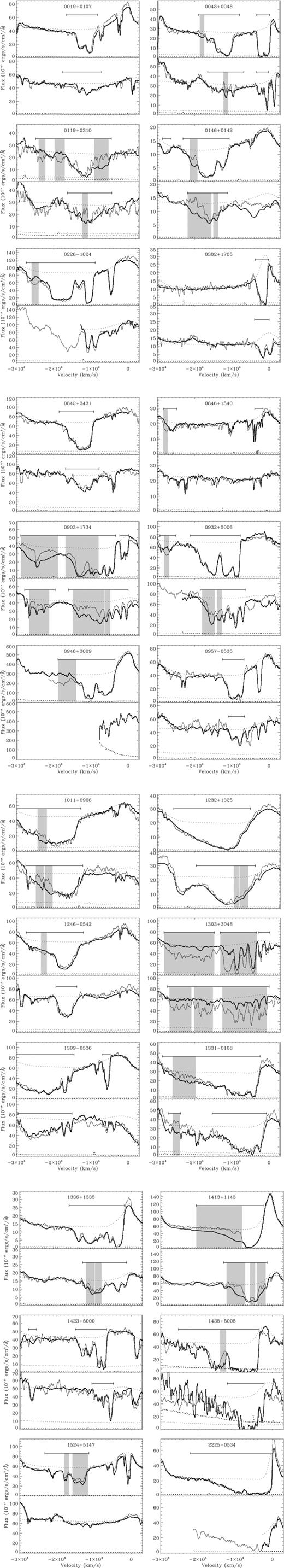
Spectra of all 24 quasars in our sample, showing the long-term comparisons (Δt= 3.8–7.7 yr) between a Lick Observatory spectrum (bold curves) and a recent MDM spectrum (thin curves). For each quasar, the C iv region is displayed in the top panel and the corresponding Si iv region is shown in the bottom panel. For 2225−0534, we only have short-term Lick data (see Table 1). The vertical flux scale applies to the Lick data, and the MDM spectrum has been scaled to match the Lick data in the continuum. The dashed curves show our pseudo-continuum fits. The horizontal bars indicate intervals of BAL absorption included in this study, and the shaded regions indicate intervals of variation within the BALs. We used binomial smoothing to improve the presentation of the spectra. The formal 1σ errors are shown near the bottom of each panel. (The two variability intervals defined for 1524+5147 were labelled as one interval in Paper 1.).
We adopt the velocity ranges over which C iv BAL absorption occurs defined in Paper 1. These regions were defined based on the definition of BI, i.e. they must contain contiguous absorption that reaches ≥10 per cent below the continuum across ≥2000 km s−1. We apply the same definition when defining the velocity ranges of Si iv BAL absorption.
In Paper 1, we defined a pseudo-continuum fit for the fiducial Lick observation used in the long-term analysis for each quasar by fitting a power law to regions of the spectrum free of absorption and emission. The preferred spectral regions for the fits were 1270–1350 and 1680–1800 Å, but were adjusted to avoid emission and absorption features as much as possible or due to the limits of the wavelength coverage. We then fit the C iv emission lines, using between one and three Gaussians to define the line profile. In Paper 1, we also fit the Si iv emission in cases where C iv absorption overlaps with the Si iv emission. For this work, we additionally fit the Si iv emission in the fiducial Lick observation for all the quasars. For the long-term comparisons below, we fit the Si iv emission for the MDM spectrum in cases where the emission line varied. Some special cases where there were difficulties with fitting the Si iv emission, such as 1011+0906 and 1309−0536, are discussed further in Section 3.3 below.
When comparing multiple epochs, we scaled all the spectra to the fiducial Lick spectrum used for the pseudo-continuum fit. We only fit the power-law continuum to one spectrum for each object, so any errors in this continuum fit will not effect our main variability results. To match the individual epochs for each quasar, we adopt a simple vertical scaling that matches the spectra along the continuum redwards of the C iv emission line (i.e. from 1560 Å to the limit of the wavelength coverage), between the Si iv and C iv emission (∼1425–1515 Å), and between the Lyα and the Si iv emission (∼1305–1315 Å). For the few cases where a simple scaling did not produce a good match and there were disparities in the overall spectral shape between the comparison spectra, we fit either a linear function (for 0903+1734, 1413+1143, 1423+5000 and 1524+5147) or quadratic function (for 0019+0107 and 1309−0536) to the ratio of the two spectra across regions that avoid the BALs. We then multiplied this function by the SDSS or MDM spectrum to match the fiducial Lick data.
However, photon statistics alone are not sufficient for defining real variability, so we took a conservative approach, described in more detail in Paper 1, whereby we omit ambiguous cases of variability, even if they meet the 4σ threshold. Flux calibrations, a poorly constrained continuum placement and underlying emission-line variability can all add additional uncertainty to identifying variability. For example, in 1011+0906 and 1309−0536, there might be BAL absorption, and variability, on top of the Si iv emission line (see Fig. 1). However, it is too ambiguous to be included in this study. See Paper 1 for further examples of intervals of potential variability that were not included because of additional uncertainties and Section 3.3 below, where we comment further on certain individual quasars. We include narrow intervals of variability such as the shaded region in Si iv in 0043+0048 and the shaded region in C iv in 1246−0542 in Fig. 1, where the flux differences are 6.3σ and 5.6σ, respectively. These regions meet the aforementioned thresholds, and the comparison spectra match well in regions of the continuum free of emission and absorption and on either side of the variability interval. We also include regions such as those shaded in 1011+0906 in Fig. 1 because even though the errors are slightly higher in the MDM spectra shown, the flux differences are still 7.7σ for the variable region in C iv and 6.3σ and 7.9σ for the two regions of variability in Si iv. Overall our approach is designed to be conservative; we try to exclude marginal cases of variability to avoid overestimating the true variability fractions.
We calculated the absorption strength, A, of the BALs in our sample, where A is the fraction of the normalized continuum flux removed by absorption (0 ≤A≤ 1) within a specified velocity interval. These calculations are described in Paper 1. Very briefly, we divide each interval of variability and absorption, as defined above, into equal-sized bins of width 1000–2000 km s−1, with the final bin size depending on the total velocity width of the specified interval. Then, for each quasar, we adopt the same bin size for the epochs being compared and calculate 〈A〉 and ΔA in every individual bin.
One of the difficulties in directly comparing C iv to Si iv absorption is the wider doublet separation in Si iv (500 km s−1 in C iv versus 1900 km s−1 in Si iv). This can cause the Si iv absorption intervals to be wider than those in C iv. The only effect this should have on the variability results in Section 3 below is that there may be portions of Si iv absorption that are detected as variable but the corresponding velocity intervals in C iv may be too narrow to pass our variability threshold. We comment further on this in Section 3.1. We mark the regions defined as BAL absorption (horizontal bars) and variability (shaded rectangles) in Fig. 1. The absorption and variability regions for C iv were defined in Paper 1. We defined the absorption and variability regions for Si iv independently from what we found for C iv. See Section 3.1 for a full discussion of these results.
In Fig. 2, we plot the relationship between absorption strength, 〈A〉, in C iv and 〈A〉 in Si iv for the long-term spectra shown in Fig. 1. Each point represents a different absorption bin in an individual quasar, such that individual quasars contribute multiple points to this plot. The diagonal line through the plot represents equal strength in both lines. Since we fix the velocity scale based on the bluer doublet member in C iv and in Si iv and the doublet separation is wider in Si iv, the edges of the Si iv absorption troughs tend to extend redwards of the edges of the corresponding C iv troughs (see, for example, 0302+1705 in Fig. 1). As mentioned above, to calculate the 〈A〉 values, we divide each BAL into bins. We thus remove the redmost bin for each absorption trough because Si iv may have a greater strength than C iv in those bins due to the wider doublet separation and not necessarily because the Si iv absorption is actually stronger than C iv. We also plot 1σ error bars, calculated by using the error spectra shown in Fig. 1 and averaging over the velocity interval for each bin. We point out that non-statistical errors, e.g. from the continuum fitting, can increase the error in 〈A〉 measurements by up to 0.05–0.1. It is clear from Fig. 2 that absorption in C iv is roughly as strong or stronger than the corresponding Si iv absorption. In some cases, the C iv has no detectable corresponding Si iv absorption at all.
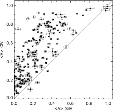
The average normalized absorption strength, 〈A〉, in C iv versus the 〈A〉 in Si iv for each absorption bin in each quasar in the long-term subsample. The error bars represent the 1σ errors based on photon statistics.
There are almost no well-measured cases of C iv absorption weaker than Si iv. We did find a few absorption bins where Si iv appeared to be stronger than C iv, but some of these bins might not actually have absorption due to Si iv, or due solely to Si iv. In about 10 per cent of BAL spectra, there are lower ionization lines, such as C iiλ1335 and Al iiiλ1855,1863 (Trump et al. 2006). The wavelength of C ii places any C ii absorption line at a velocity of <−13 500 km s−1 in Si iv velocity space. In order to look for interloping C ii lines, we checked all of our objects for another low-ionization species, Al iii, which exists redwards of C iv, in a region of the spectrum relatively uncontaminated by other lines. We found that in two cases (1232+1325, 1331−0108), the velocity of the Al iii line puts the corresponding C ii line within a Si iv BAL trough. We therefore removed the bins affected by C ii from Fig. 2, and we exclude the contaminated Si iv regions in these two quasars from the analysis below. There are still a few points below the one-to-one line in Fig. 2. However, these few points are mostly within 3σ of the one-to-one line and therefore are consistent with equal strength changes in C iv and Si iv. The one point that is just beyond 3σ from the line corresponds to the interval −3100 to −1200 km s−1 in 1303+3048.
3 RESULTS
3.1 Variability in Si iv versus C iv BALs
In this section, we directly compare the variability of Si iv to C iv in the ‘long-term’ data set from Paper 1. This involves two epochs of data for 23 quasars separated by 3.8–7.7 yr. Our main goal is to discriminate between the possible causes of BAL variability. We begin by looking at what fractions of quasars exhibited C iv and Si iv variability to determine if Si iv varies more or less often than C iv. In Paper 1, we found a correlation between the incidence of C iv BAL variability and outflow velocity and absorption strength. Here we investigate whether similar trends exists for Si iv BALs. We then look at the relationship between the incidence of C iv variability and Si iv strength. Last, we compare the change in strength for the two lines when they both vary.
In the long-term data set in Paper 1, 15 out of 23 quasars (65 per cent) exhibited C iv BAL variability and 11 out of 19 (58 per cent) exhibited Si iv BAL variability, at any measured velocity. We do not have data covering the Si iv region for two of our quasars, and another two quasars do not have Si iv BALs. This comparison between C iv and Si iv is complicated because the absorption in C iv is not always accompanied by corresponding absorption (e.g. at the same velocities) in Si iv (Figs. 1 and 2). In addition, we are observationally less sensitive to absorption and variability at high velocities in Si iv, compared to C iv, because those wavelengths can have poorer signal-to-noise ratios and larger uncertainties in the continuum placement caused by blends with underlying broad emission lines (BELs). Altogether, this means we are more sensitive to variability in C iv than Si iv in our data set.
To make a fair comparison between the incidence of variability in the two lines, we recalculate the above fractions while considering just the flow speeds at >−20 000 km s−1. We adopt this velocity as the cut-off because, in some spectra, there is emission due to O i at ∼−20 500 km s−1 in the Si iv absorption region (see also Gibson et al. 2010). With this additional restriction, we find that Si iv is more likely to vary than C iv. In particular, 35 per cent (8/23) of quasars exhibited C iv variability and 47 per cent (9/19) exhibited Si iv variability. The dramatic reduction in the C iv variability recorded this way, compared to the 65 per cent quoted above, is due to (i) consideration of a narrower velocity range and (ii) the specific exclusion of high velocities, which are the most likely to show variability (Paper 1). Nearly half of the occurrences of C iv variability detected in our data set are at high velocities, i.e. v <−20 000 km s−1. The incidence of C iv variability further reduces to 31 per cent (6/19) if we only include the 19 quasars which have complete spectral coverage across Si iv and have a Si iv BAL. The further decline in the C iv variability in this case probably occurs because the two quasars excluded for having no Si iv BAL have weak C iv lines, and weak C iv lines are more likely to vary than strong ones (Paper 1). Thus, we again removed C iv BALs that are more likely to vary.
Overall, it is important to realize that a number of factors can affect the measured incidence of BAL variability. Our comparisons show that, over matching velocity ranges, Si iv BALs have a significantly higher incidence of variability than C iv BALs. This difference is probably related to the different line strengths. In particular, the Si iv BALs are generally weaker than C iv BALs (Fig. 2), and weaker lines tend to be more variable (Paper 1 and Figs 4 and 5 below).
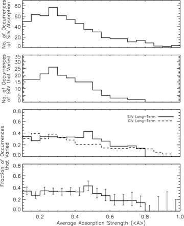
The top two panels show the number of occurrences of Si iv BAL absorption and variability versus the average normalized absorption strength, 〈A〉, in Si iv. The third panel is the second panel divided by the first. The bottom panel shows the same curve from the third panel with 1σ error bars overplotted.
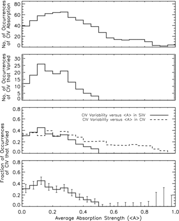
The top two panels show the number of occurrences of C iv BAL absorption and variability versus the average normalized absorption strength, 〈A〉, at the same velocities in Si iv. The third panel is the second panel divided by the first, and the bottom panel shows the same curve from the third panel with 1σ error bars. In the third panel, we overplot the fraction of occurrences of C iv absorption that varied versus 〈A〉 in C iv.
To more directly compare Si iv and C iv BAL variability, we examine the individual velocity intervals over which the variability occurs. We consider intervals at all velocities here and in the remainder of this section. Variability in C iv occurred in a total of 20 velocity intervals. 10 of these intervals have measurable Si iv absorption. Nine of these 10 intervals, or 90 per cent, showed Si iv variations in the same sense (either getting stronger or weaker) as the C iv changes. There is only one interval (in 0119+0310) that exhibits variability in C iv, without corresponding variability at the same velocities in Si iv. Conversely, we find long-term Si iv BAL variability in a total of 22 velocity intervals. All of the variable Si iv intervals have significant corresponding C iv absorption, and 10 of these intervals showed C iv variations in the same sense as the Si iv (45 per cent).
As mentioned in Section 2.2, Si iv has a wider doublet separation than C iv, causing some of the Si iv absorption and variability intervals to be wider than the corresponding C iv intervals. For the intervals of Si iv variability without corresponding C iv variability, we looked for any evidence of variability in C iv that was not included because the width of the candidate varying region was too narrow to meet our variability threshold (see Section 2.2). There is only one case where we detect a marginal narrow variability region in C iv corresponding to a region in Si iv classified as variable (in 0903+1734). Even if we were to count this as a variable C iv interval, still only 50 per cent of Si iv variability intervals would have corresponding C iv variability. Therefore, while 91 per cent of the intervals of C iv variability had corresponding Si iv variability, only ∼50 per cent of the intervals of Si iv variability had corresponding C iv variability. These results reinforce our main conclusion above that Si iv BALs are more likely to vary than their C iv counterparts.
Next we examine the dependence of Si iv variability on velocity and absorption strength, matching our analysis of C iv BALs in Paper 1. Fig. 3 shows the incidence of Si iv absorption and Si iv variability versus velocity. For comparison, this figure also shows the corresponding data for C iv taken directly from fig. 3 in Paper 1 (dashed curves). The top two panels display the number of quasars with Si iv BAL absorption and with Si iv BAL variability at each velocity (solid curves). The third panel is the second panel divided by the top one, which gives the fraction of Si iv BALs that varied at each velocity. The top panel shows clearly that there are more C iv BALs than Si iv BALs at higher velocities.
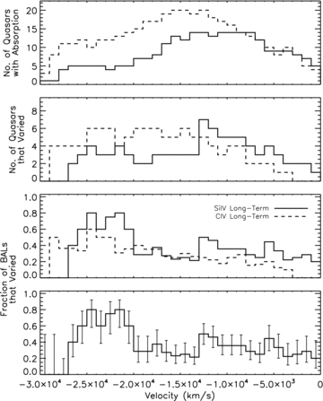
The top two panels show the number of occurrences of Si iv (solid lines) and C iv (dashed lines) BAL absorption and variable absorption versus velocity. The third panel is the second panel divided by the first. The bottom panel shows the same curve from the third panel for Si iv with 1σ error bars.
In Paper 1, we showed that the incidence of C iv variability increases significantly with increasing velocity. This trend is not evident in the Si iv data. Fig. 3 displays 1σ error bars based on Wilson (1927) and Agresti & Coull (1998). These errors are based on counting statistics for the number of quasars with absorption and variability at each velocity. We performed a least-squares fit, and the slope of the Si iv data is −6.58 ± 4.33 × 10⁻⁶, in the formal unit, fraction per km s−1. The slope is non-zero at just a 1.5σ significance. Therefore, while there might be a weak tendency for more variability in Si iv at higher velocities (Fig. 3), the trend is not statistically significant.
To further match our analysis from Paper 1, we looked at the relationship between the incidence of Si iv variability and the absorption strength, 〈A〉, in Si iv. As described in Paper 1 (and Section 2 above), we divide each BAL into ∼1200 km s−1 bins, and we treat each bin as an individual occurrence of absorption. In Fig. 4, the top two panels show the number of these occurrences of Si iv absorption and the number of these occurrences that varied at each value of Si iv absorption strength, 〈A〉. An individual quasar can contribute more than once to each point in the histogram. The third panel is the second panel divided by the top one, and the bottom panel shows the same curve from the third panel with error bars plotted, calculated in the same way as for Fig. 3. We find only a weak trend between Si iv variability and Si iv strength. The slope of the plot is −0.315 ± 0.090 fraction per unit absorption strength, which is non-zero at a 3.5σ significance. This is much weaker than the trend between the incidence of C iv variability and C iv strength found in Paper 1. We overplot this curve for C iv from fig. 5 of Paper 1 in the third panel of Fig. 4 (dashed curve). This indicates that the occurrence of variability in Si iv is less sensitive to the strength of the line than the occurrence of variability in C iv.
Next, we looked at the relationship between the incidence of C iv BAL variability and the strength of the Si iv absorption, 〈A〉, at the same velocities. Si is known to be less abundant than C, when solar abundances are assumed, and the high ionization typical in BALs favours C iv (see Section 5). Therefore, the optical depth in C iv is higher than in Si iv, so the stronger the Si iv absorption is, the more likely C iv is to be saturated. In Fig. 5, we plot the number of occurrences of C iv absorption that occur at the same velocities in the same spectra as each Si iv〈A〉 value and then the number of these occurrences that varied in the second panel. As in Fig. 4, an individual quasar can contribute more than once to each point in the histogram. The third panel is the second panel divided by the top one, showing the fraction of occurrences of C iv absorption that varied at each Si iv absorption strength value. As in Figs 3 and 4, the bottom panel of Fig. 5 shows the 1σ error bars. The slope of these points is −0.643 ± 0.066 fraction per unit absorption strength, which is non-zero at a 10σ significance. Fig. 5 thus indicates that the incidence of C iv variability decreases with increasing Si iv absorption strength. Therefore, when the Si iv absorption is stronger and the C iv absorption is more likely to be saturated, the incidence of C iv variability decreases. In fact, whenever the Si iv absorption strength is greater than 0.5, the corresponding C iv absorption at the same velocity does not vary.
As a further comparison to Paper 1, we overplot in the third panel of Fig. 5 the fraction of occurrences of C iv absorption that varied versus C iv absorption strength (dashed curve). In Paper 1, we concluded that, for C iv BALs, weaker lines are more likely to vary than stronger lines. Fig. 5 shows that C iv lines are even more likely to vary when the corresponding Si iv lines are also weak.
We also investigate the change in strength, |ΔA|, in C iv compared to the corresponding changes in Si iv in the same velocity interval (Fig. 6). There are six quasars in which the velocity intervals of C iv and Si iv variability overlap, and we only compare the velocity intervals where both lines varied. Each point represents one bin in one of these quasars, as described above for Fig. 5. The diagonal line through this plot corresponds to equal strength changes in both lines. There is clearly no correlation between the strength changes in C iv versus Si iv evident in this figure. Despite Si iv varying more often than C iv, the strength changes in Si iv are not always greater than in C iv.
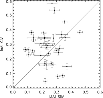
The change in strength of C iv BAL absorption versus the change in strength of Si iv BAL absorption in velocity intervals where both lines varied. The error bars are calculated as in Fig. 2.
Finally, Fig. 7 shows the fractional change in strength, |ΔA|/〈A〉, in C iv compared to |ΔA|/〈A〉 in Si iv, again for velocity intervals where both lines varied. As in Fig. 6, there are points lying above the line, representing greater strength changes in C iv than in Si iv. However, there is a weak trend towards greater fractional change in strength in Si iv, which is consistent with the correlation found between fractional change in EW in C iv and Si iv in Gibson et al. (2010).
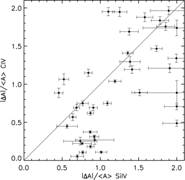
The fractional change in strength of C iv BAL absorption versus the fractional change in strength of Si iv BAL absorption in velocity intervals where both lines varied. The error bars are calculated as in Fig. 2.
As mentioned in Section 2.1, we include two quasars that have BI =0 because they do have broad absorption, but it falls outside the velocity range, −25 000 to −3000 km s−1, used in the strict definition of BI. We also include broad absorption in other quasars in our sample that falls outside of this velocity range. Their inclusion has minimal impact on our results because most of the Si iv broad absorption in our sample falls within this velocity range. For the quasars with BI =0, 0846+1540 does not contain any Si iv broad absorption at all, and 0302+1705 contains broad absorption at low velocity, which did not vary in either C iv or Si iv.
We can summarize our comparisons between the C iv and Si iv BAL variabilities as follows: (1) Si iv BALs are more likely to vary than C iv BALs. The fractions of quasars showing variability in our long-term two-epoch data set are 31 per cent in C iv and 47 per cent in Si iv if we consider only the well-measured velocity range v > −20 000 km s−1 and include only quasars with both Si iv and C iv BALs detected. (2) The variabilities usually occur in just portions of the BAL troughs. (3) When changes occur in both Si iv and C iv, they always occur in the same sense (i.e. with both lines getting either weaker or stronger). They also occur in overlapping but not necessarily identical velocity ranges. (4) The trend for a higher incidence of C iv variability at higher velocities, which we reported in Paper 1, is not clearly evident in the Si iv data. (5) Finally, there is no correlation between absorption strength changes in C iv versus Si iv when they both vary; although, there is a weak trend towards greater fractional change in strength in Si iv.
3.2 Multi-epoch monitoring of BALQSOs
We now expand our analysis to the full data set, which includes 2–10 epochs of data for each object (Table 1). Including all of these epochs and considering all measured velocities, the fraction of quasars that showed C iv BAL variability is 83 per cent. This is a significant increase from the 65 per cent we derived considering only two long-term epochs, or the 39 per cent derived from only two short-term epochs (Section 3.1 and Paper 1). Clearly, including more epochs of data increases the observed variability fractions. Moreover, these larger variability fractions apply to roughly the same time frame as our two-epoch long-term data set. Therefore, the multi-epoch data did not find new occurrences of variability at some other time; they identified variability missed by the two-epoch measurements.
To investigate the multi-epoch behaviours of BAL variability, we compared all the spectra obtained for each quasar. From one object to another, there are large differences in the widths of the varying regions and the amplitudes of the changes (e.g. see Figs 1 and 6). However, there are certain general trends that most, if not all, of the quasars follow. In particular, the variability almost always occurred within just a portion of a BAL and not in the entire trough. In nearly all the quasars, the variability occurred over the same velocity interval(s) between each epoch. Finally, when there are multiple velocity intervals of variability within the same quasar, the changes in these separate intervals almost always occur in the same sense. Similarly, as described in Section 3.1, when there is variability in both C iv and Si iv, they also vary in the same sense.
We also find no clear evidence for velocity shifts that would be indicative of acceleration or deceleration in the flows. The constraints on velocity shifts are difficult to quantify in BALs because there can be complex profile variabilities, but we specifically search for and did not find cases where a distinct absorption feature preserved its identity while shifting in velocity. Despite the large outflow velocities, there is no clear evidence to date for acceleration or deceleration in BALs, or in any other outflow lines [i.e. narrow absorption lines (NALs) and mini-BALs; e.g. Rodríguez Hidalgo et al. 2011].
We highlight below a few well-sampled cases to illustrate these general trends in the data. Fig. 8 shows specifically the quasars for which we have at least seven measured epochs including one from the SDSS, which helps to span the time gap between the early Lick data and our recent MDM observations. For each object, the top panel shows the C iv BAL(s) and the bottom panel shows the Si iv BAL(s). The blue curves show the early Lick data, the red curves show the intermediate SDSS data and the green curves show the MDM spectra. We note that in 1524+5147 there is an O i emission line centred at ∼−20 500 km s−1 in the Si iv panel.
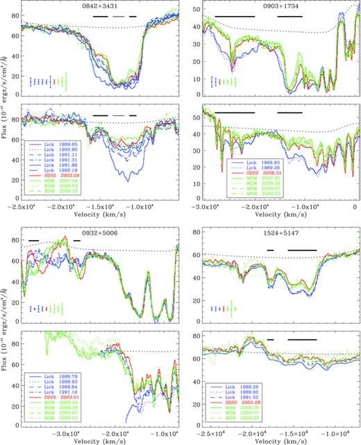
Spectra of the C iv (top panel) and Si iv (bottom panel) BALs in four well-sampled quasars from our sample, after smoothing three times with a binomial function. The blue curves are the Lick spectra, red curves are SDSS spectra and green curves are MDM spectra. The bold bars mark varying regions identified for C iv. The average error for each spectrum is shown in the top panel for each quasar, where the height of the error bar represents ±1σ.
The bold bars in Fig. 8 mark intervals of variability identified for C iv. The velocity ranges are guided by the intervals defined for C iv in Paper 1 and are adjusted to cover the core of the varying region and avoid the edges where the variability is less pronounced. These same velocity ranges are applied to all the epochs plotted here and to Si iv for comparison. The one exception is the thin bar marking a region of variability in Si iv in 0842+3431 with minimal corresponding variability in C iv. For all of these varying regions, we calculate the absorption strength, A, for the defined velocity intervals in each epoch and then plot these A values versus time in Fig. 9.
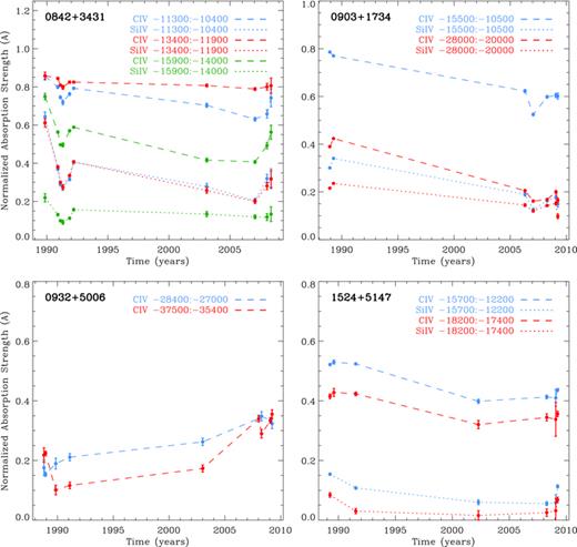
The absorption strength in both C iv (dashed lines) and Si iv (dotted lines) as a function of time in the velocity intervals indicated by bars in Fig. 8.
We plot A instead of EW, in Fig. 9, in order to highlight the intervals that varied. Using EW would dilute these changes in strength. The different colours correspond to different velocity intervals. The dashed and dotted lines represent changes in C iv and Si iv, respectively. We note that these lines do not represent how the A values changed between epochs. They simply connect the measurements from different epochs in order to aid the eye.
In Fig. 8, the spectra of 0842+3431 (in the C iv BAL), 0903+1734 and 1524+5147 show clearly how portions of BALs can vary. In 0842+3431, there is significant variability in both the blue side and the red side of the C iv BAL; although in Si iv, the entire BAL varies (see Section 3.3.3 below). In 0903+1734, there is significant variability at higher outflow velocities, but at lower velocities, there is no variability. This is consistent with the result from Paper 1 that there is a higher incidence of variability at higher velocities. The variable regions in 1524+5147 cover most, but not all, of the BAL. In contrast to the general trends in Paper 1, the bluemost portion of the BAL did not vary. In 0932+5006, however, the entire C iv BALs vary at the highest velocities. In terms of C iv to Si iv comparisons, 1524+5147 is a case where there is weak corresponding absorption, and variability, in Si iv, but no Si iv BAL. And, 0932+5006 shows clearly a case where a Si iv BAL varied, but the C iv BAL did not.
The plots in Fig. 9 for 0842+3431, 0903+1734 and 0932+5006 show how the change in A is not always monotonic. The same BAL can grow deeper from one epoch to another, then become shallower again. This is consistent with the results of Gibson et al. (2010). Furthermore, the change in the A value from one epoch to another generally occurs in the same direction (either positive or negative) in both C iv and Si iv, which is consistent with the results of Section 3.1. In 0842+3431, 0903+1734 and 1524+5147, where there are two separate intervals of C iv variability, the change in strength occurs in the same direction for both intervals. The high-velocity BALs in 0932+5006 vary in concert starting with the 1989.84 epoch through 2008.03. At the earliest and latest epochs, they do not clearly vary in concert, but the changes in A are small and could be affected by changes in the underlying Si iv emission line. We comment further on these BALs in 0932+5006 in Section 3.3.4.
3.3 Notes on individual quasars
In this section, we comment on individual quasars that are cases of special scientific interest. We also comment on cases where there were specific issues in the analysis or measurements that result in larger uncertainties.
3.3.1 0119+0310
0119+0310 is the only quasar for which we record C iv BAL variations without corresponding changes in Si iv in our long-term sample (Fig. 1 and Section 3.1). However, these results are very tentative because the Si iv absorption is poorly measured across the velocities that varied in C iv. The two long-term spectra for this object, plotted in Fig. 1, have a lower signal-to-noise ratio level than most of the other data in our sample. Furthermore, the Si iv absorption at the velocity of C iv variability (∼−7500 km s−1) is very weak, and if the continuum fit is off by even ∼5 per cent, this region in Si iv might not be considered part of the Si iv BAL. If this region is not part of the BAL, then we would not include it in the comparison of C iv to Si iv. Therefore, while we have several well-measured cases of Si iv variability without corresponding C iv variability, we only have this one poorly measured case of C iv variability with no corresponding Si iv variability.
This quasar also appears to differ from most of the other quasars in the sample in that the different regions of C iv variability do not vary in the same sense (Fig. 1). The two higher velocity variable regions both increase in strength between the Lick and MDM observations, while the lower velocity variable region decreases in strength. As mentioned above, this is one of our least well-measured quasars, so this is a tentative result. We find just two other cases where two regions of C iv variability vary in opposite directions (0146+0142 and 1423+5000).
3.3.2 0146+0142
We first note that this object has a high-velocity C iv BAL, so the BAL that appears just redwards of the marked Si iv BAL in Fig. 1 is actually C iv. As mentioned in Paper 1, we can confirm that this is high-velocity C iv, and not Si iv, because if it were Si iv absorption, we should see corresponding low-velocity C iv absorption (see also fig. 1, Korista et al. 1993). We also have further confirmation that this is high-velocity C iv absorption because we find evidence of corresponding high-velocity Si iv absorption on top of the Lyα emission line. Fig. 10 shows the two long-term spectra for 0146+0142 with the two rightmost shaded regions marking the C iv variability and the two leftmost shaded regions marking the corresponding velocities (but not necessarily the entire variable regions) in Si iv.
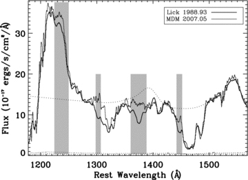
The two long-term epochs for 0146+0142, showing the full spectrum from the Lyα emission through the C iv emission. The shading here differs from Fig. 1, with the rightmost shaded regions marking the C iv variability and the leftmost shaded regions showing the corresponding velocities in Si iv (but not the exact regions of Si iv variability). This figure shows evidence of Si iv BAL variability on top of the Lyα emission line.
Another interesting note about 0146+0142 is that in our short-term data, there are two separate regions of C iv BAL variability, but they do not vary in the same sense. In Fig. 11, we plot the two short-term epochs with these two variable regions shaded. The redder varying interval at ∼−28 300 km s−1 increases in strength, while the bluer interval at ∼−36 600 km s−1 decreases in strength. As mentioned in Section 3.3.1, this is one of just three cases showing this behaviour.
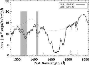
The two short-term epochs for 0146+0142, with the two shaded regions marking C iv variability. The absorption in these two regions varies in opposite directions, with one region becoming weaker while the other becomes stronger.
3.3.3 0842+3431
In 0842+3431, there is significant variability in two distinct regions of the C iv BAL trough (marked by bold bars in Fig. 8), while the entire Si iv trough varies. However, the bluer, and more variable, region in the C iv trough (the leftmost bold bar in Fig. 8) corresponds to a region of weak absorption and variability in Si iv. Some of the variability in the redmost portion of the Si iv trough (the rightmost bold bar in Fig. 8) may be connected with the variability in the red side of the C iv BAL trough, but the variability in the core of the Si iv trough, marked by the thin bar in Fig. 8, cannot be explained by the wider Si iv doublet separation alone. Some of the Si iv variability is occurring at different velocities from the C iv variability. Nonetheless, as seen in Fig. 9, the changes in strength in all three marked regions of the Si iv trough occur in the same sense as the changes in strength in the two distinct varying regions in C iv.
Another interesting note about 0842+3431 is that we identified it as variable in the short term, but not in the long term, in Paper 1. For the long-term comparison in Paper 1, we used the 1990.90 and the 2008.35 observations. However, Figs 8 and 9 clearly show that the C iv BAL varied. The strength of the BAL is weaker in 2007.04 than in 1990.90, but the BAL becomes stronger again by 2008.35. Therefore, when looking at just the 1990.90 and 2008.35 observations, it appears as if the BAL did not vary at all. This shows how variable profiles can return to a previous state and that variable BALs can be missed in two-epoch studies.
3.3.4 0932+5006
As in 0146+0142, we note that the absorption trough that appears just redwards of the Si iv BAL in 0932+5006 in Fig. 1 is actually a high-velocity C iv BAL (see Fig. 8).
In 0932+5006, there is C iv absorption overlapping Si iv emission. The variability in these two detectable BAL troughs has a different behaviour from the variability in the other quasars in our sample. When looking at the spectra (Fig. 8), the two high-velocity BALs in the 2003.01 spectrum appear to be offset in velocity from the BALs in the other epochs. While this could be indicative of a shift in velocity of the BALs, this apparent offset could also be due to part of the trough weakening while the other part strengthens. This complicates the measurement of A for Fig. 9 because any measurement of A in a fixed velocity interval for each of these two high-velocity BALs does not accurately represent how the line changed. Furthermore, the Si iv emission line itself could be variable, which complicates any analysis of C iv BAL variability in this velocity range.
3.3.5 0946+3009
0946+3009 is the one object in our sample with a redshift too low for our MDM spectra to cover the entire C iv region out to the Si iv emission line. The spectra only go as blue as ∼−19 000 km s−1. The absorption and variability regions that we define for this quasar do not extend all the way to the edge of the MDM spectrum in order to avoid any uncertainties there. The detection of variability in this quasar is secure because we have an additional MDM spectrum of this quasar that matches the MDM spectrum shown in Fig. 1.
3.3.6 1011+0906
As mentioned in Section 2.2, some of the quasars in our sample have low-ionization BALs. We searched for Al iii lines in our sample and used the velocity of the Al iii line to determine the location of C ii. 1011+0906 has an Al iii BAL, but the velocity of the absorption puts C ii bluewards of the Si iv absorption. Therefore, if there is any C ii absorption in this object, it does not affect our measurements of the Si iv BAL.
The Si iv BEL in this quasar is mostly absorbed by the C iv BAL. We fit the Si iv BEL using the procedure defined in Paper 1 for cases like this. We take the C iv fit, increase the full width at half-maximum (FWHM) based on the greater doublet separation in Si iv, and place it at the wavelength where the Si iv emission should be. However, there is still some slight emission bluewards of the Si iv BEL fit. This extra emission may be part of the wing of the Si iv BEL, or the underlying power-law continuum fit might be slightly too low. However, the Si iv BAL is located at a high enough velocity that any error in the Si iv BEL fit should have a negligible effect on our measurements of the BAL and its variability.
3.3.7 1232+1325
1232+1325 has an Al iii BAL which puts C ii within the Si iv region. The C ii BAL is in the velocity range −25 500 to −19 600 km s−1 (see also Fig. 1), and we omit these velocities from our analysis.
3.3.8 1303+3048
1303+3048 is a BALQSO that also contained a C iv mini-BAL at ∼−18 500 km s−1 when first observed at Lick (Fig. 1). We only have one Lick observation of this object, but the MDM observations show that the mini-BAL widened and increased in strength to become a BAL. A BAL emerges at the same velocities in Si iv as well. The lower velocity BAL in 1303+3048 is visible in C iv in the Lick data, but appears as only weak absorption in Si iv. However, between the Lick and MDM epochs, a Si iv BAL emerges and the variability in the Si iv absorption extends to lower velocities than the C iv variability. The variability at all velocities in this quasar in both C iv and Si iv occurs in the same sense; the absorption increases in strength.
3.3.9 1309−0536
As in 1011+0906, the Si iv BEL in 1309−0536 is heavily absorbed by a C iv BAL. We used the same procedure that we used for 1011+0906 to fit the Si iv BEL, and we found what appeared to be significant emission bluewards of the Si iv BEL fit. In this case, the underlying power-law continuum fit did not have the correct slope, so we made a slight adjustment to the continuum fit. Adjusting the power-law continuum fit caused on average an increase in A of ∼6 per cent throughout most of the C iv trough, compared to the measurements in Paper 1. The new Si iv BEL fit increased A at the highest velocities in C iv by up to a factor of 2. Even with this adjustment, there still appears to be some slight emission bluewards of the Si iv BEL fit, but, as in 1011+0906, the Si iv BAL in 1309−0536 is at a high enough velocity that errors in the emission fit should not have much effect on measurements of the BAL. This quasar also did not vary in either Si iv or C iv, so any measurement errors for this quasar will not affect any of our results comparing Si iv and C iv variability properties (e.g. Figs 6 or 7).
3.3.10 1331−0108
As in 1232+1325, 1331−0108 has an Al iii BAL at a velocity that places the corresponding C ii absorption within the Si iv BAL. We therefore omit the velocity range −23 800 to −15 300 km s−1 in the Si iv region from our analysis.
While analysing the Si iv region in 1331−0108, we noted that the pseudo-continuum fit defined in Paper 1 needed to be adjusted. Like 1309−0536, 1331−0108 has very broad BALs, which makes fitting a continuum difficult. The slope of the fit for 1331−0108 is now slightly steeper than the fit used in Paper 1, increasing the measured A values for C iv on average by just ∼7 per cent throughout most of the trough and up to ∼30 per cent at the highest velocities, where the absorption is much weaker.
3.3.11 1423+5000
1423+5000 is another quasar where there were two C iv BALs that varied, but one BAL increased in strength, while the other weakened. This quasar varied between the Lick and SDSS observations, but we did not detect any variability in the long-term analysis in Paper 1. 0119+0310, 0146+0142 and 1423+5000 are the only quasars in our sample where we see two separate varying regions in C iv that did not vary in the same sense.
3.3.12 1435+5005
1435+5005 has Al iii absorption that is either a weak BAL or strong mini-BAL. However, the velocity of the absorption places C ii bluewards of the Si iv absorption.
We also note that the signal-to-noise ratio level in the data for 1435+5005 decreases rapidly at bluer wavelengths. We therefore do not include the spectral region bluewards of −12 100 km s−1 in Si iv in our analysis in Section 3.1.
4 SUMMARY OF RESULTS
This is the second paper in a three-part series to analyse the BAL variabilities in a sample of 24 BALQSOs measured originally by Barlow (1993) at the Lick Observatory in 1988–1992. We supplement those data with spectra from the SDSS archives (for eight quasars) and our own measurements obtained at the MDM observatory (Table 1). In Paper 1 we discussed the variability properties of C ivλ1549 measured in just two epochs that span a ‘short-term’ (0.35–0.75 yr) and a ‘long-term’ (3.8–7.7 yr) time interval. Here we build upon that work by including our full multi-epoch data set for these same quasars and making detailed comparisons between the Si iv and C iv BAL behaviours. Our main results are the following.
BAL variability usually occurred in only portions of the BAL troughs (Paper 1; Section 3.3.2).
In the long-term interval, 65 per cent of the BALQSOs in our sample showed C iv BAL variability while only 39 per cent varied in the short term (Paper 1).
C iv variability occurs more often at higher velocities and in shallower absorption troughs (or shallower portions of absorption troughs; Paper 1).
In rare cases, BAL features appear, disappear, or change to or from narrower mini-BAL features (Paper 1; Section 3.3.8).
C iv BALs in our data are as strong or stronger than Si iv BALs at all velocities (in all well-measured cases; Fig. 2).
Si iv BALs are more likely to vary than C iv BALs. For example, when looking at flow speeds >−20 000 km s−1, 47 per cent of the quasars in our sample exhibited Si iv variability while 31 per cent exhibited C iv variability (Section 3.1). The greater variability in Si iv is likely due to a combination of items (3) and (5) above; weaker lines are more likely to vary and Si iv tends to be weaker than C iv.
Variability in Si iv can occur without corresponding changes in C iv at the same velocities. ∼50 per cent of the variable Si iv regions did not have corresponding C iv variability at the same velocities. However, in only one poorly measured case were changes in C iv not matched by Si iv (Sections 3.1 and 3.3.1).
At BAL velocities where both C iv and Si iv varied, the changes always occurred in the same sense (Section 3.1).
We do not find any correlation between the absolute change in strength in C iv and in Si iv (Fig. 6), but the fractional change in strength tends to be greater in Si iv than in C iv (Fig. 7).
When additional observing epochs are included (e.g. our full data set; Section 3.2), the fraction of C iv BALs that varied at any velocity increases from 65 to 83 per cent. This increase was caused by variations missed in the two-epoch comparisons in Paper 1.
BAL changes at different velocities in the same ion almost always occurred in the same sense (getting weaker or stronger) but not generally by the same amount (Section 3.2). We find just three cases that show evidence for one C iv BAL weakening while another strengthens within the same object (Sections 3.3.1, 3.3.2 and 3.3.11).
The multi-epoch data also show that the BAL changes across 0.04–8.2 yr in the rest frame were not generally monotonic (Section 3.2). Thus, the characteristic time-scale for significant line variations, and (perhaps) for structural changes in the outflows, is less than a few years.
With more epochs added, we still do not find clear evidence for acceleration or deceleration in the BAL outflows (Section 3.2).
5 DISCUSSION
The BAL variability data provide important constraints on the outflow physical properties. However, the information we derive depends critically on what causes the BAL variations. In this section we discuss pros and cons of two competing scenarios, namely (1) fluctuations in the far-UV continuum flux that cause global changes in the outflow ionization and (2) outflow clouds moving across our lines of sight to the quasar continuum source.
An important part of this discussion is the BAL optical depths, which can be much larger than they appear in the spectrum if the absorbers cover only part of the background light source (Hamann 1998; Hamann et al. 2008). Comparisons between the C ivλ1549 and Si ivλ1400 BALs can help because these lines probe slightly different ionizations with potentially very different line optical depths. For example, in a simple situation with solar abundances and an ion ratio equal to the abundance ratio, i.e. Si iv/C iv= Si/C, the optical depth in Si ivλ1400 would be ∼3.4 times less than C ivλ1549 (Hamann 1997; Hamann & Ferland 1999; Asplund et al. 2009). In actual BAL flows, the relative Si iv optical depth should be even lower because BAL ionization tends to be high and thus favours C iv. We cannot make specific comparisons without specific knowledge of the absorber ionizations. However, if we reasonably assume that the ionization is at least as high as that needed for a maximum C iv/C ratio (e.g. in a gas that is photoionized by the quasar and optically thin in the Lyman continuum – fig. A1 in Hamann et al. 2011), then the Si iv optical depths should be >8 times smaller than C iv.
5.1 Changing ionization
When there is variability in different velocity intervals within the same BAL or within multiple BALs in the same quasar, the changes almost always occur in the same sense (e.g. 0842+3431 and 0903+1734; Figs 8 and 9). Studies of NAL variability have observed multiple NALs in a given quasar varying in concert (Misawa et al. 2007; Hamann et al. 2011). Hamann et al. (2011) found coordinated line variations in five NAL systems in a single quasar. They argue that the most likely explanation for this is a global change in ionization. If there are changes in the ionizing flux incident on the entire outflow, then global changes in ionization should occur. While the connection between NALs and BALs is unclear, this argument can be applied to BALs as well. Absorbing regions at different velocities have different radial distances from the central SMBH. They are therefore spatially distinct, even if they are part of the same larger outflow structure. A change in covering fraction due to moving clouds is unlikely in cases such as 0842+3431 and 0903+1734 because it would require coordinated movements among multiple absorbing structures at different outflow velocities and radii.
To further investigate this scenario, for simplicity, we consider a system with homogeneous clouds outflowing from the accretion disc, with no transverse motion across our line of sight to the quasar. A change in ionization will cause the optical depths in the lines to change. As mentioned above, the optical depths in C iv are higher than in Si iv, so Si iv would be more susceptible to changes in ionization. Therefore, it is more likely for Si iv to vary than C iv in this scenario because C iv is more likely to be saturated. This generally matches our results since we find that Si iv is more variable than C iv. We find only one case of C iv variability unaccompanied by Si iv variability, and it is a very tentative result (Section 3.3.1).
This scenario becomes a little more complicated when considering that typically variability only occurs in portions of BAL troughs, rather than entire BAL troughs varying (Gibson et al. 2008; Paper 1). As mentioned above, a change in ionization should cause more global changes, rather than changes in small, discrete velocity intervals. It is possible that the variable regions in the troughs have moderate or low optical depths, while the non-variable sections are too saturated to respond to modest changes in the ionization and line optical depths. We have evidence from Paper 1 and Fig. 5 that weaker lines, or weaker portions of lines, are more likely to vary. However, we also found in Paper 1 that variability is more common at higher velocities, where the absorption tends to be weaker, so it is difficult to say whether it is the higher velocity or the weaker absorption strength that is the root cause of the variability. If it is true that weaker portions of lines, which are least likely to be saturated, are more likely to vary, regardless of outflow velocity, then this would support the changing ionization scenario.
However, if it is true that weaker portions of lines are less saturated and thus more likely to vary, it is unclear why, for example, the weak blue wing of the BAL trough in 0842+3431 does not vary. If changing ionization is causing the variability in this quasar, then the wings of the line must be saturated while the portions of the line adjacent to the wings are not saturated. There are other examples of similar behaviour. In 1524+5147, the strongest variability occurs in the deepest segment of the BAL, and there is weak or no variability in the weakest segments of the trough (Figs 1 and 8). Similarly, the variability in 1011+0906 occurred near the core of the line, while the wings did not vary (Fig. 1).
In order for changing ionization to cause variability in just the deepest portions of BAL troughs, as in the examples given above, there must be velocity-dependent covering fractions with velocity-dependent optical depths. In this way, even the weak wings can be highly saturated. There is evidence in the literature that both optical depth and covering fractions can have complex velocity-dependent behaviours (Barlow & Sargent 1997; Hamann et al. 1997, 2001; Ganguly et al. 1999; de Kool, Korista & Arav 2002; Gabel et al. 2005; Gabel, Arav & Kim 2006; Arav et al. 2008).
The true optical depths and covering fractions are difficult to measure for BALs. In our data, 1413+1143 provides direct evidence for velocity-dependent optical depths if the line variations are caused by ionization changes. At the core of the Si iv trough there are two dips at the Si iv doublet separation (Fig. 1). The doublet ratio is roughly one-to-one, indicating saturation at these velocities and therefore little or no sensitivity to changes in continuum flux. This part of the trough did not vary. However, this saturated doublet is surrounded by variability at higher and lower velocities in Si iv. In C iv, which should have generally larger optical depths, variability occurs only at higher velocities. This behaviour is at least suggestive of lower optical depths (non-saturated absorption) at the variable velocities.
One further piece of evidence for the changing ionization scenario comes from the multi-epoch data in Section 3.2, which show that changes in BAL strength are not necessarily monotonic (see also Gibson et al. 2010). In fact, in 0842+3431, the absorption trough varied, and then in our last MDM observation it returned to the same strength it had in one of the first Lick observations. In order for a change in covering fraction to have caused the variability in 0842+3431, the cloud movements would have to be repeatable, in addition to being coordinated at different velocities corresponding to different spatial locations. A change in ionization is a more likely explanation because continuum flux variations are not necessarily monotonic either (e.g. Barlow 1993).
If a change in ionization does indeed cause the variability we detect, then there should be a connection between changes in continuum flux and BAL variability. However, the results from previous studies have been mixed. Barlow (1993) found some evidence for a correlation between continuum variability and BAL variations, at least in certain individual quasars, while other studies have not found a strong correlation (Barlow et al. 1992; Lundgren et al. 2007; Gibson et al. 2008). However, all of these studies look at near-UV flux variations and little is known about the far-UV variability properties of luminous quasars. It is the far-UV flux that is the source of the ionizing radiation. Therefore, these results do not rule out ionization changes as a cause of BAL variability.
5.2 Changing covering fraction
While most of the evidence presented so far favours ionization changes, previous BAL variability studies, including Paper 1, have favoured changing covering fractions over ionization changes (Lundgren et al. 2007; Gibson et al. 2008; Hamann et al. 2008; Krongold et al. 2010; Hall et al. 2011). To investigate this possibility, we consider a simple scenario with clouds that have constant ionization and column density, but are moving across our line of sight. If C iv and Si iv have the same covering fraction, then C iv should be just as likely to vary as Si iv, which is inconsistent with the results of Section 3.1. Further, the change in strength in the two lines should be the same, which is contradicted by our results in Fig. 6 (see also Gibson et al. 2010). Hence, this simple scenario clearly does not match the results of this and previous work.
A more realistic scenario involves clouds that can have different covering fractions in C iv and Si iv (Barlow & Sargent 1997; Hamann et al. 1997, 2001; Ganguly et al. 1999; Gabel et al. 2005, 2006; Arav et al. 2008). Hamann et al. (2001) and Hamann & Sabra (2004) discuss simple schematics of inhomogeneous clouds that could lead to different covering fractions in different ions [see fig. 6 in Hamann et al. (2001) and fig. 2 in Hamann & Sabra (2004)]. Stronger transitions in more abundant ions can have a larger optical depth over a larger area in these schematic models. Thus, Si iv may trace a different area of the outflowing gas clouds from C iv.
If the C iv and Si iv lines are saturated, e.g. like the BALs in Hamann et al. (2008), then the strengths of the lines would be governed by the covering fractions in those lines. In this case, a smaller covering fraction in Si iv would be consistent with the results of Fig. 2, which shows that Si iv lines are generally weaker than C iv. If Si iv is tracing a smaller area of the gas cloud than C iv and this cloud is moving across our line of sight, then Si iv absorption would generally be more variable. Furthermore, if the covering fractions are different for each ion, then the change in covering fraction, as well as the fractional change in strength of the absorption lines, for each ion can also differ. This is consistent with Figs 6 and 7.
In Sections 3.3.1, 3.3.2 and 3.3.11, we report on three cases that show evidence of one BAL, or one portion of a BAL, strengthening while another weakens within the same quasar. This can be readily explained in a moving cloud scenario, for it is possible for clouds at different velocities to enter/leave our line of sight at different times. If one cloud enters our line of sight, while another is exiting, we would see one BAL strengthening while another weakens.
5.3 Conclusions
The higher variability fractions in Si iv versus C iv BALs and coordinated variabilities between absorption regions at different velocities in individual quasars support the scenario of global changes in the ionization of the outflowing gas causing the observed BAL variability. Furthermore, velocity-dependent covering fractions and optical depths could explain why in many cases we see variability in just portions of BAL troughs, rather than entire troughs varying. On the other hand, variability in portions of BAL troughs fits naturally in a scenario where movements of individual clouds, or substructures in the flow, are causing changes in covering fractions in the absorption lines. This scenario is also consistent with the main results of Section 3.1, assuming that Si iv has a smaller covering fraction than C iv.
In reality, changes in ionization and covering fractions could both be contributing to BAL variability. In our sample, there are quasars in which we observed no variability; there are quasars that varied in only one or two narrow velocity intervals; and there are yet other quasars with variations over a wide range in velocities. It is unlikely that one scenario is governing the changes in all of these quasars. Perhaps in quasars where the lines are more saturated, the lines are not susceptible to small changes in ionization, but can easily vary due to covering fraction changes. In other cases, where the lines have lower optical depth, a change in ionization can cause large changes over a wide range in velocities, possibly masking variations due to changes in covering fraction.
There are still some unanswered questions that our results from Paper 1, and the current work, raise. In particular, in Paper 1, we find correlations between incidence of C iv variability and both velocity and absorption strength. However, velocity and absorption strength are also correlated. If the trend is really with absorption strength, indicating that weaker lines, which are less likely to be saturated, are more variable, then this favours ionization changes. If the trend is with velocity, then the implications are more ambiguous, but it would be more consistent with the crossing cloud scenario. Clouds with higher outflow velocities are more likely to have greater transverse velocities as well.
There are also documented cases of BALs emerging where there had hitherto been no absorption (Hamann et al. 2008; Krongold et al. 2010) and, in this work, we report on a quasar (1303+3048; Section 3.3.8) where a mini-BAL became a BAL. These scenarios speak to the general complexity of BAL variability. Previous studies have hypothesized that different outflow lines may indicate different inclinations of our lines of sight to the quasars and that at certain inclinations no absorption is seen (Elvis 2000; Ganguly et al. 2001). The connection between BALs, mini-BALs and NALs is still unclear. If BAL and mini-BAL outflows occur at different inclinations, then perhaps our line of sight to 1303+3048 goes through a region of overlap between the mini-BAL and BAL inclinations. One might expect this putative border region between the BAL and mini-BAL parts of the flow to be the most turbulent or unstable, and thus the most prone to showing line variability caused by structural changes/motions in the flow.
This work is only the second paper in a three-part series on BAL variability. The next paper will include (1) a more thorough exploration of the variability time-scales, with new data added to give extensive coverage across week to month intervals and (2) a more complete discussion of the implications of variability, e.g. in terms of the size, location and stability of outflow structures.
We thank an anonymous referee for helpful comments on the manuscript. Funding for the SDSS and SDSS-II has been provided by the Alfred P. Sloan Foundation, the Participating Institutions, the National Science Foundation, the US Department of Energy, the National Aeronautics and Space Administration, the Japanese Monbukagakusho, the Max Planck Society and the Higher Education Funding Council for England. The SDSS website is http://www.sdss.org/.
Footnotes
Throughout this paper, all time intervals are measured in years in the rest frame of the quasar.
The values of zem were obtained from the NASA/IPAC Extragalactic Database (NED), which is operated by the Jet Propulsion Laboratory, California Institute of Technology, under contract with the National Aeronautics and Space Administration.
REFERENCES
