Constraints on the ICM velocity power spectrum from the X-ray lines width and shift

Abstract

1 INTRODUCTION

Properties of gas motions in the hot intracluster medium (ICM) are still little known. It is believed that turbulent motions are driven when matter accretes on to the filaments or during shocks in the hot gas. Turbulence transfers kinetic energy injected on large scales L∼ Mpc to small (unknown) dissipative scales l. These two scales are connected with a cascade of kinetic energy, which occurs over inertial range (Kolmogorov 1941; Landau & Lifshitz 1966).

Knowing the properties of gas motions in clusters, we would be able to address a number of important question, e.g. what is the bias in the cluster mass measurements based on hydrostatic equilibrium and whether the bias is due to the motions alone or due to the clumping in gas density (see e.g. Rasia et al. 2006; Nagai, Vikhlinin & Kravtsov 2007; Jeltema et al. 2008; Lau, Kravtsov & Nagai 2009), what is the ICM turbulent heating rate in clusters (e.g. Churazov et al. 2008) and what is the role of gas motions in particle acceleration (see e.g. Brunetti 2006; Brunetti & Lazarian 2011).

Properties of turbulence in galaxy clusters were studied by means of numerical simulations (e.g. Norman & Bryan 1999; Cassano & Brunetti 2005; Dolag et al. 2005; Iapichino et al. 2011; Vazza et al. 2011). However despite the good ‘global’ agreement between all simulations, the results on turbulent motions are still controversial, mainly due to insufficient resolution of simulations and, in particular, low Reynolds number (effective Re < 1000 in cosmological simulations) and other numerical issues (see e.g. Dobler et al. 2003; Beresnyak & Lazarian 2009; Kitsionas et al. 2009).

Current generation of X-ray observatories cannot provide robust direct measurements of turbulence in the ICM. Only reflecting grating spectrometer on the XMM-Newton satellite (XMM RGS) can provide weak upper limits on velocity amplitude in cool core clusters (Sanders, Fabian & Smith 2011). Indirect indications of the ICM turbulence come from measurements of the resonant scattering effect (e.g. Churazov et al. 2004; Werner et al. 2009), from measurements of pressure fluctuations (Schuecker et al. 2004) or from surface brightness fluctuations (Churazov et al. 2012).

Future X-ray observatories, such as Astro-H1 and ATHENA,2 with their high energy resolution will allow us to measure shifts and broadening of individual lines in spectra of galaxy clusters with high accuracy. Combination of direct measurements of velocity amplitudes with indirect measurements via resonant scattering will give us constraints on anisotropy of motions (Zhuravleva et al. 2011). X-ray polarimetric measurements can also provide information on gas motions perpendicular to the line of sight (Zhuravleva et al. 2010).

Here we discuss the possibility of getting information about the length scales of gas motions (e.g. the size of energy-containing eddies). We discuss various ways to constrain structure function (SF) and power spectrum of gas motions via measurement of the projected velocity (shift of the line centroid) and the velocity dispersion (broadening of the line) as a function of projected distance from the cluster centre. These ideas are illustrated with a very simple model of a galaxy cluster. An application of our methods to simulated galaxy clusters will be considered in future work.

A similar problem of obtaining the SF of turbulence from spectral observations has been addressed in the studies of Galactic interstellar medium. In particular, it was shown that the width of molecular spectral lines increases with the size of a cloud (see e.g. Myers et al. 1978; Heyer & Brunt 2004; Heyer et al. 2009). This correlation was interpreted in terms of turbulent velocity spectrum (Larson 1981). A way to constrain SF of turbulence in the interstellar medium (ISM) by means of the velocity centroids (projected mean velocity) measurements was first considered by von Hoerner (1951) and Münch (1958) (see also Kleiner & Dickman 1983, 1985). Currently several different types of the velocity centroids method are used for studies of the ISM turbulence (see e.g. Esquivel et al. 2007). More advanced techniques, such as Velocity Channel Analysis (VCA) and Velocity Coordinate Spectrum (VCS) (see e.g. Lazarian & Pogosyan 2000, 2008; Chepurnov & Lazarian 2009), were developed and applied to the ISM data in the Milky Way and other galaxies (see e.g. Stanimirović & Lazarian 2001; Padoan et al. 2009; Chepurnov et al. 2010). Few other methods were also used, among them are the Spectral Correlation Function (SCF) (Rosolowsky et al. 1999; Padoan, Goodman & Juvela 2003) and the principal component analysis (PCA; Brunt et al. 2003).

The ISM turbulence is often supersonic and compressible (e.g. Elmegreen & Scalo 2004). This leads to (i) large shifts in the energy centroid of the line compared to the thermal broadening and (ii) large amplitude of the gas density fluctuations. At the same time individual lines, which are used to study the ISM turbulence (e.g. 21 cm line of H i or CO lines), are often well separated from other emission lines. The regions under study often have very irregular structure on a variety of spatial scales. The analysis therefore is usually concentrated on separation of the velocity and density fluctuations in the observed data, while the thermal broadening can often be neglected.

In contrast, in galaxy clusters the gas motions are mostly subsonic. The detection of the gas motions is still possible, since we deal with the emission lines of ions of heavy elements like Fe, Ca or S. The atomic weights of these elements are large (e.g. for Fe it is 56) and this drives pure thermal broadening of lines down (see Fig. 1 and Section 7.2). The brightest lines in spectra of galaxy clusters are often very close to each other. For example, in the vicinity of the He-like iron line at 6.7 keV there are forbidden and intercombination lines and a number of satellite lines, energy separation between which is of the order of few tens of eV (Fig. 1). Density of clusters often has a regular radial structure with relatively small amplitude of stochastic density fluctuations. An analysis of X-ray surface brightness fluctuations in Coma cluster shows that density fluctuations are ∼2–10 per cent (Churazov et al. 2012). Also hydrodynamical simulations of cluster formation predict very small clumping factors within r₅₀₀ (see e.g. Mathiesen, Evrard & Mohr 1999; Nagai & Lau 2011). Therefore, to the first approximation, the contribution of density fluctuation in galaxy clusters can be neglected (see Section 7.4 for details), while global radial dependence has to be taken into account (Section 4). Another characteristic feature of X-ray observations is the importance of the Poisson noise, related to the counting statistics of X-ray photons. If one deals with the clusters outskirts, then the high energy resolution spectra will be dominated by the Poisson noise even for large area future telescopes, like ATHENA.3 Finally, one can mention that the effects of self-absorptions can potentially be important in clusters. Galaxy clusters are transparent in X-rays in continuum and in most of the lines. However, some strong lines can have an optical depth of ∼ few units. Therefore if one measures the width of the optically thick line distortions due to resonant scattering effect should be taken into account (see e.g. Werner et al. 2009; Churazov et al. 2010; Zhuravleva et al. 2011; de Plaa et al. 2012).

Figure 1

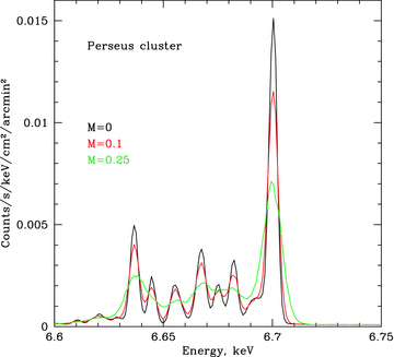
Simulated spectrum of the Perseus cluster core (central 130 kpc), calculated assuming different Mach numbers of the turbulence. At each point along the line of sight the locally emitted spectrum is calculated using Astrophysical Plasma Emission Code (APEC; Smith et al. 2001) model and using known radial density and temperature dependencies. The lines are then broadened by the thermal and turbulent motions using equation (24) (see Section 7.2) and the whole spectrum is projected along the line of sight. The case of pure thermal broadening of lines is shown in black. This plot shows that (i) turbulent broadening is important even for the modest level of turbulence and (ii) lines overlap with each other, especially if turbulent motions are present.

Open in new tabDownload slide

The presence of several closely spaced emission lines, modest level of turbulence (i.e. modest ratio of the turbulent and thermal broadenings), the lack of very strong stochastic density fluctuations on top of a regular radial structure, and often a strong level of Poisson noise affect the choice of the simplest viable approach to relate future observables and most basic characteristics of the ICM gas velocity field.

The fact that lines in spectra of galaxy clusters are very close to each other (e.g. Fig. 1) and the line ratio is temperature dependent can be circumvented by estimating the mean shift and broadening with direct fitting of the projected spectra with the plasma emission model (possible multi-temperature model). While the small thermal broadening of lines from heavy elements helps to extend the applicability of VCA/VCS techniques into the subsonic regime (see Esquivel et al. 2003; Lazarian & Esquivel 2003; Chepurnov et al. 2010), limited spectral resolution of the next generation of X-ray bolometers [e.g. full width at half-maximum (FWHM) ∼ 5 eV for Astro-H] reduces the measured inertial range in the velocity domain. Direct application of SCF and PCA methods to galaxy clusters can also be challenging, especially when the spectra are dominated by the Poisson noise. These problems should be alleviated with missions like ATHENA, having very large effective area and an energy resolution of ∼2.5 eV.

Below we suggest to use the simplest ‘centroids and broadening’ approach as a first step in studying the ICM turbulence. This approach assumes that at any given position one fits the observed spectrum with a model of an optically thin plasma (including all emission lines) and determines the velocity centroid and the line broadening. This reduces the whole complexity of X-ray spectra down to two numbers – shift and broadening. A simple analysis of existing hydrodynamic simulations of galaxy clusters shows that this approximation does a good (although not perfect) job in describing the profiles of emission lines (see e.g. fig. 2 in Inogamov & Sunyaev 2003). At the same time this approach is the most effective in reducing the Poison noise in the raw measured spectra. We show below that in spite of its simplicity this approach provided an easy way to characterize the most basic properties of the ICM velocity field.

Clearly, more sophisticated methods developed for the ISM turbulence (e.g. Lazarian 2009) will eventually be adopted to the specific characteristics of the ICM turbulence and X-ray spectra, potentially providing a more comprehensive description of the ICM turbulence, once the data of sufficient quality become available.

The structure of the paper is as follows. In Section 2 we describe and justify models and assumptions we use in our analysis. In Section 3 we specify observables which can be potentially measured and their relation to the 3D velocity power spectrum. Section 4 shows the relation between observed velocity dispersion and the SF of the velocity field. A way to constrain length scales (size of the energy-containing eddies) of motions using observed projected velocity is presented in Section 5. Method to recover 3D velocity power spectrum (PS) from 2D projected velocity field is discussed in Section 6. Discussion and conclusions are given in Sections 7 and 8, respectively.

2 BASIC ASSUMPTIONS AND MODELS

We consider a spherically symmetric galaxy cluster, which has a peaked X-ray emissivity profile. The electron number density is described by the β-model profile

1

where n₀ is the electron number density in the cluster centre (normalization) and r_c is the core radius. The β-model provides a reasonably good description of observed surface brightness (Cavaliere & Fusco-Femiano 1978) in the central regions of galaxy clusters. At large radii β-model is not a good description of surface brightness (see e.g. Vikhlinin et al. 2006). However, the simplicity of the model allows us to illustrate the method and make analytical calculations.

We have chosen β= 0.6 and r_c= 10 kpc for the demonstration of our analysis. Parameter β usually varies 0.4 < β < 1 for galaxy clusters (see e.g. Chen et al. 2007), herewith a large fraction of clusters have β∼ 0.6. r_c can vary from a few kpc to a few hundreds kpc. In order to better illustrate the main idea of the method, we considered cool-core clusters with small core radius r_c (it is necessary to have a gradient of surface brightness down to the smallest possible projected distances; see Section 4 for details).

We describe the line-of-sight component of the 3D velocity field as a Gaussian isotropic and homogeneous random field. This allows us to gauge whether useful statistics could in principle be obtained. However, there is no guarantee that this assumption applies to the velocity field in real clusters. For example, Esquivel et al. (2007) using numerical simulations have shown that in the case of supersonic turbulence in the ISM, the non-Gaussianity causes some of the statistical approaches (based on the assumption of Gaussianity) to fail. The same authors demonstrated that for the subsonic turbulence the Gaussianity assumption holds much better. This is encouraging since in clusters we expect mostly subsonic turbulence. Nevertheless, the methods discussed here require numerical testing using galaxy clusters from cosmological simulations. We defer these tests for future work.

PS of velocity field is described by a cored power-law model4

2

where k_m is a break wavenumber (in our simple model k_m characterizes the injection scale), α is a slope of the PS at k > k_m (inertial range) and B is the PS normalization, which is defined so that the characteristic amplitude A of velocity fluctuations at k=k_ref is fixed, i.e.

3

The cored power-law model of the PS is a convenient description of the PS for analytical calculations and at the same time resembles widely used broken power-law model.

Now let us specify the choice of parameters α and k_m in the model of the velocity PS. Cluster mergers, motions of galaxies and active galactic nuclei (AGN) feedback lead to turbulent motions with eddy sizes ranging from Mpc near the virial radius down to a few tens of kpc near the cluster core (see e.g. Sunyaev, Norman & Bryan 2003). For our analysis we vary injection scales from 20 kpc (k_m= 0.05 kpc⁻¹) to 2000 kpc (k_m= 0.0005 kpc⁻¹).

Parameter α– the slope of the PS – can be selected using standard arguments. If most of the kinetic energy is on large scales (injection scales), i.e. the characteristic velocity V decreases with k then the power spectrum with α≤−3. At the same time the turnover time of large eddies should not be larger than the turnover time of small eddies, i.e. t=l/V= 1/(kV) is a decreasing function of the wavenumber k. Therefore, V∝k^γ with γ≥−1 and with α≥−5. So we expect the slope of the PS to be in the range −5 ≤α≤−3. We will use α=−11/3 (slope of the Kolmogorov PS), α=−4 and α=−4.5.

3 OBSERVABLES AND 3D VELOCITY POWER SPECTRUM

Gas motions in relaxed galaxy clusters are predominantly subsonic, and to the first approximation the width and centroid shift of lines measured with X-ray observatories contain most essential information on the ICM velocity field (see e.g. Inogamov & Sunyaev 2003; Sunyaev et al. 2003). That is, we have information about:

• surface brightness in lines (Fig. 2, left-hand panel), i.e. if one assumes isothermal galaxy cluster (effects of non-constant temperature and abundance of elements are discussed in Section 6),

• emissivity-weighted projected velocity (Fig. 2, middle panel) (in practice measured projected velocity is averaged over some finite solid angle; see Section 5),

• emissivity-weighted velocity dispersion (Fig. 2, right panel) ⁠,

Figure 2

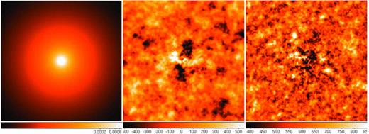
Maps of observables. Left: surface brightness in line (arbitrary units); middle: emissivity-weighted projected velocity field in km s⁻¹ (centroid shift of the line); right: velocity dispersion in km s⁻¹ (line broadening). Here, we consider only the velocity component along the line of sight. We assume β-model of the emissivity with β= 0.6 and r_c= 10 kpc and a random, uniform and homogeneous Gaussian velocity field with cored power-law 3D power spectrum (equation C1) with k_m= 0.005 kpc⁻¹ and Kolmogorov slope α=−11/3 (see Section 2). The size of each map is 1 × 1 Mpc.

Open in new tabDownload slide

 where n_e denotes the number electron density and V is a velocity component along the line of sight. Here 〈〉_z denotes emissivity-weighted averaging along the line of sight, which we assume to be along z direction.

Relation between the PS of the 3D velocity field, the 2D projected velocity and the velocity dispersion for a line of sight with projected coordinates (x, y) is as follows:

4

and

5

where 〈〉 is the ensemble averaging over a number of realizations, is an expectation value of the 2D PS of the observed projected velocity field V(x, y), P_3D is the PS of the 3D velocity field and P_EM is the PS of normalized emissivity distribution along the line of sight. For more details, see Appendixes A and B.

In Fig. 3 we illustrate equation (5) for a simple spherically symmetric β-model of galaxy cluster with core radius r_c= 10 kpc and β= 0.6. 3D velocity PS has a cored power-law model (equation 2), i.e. is flat on k < k_m= 0.005 kpc⁻¹ and has a Kolmogorov slope α=−11/3 on k > k_m. Observed velocity dispersion averaged over 100 realizations is shown with dots; the error bars show the expected uncertainty in one measurement. The right-hand side of equation (5) is shown in red. Minor difference between two curves at small R is due to finite resolution of simulations.

Figure 3

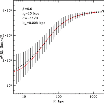
Expected dependence of the line-of-sight velocity dispersion (line width) on the projected distance R from the cluster centre. The increase in the effective length along the line of sight with the projected distance R implies that progressively large eddies contribute to the observed line broadening. We assume a β-model of the density distribution in an isothermal galaxy cluster (equation 1) and a cored 3D power-law model of the velocity power spectrum with slope α and break at k=k_m (equation 2). Parameters are shown on the top left corner of the plot. Black dots with error bars: velocity dispersion with uncertainties in a single realization, obtained by averaging over 100 realizations (the left part of equation 5), red curve: analytic expression of the velocity dispersion (the right-hand side of equation 5, see also Appendix B).

Open in new tabDownload slide

Once we construct the map of projected velocity V_2D(x, y), one can also find rms velocity of the 2D field at each distance r from the cluster centre as

6

where 〈V_2D(x, y)〉_r denotes mean velocity in ring at distance r from the centre. Below we use the observed velocity dispersion and rms of the projected velocity field to constrain the power spectrum.

4 STRUCTURE FUNCTION AND OBSERVED VELOCITY DISPERSION

Often a SF of the velocity field is used instead of the power spectrum, which is defined as

7

where averaging is over a number of pairs of points in space separated by distance Δx. The line-of-sight velocity dispersion can be linked to the SF. Indeed, since the emissivity peaks at the centre of the cluster and declines with the radius, the largest contribution to the total flux and to the line-of-sight velocity dispersion at distance R from the centre comes from the region, the size of which is ∝R.

The SF and the observed velocity dispersion can be related to the PS (see appendixes C and D):

8

and

9

where P_1D is an expectation value of the 1D velocity PS and P_EM is a PS of normalized emissivity along the line of sight. Fig. 4 shows the integrands in equations (8) and (9) multiplied by k and 2k, respectively, for the line of sight near the cluster centre (black curves) and at a projected distance R= 800 kpc from the centre (red curves). Extra factor of 2 for σ²(R) is introduced to compensate for the factor of 2 in front of the expression (8) for the SF. It is more clear if one considers the limits of these equations at large x and R. When x→∞ then oscillates with high frequency over relevant interval of k and mean value of is ∼1. When R→∞ the emissivity distribution is very broad and P_EM is almost a δ-function. Therefore,

10

and

11

From Fig. 4, it is clear that the integrands in equations (8) and (9) are very similar, suggesting that observed 2σ²(R) should correlate well with the SF.

Figure 4

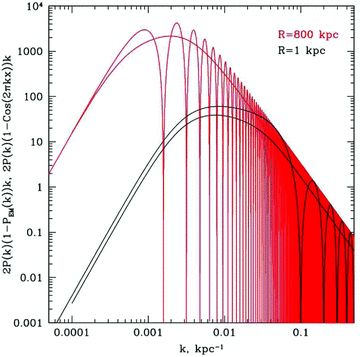
Integrand from equation (8) multiplied by k (oscillating function) and integrand from equation (9) multiplied by 2k (non-oscillating function) calculated for projected distance R= 1 kpc (black curves) and R= 800 kpc from the centre (red curves). The scales where these functions have maxima provide dominant contribution to the line-of-sight velocity dispersion and SF. The shift of the dominant scale to smaller k at large projected distances shows that different parts of the power spectra are probed with σ²(R) measured at different R. The shift of the dominant scale in the SF (l_eff(R)) traces the similar shift for σ²(R). This suggests that σ²(R) measurements can be used as a proxy for the SF at a range of scales.

Open in new tabDownload slide

The SF and the velocity dispersion (equations C5 and D1, respectively) are plotted in Fig. 6 in left-hand panel. We fixed parameters of the β-model of the cluster and varied the slope α and break k_m of the power spectrum model (equation 2). The relation of SF and 2σ² is shown in the left-bottom panel in Fig. 6. For a given R, 2σ²(R) is used for x-axis, while the SF is plotted as a function of l_eff(R), where l_eff is an effective length along the line of sight, which provides dominant contribution to the line flux. l_eff is found from the condition that

12

Relation between l_eff and projected distance depends on the β-model of galaxy cluster as shown in Fig. 5.

Figure 6

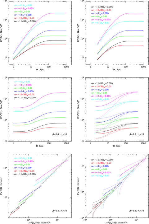
Left-hand panel: SF (see analytical expression C5), line-of-sight velocity dispersion multiplied by a factor of 2 (equations D1 and D5) and their relation for different models of cored power-law power spectrum (equation C1). Parameters of the power spectrum (slope and break wavenumber) are shown in the top left corner. Parameters of the β-model are given in the bottom right corner. Right-hand panel: the same as left-hand panel, but calculated by averaging over 100 statistical realizations of velocity field. The uncertainties in single measurement of the velocity dispersion are shown with dotted curves. The choice of parameters is discussed in Section 2.

Open in new tabDownload slide

Figure 5

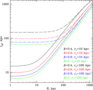
Dependence of the effective length along the line of sight l_eff(R) (equation 12) on the projected distance R for different β-models of galaxy clusters.

Open in new tabDownload slide

We then made multiple statistical realizations of the PS for a simple β-model of galaxy cluster with β= 0.6 and r_c= 10 kpc to estimate the uncertainties. The size of the box is 1 Mpc³ and resolution is 2 kpc. We assume that the 3D PS of the velocity field has a cored power-law model (equation C1) with slope α and break wavenumber (injection scale) at k_m. We made 100 realizations of a Gaussian field with random phases and Gaussian-distributed amplitudes in Fourier space. Taking inverse Fourier transform, we calculated one component of the 3D velocity field (component along the line of sight) in the cluster. SF and the line-of-sight velocity dispersion are evaluated using resulting velocity field. Right-hand panel in Fig. 6 shows velocity dispersion along the line of sight and SF averaged over 100 realizations. The expected uncertainty in single measurement of the velocity dispersion is shown with dotted curves. One can see that the overall shape and normalization of SF and 2σ² are the same as predicted from analytical expressions (left-hand panel in Fig. 6); however, there are minor differences (especially at small R) due to limited resolution of simulations. Relation between 2σ² and SF is in good agreement with expectation relation; however the uncertainty in measured velocity dispersion (due to the stochastic nature of the velocity field) is significant (see Section 6).

5 LENGTH SCALES OF MOTIONS AND OBSERVED rms VELOCITY OF PROJECTED VELOCITY FIELD

Let us now consider rms of the projected velocity field. During observations one gets spectra from a region, minimum size of which is set by angular resolution and/or the sensitivity of the instrument. rms velocity at certain position (x,y) for random realizations of the velocity field is defined as (see Appendix E)

13

where P_SH(k_x, k_y) is a PS of a mask, where the mask is defined as zero outside and unity inside the region, from which the spectrum is extracted (see Appendix E for details). Velocity dispersion (i.e. the line broadening) measured from the same region is

14

Therefore the ratio is

15

which can be used as an additional proxy of the length scales of gas motions. This ratio is mostly sensitive to the break of the cored power-law model of the PS k_m. Basically at a given line of sight, which is characterized by an effective length l_eff the small-scale motions (i.e. k > 1/l_eff) are mostly contributing to line broadening, while larger scale motions predominantly contribute to the rms of the projected velocity field.

Fig. 7 shows the ratio and its uncertainty calculated for different values of parameter k_m. V_rms and σ are averaged over rings at distance R from the cluster centre. Clearly, if k_m is large, then all motions are on small scales and the ratio is small. The larger is the k_m, the more power is at large scales and the larger is the V_rms. The larger is the injection scale, the stronger is the increase of the ratio with distance and the more prominent is the peak (see Fig. 7). Here we assume that the full map of projected velocity field is available. Clearly, the uncertainties will increase if the data are available for several lines of sight, rather than for the full map.

Figure 7

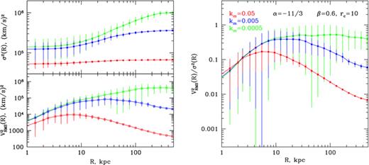
Velocity dispersion and V_rms as functions of distance from the cluster centre with uncertainties due to the stochastic nature of the velocity field (left panels) and their ratio from equation (15) (right-hand panel). V_rms(R) and σ(R) are averaged over a ring at distance R from the cluster centre. Errors show the characteristic uncertainties in one measurement. The slope of assumed velocity PS is −11/3. Break wavenumber k_m of the PS is shown on the right-hand panel. Colour coding is the same in both panels.

Open in new tabDownload slide

Looking at equation (15) it is easy to predict the behaviour of the ratio on small and large projected distances R. Let us specify the shape of area, namely assume that we measure velocity in circles with radius R around the cluster centre. When R→ 0 then the region is very small and P_SH(k_x, k_y) → 1 over broad range of wavenumbers k < 1/R and the ratio ⁠. At large RP_SH(k_x, k_y) → 0 and P_EM(k_z) → 0 [since distribution along the line of sight on large R is broad], equation (15) becomes

16

and it is a decreasing function of R.

The sensitivity of ratio to the slope of the power spectrum is modest. There are only changes in normalization, but the overall shape is the same.

6 RECOVERING 3D VELOCITY POWER SPECTRUM FROM 2D PROJECTED VELOCITY FIELD

Mapping of the projected velocity field V_2D(x, y) provides the most direct way of estimating the 3D velocity field PS. The 2D and 3D PS are related according to equation (4), which we re-write as

17

where ⁠. This equation can be written as

18

The contribution of the second term to the integral is small since P_EM(k_z, x, y) → 0 on k > 1/l_eff. In the limit of k≫ 1/l_eff (at a given projected distance) the expression reduces to

19

i.e. 2D PS is essentially equal to the 3D PS of the velocity field apart from the normalization constant ∫P_EM(k_z, x, y)dk_z, which is easily measured for a cluster. We show below that this simple relation (19) provides an excellent approximation for full expression (17) for a Coma-like clusters with flat surface brightness core. For peaked clusters (cool core) P_3D/P_2D depends on projected distance from the cluster centre since l_eff changes significantly with distance.

It is convenient to use characteristic scale-dependent amplitudes of the velocity field variations, rather than the PS. The amplitude for 3D and 2D spectra is defined as

20

21

In these notations the relation (19) between PS transforms to

22

Integral ∫P_EM(k_z, x, y) dk_z can be estimated as ⁠, since the largest contribution is on k < 1/l_eff. Equation (22) becomes

23

The essence of this relation is that the amplitude of the 3D velocity fluctuations is attenuated in the 2D projected velocity field by a factor of order ⁠, where N_edd is the number of independent eddies which fit into effective length along the line of sight.

We illustrate the above relation for the case of the Coma cluster. The density distribution in the Coma can be characterized by a β-model with β= 0.6 and co-radius r_c= 245 kpc. In Fig. 8 we plot the ratio A_3D(k)/A_2D(k) evaluated using equations (19) and (17) for a number of 3D PS models calculated at two projected distances from the Coma centre. One can see that on spatial scales of less than 1 Mpc, equation (22) is fully sufficient. The variations of the relation for different projection distances (projected distances from 0 to 300 kpc were used) affect only the normalization of the relation and can easily be accounted for.

Figure 8

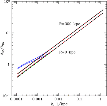
The ratio of 3D and 2D amplitudes as a function of k (equation 17) for a β-model cluster with β= 0.6 and r_c= 245 kpc (Coma-like cluster). A cored power-law model is used for the 3D power spectrum, according to equation (2). Two projected distances R were used: R= 0 and 300 kpc. Solid lines with different colours correspond to different break wavenumbers in the 3D power spectrum: k_m= 3 × 10⁻⁴, 3 × 10⁻³, 3 × 10⁻² kpc⁻¹ and different slopes of the spectrum α= 3.5, 4.0, 4.5. For a given projected distance the curves, corresponding to different power spectra model, lay on top of each other, independently of the slope of the power spectrum, except for the case with very low break wavenumber k_m= 3 × 10⁻⁴ (blue curves). For comparison, the thick dashed lines show the ratio, calculated using simplified equation (19). Clearly, in the range of scales from Mpc and below the simple relation between 3D and 2D amplitudes is fully sufficient to convert the observed 2D power spectrum into the power spectrum of the 3D velocity field, unless the break of the power spectrum is at very large scales of few Mpc.

Open in new tabDownload slide

With Astro-H the 2D velocity field in the Coma can be mapped with the ∼1.7 arcmin resolution, which corresponds to ∼46 kpc. Mapping 450 × 450 kpc central region of the Coma would require about 36 pointings. For practical reasons it may be more feasible to make a sparse map (e.g. two perpendicular stripes) to evaluate A_2D (e.g. computing correlation function or using a method described in Arévalo et al. 2012).

7 DISCUSSION

7.1 Limiting cases of small- and large-scale motions

Measuring characteristic amplitude of mean velocity (V_rms) and velocity dispersion (σ) we can distinguish whether the turbulence is dominated by small- or large-scale motions. Clearly, the motions on scales much smaller than the effective length along the line of sight near the cluster centre can only contribute to the line broadening. This sets the characteristic value of the lowest spatial scale which can be measured. The largest measurable scale is set by the maximum distance R_max from the cluster centre where the line parameters can be accurately measured without prohibitively long exposure time. Thus, the range of scales l, which can be probed with these measurements, is l_eff(R= 0) < l < R_max. The crucial issue in the measurements is ‘sample variance’ of measured quantities caused by the stochastic nature of turbulence. We can expect two limiting cases (see Fig. 7).

(1) Small-scale motions

In case of small-scale motions l≪l_eff(R= 0) [i.e. k_m≫l_eff(R=0)] one expects σ(R) to be independent of radius and V_rms(R) ≪σ(R). σ(R) is expected to have low sample variance and can be measured accurately even for a single line of sight, provided sufficient exposure time. Measurements of V_rms(R) are strongly affected by sample variance and depend on the geometry of the measured map of the projected velocity dispersion V(x, y). If V(x, y) is measured only at two positions, then the uncertainty in V_rms(R) is of the order of its value and the ratio σ(R)/V_rms(R) gives only low limit on k_m. We note that in this limit of small-scale motions the assumption of a uniform and homogeneous Gaussian field can be relaxed and measured values of line broadening σ simply reflect the total variance of the velocity along the given line of sight, while the possibility of determining the spatial scales of motions are limited. Variations of σ with radius will simply reflect the change of the characteristic velocity amplitude.

(2) Large-scale motions

In case if most of turbulent energy is associated with large scales [i.e. k_m≪l_eff(R= 0)], σ(R) is expected to increase with R and V_rms(R) ∼σ(R). In this case sample variance affects both σ(R) and V_rms(R). Mapping the whole area (as opposed to measurements at a few positions) would help to reduce the sample variance. Knowing the shape of σ(R) and estimates of k_m from σ(R)/V_rms(R) we can constrain the slope of power spectrum.

7.2 Effect of thermal broadening

Measuring velocity dispersion one should account for line broadening due to thermal motions of ions. Thermal broadening should be subtracted from measured width of line. The broadening of the line ⁠, where σ is measured Gaussian width of the line, is defined as

24

where σ_turb is the width due to turbulent motions and is the thermal broadening for ions with atomic weight A. The FHWM of the corresponding line is ⁠. Observed emission lines in the X-ray spectra of galaxy clusters correspond to heavy elements such as Fe, Ca, S. Because of a large value of A the contribution of thermal broadening is small even for modest amplitudes of turbulent velocities. Indeed, the atomic weight for iron is 56 and the thermal width of the iron line is ΔE∼ 3 eV (FWHM ∼ 5 eV) if one assumes the typical temperature of clusters ∼5 keV. At the same time, the gas motion with the sound speed would cause the shift of the line energy by ∼40 eV. As an example, we calculated the expected broadening of the He-like iron line at 6.7 keV for the Perseus cluster, assuming Kolmogorov-like PS of the velocity field with k_m= 0.001 kpc⁻¹ and varying total rms of the velocity field in one dimension. The model of the Perseus cluster was taken from Churazov et al. (2004) and modified at large distances according to Suzaku observations at the edge of the cluster (Simionescu et al. 2011), i.e. the electron number density is

25

and the temperature profile is

26

We assume that the abundance of heavy elements is constant and is equal to 0.5 relative to solar (Anders & Grevesse 1989). Fig. 9 shows the calculated width of 6.7 keV line assuming various 1D rms velocities. Thermal broadening is shown with the dashed magenta curve. One can see that thermal broadening starts to dominate broadening due to motions only if V_rms < 150 km s⁻¹. However, the lack of resonant scattering signatures in the spectrum of the Perseus cluster suggests that the expected velocity is higher than 400 km s⁻¹ in the centre of the Perseus cluster (Churazov et al. 2004). Astro-H will have energy resolution of 7 eV at 6.7 keV, therefore broadening due to gas motions with V_rms∝ 400 km s⁻¹ will be easy to observe (Fig. 9) in the Perseus cluster.

Figure 9

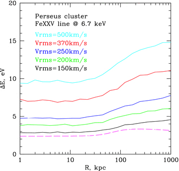
Width of the line of He-like iron line at 6.7 keV in Perseus cluster, assuming different 1D rms velocities. FWHM is related with the width as FWHM= 1.66ΔE. Solid curves show broadening due to gas motions only; the dashed curve shows the thermal broadening. Here we assumed the cored power-law 3D power spectrum with α=−11/3 and k_m= 0.001 kpc⁻¹.

Open in new tabDownload slide

7.3 The effect of radial variations of the gas temperature and metallicity

The analysis described in the previous sections was done assuming an isothermal β-model spherically symmetric cluster with emissivity simply ⁠. Clearly, real clusters are more complicated, even if we keep the assumption of spherical symmetry. First of all the gas temperature and metallicity often vary with radius. These variations will be reflected in the weighting function ⁠, which relates 3D velocity field and observables. To verify how strongly these assumptions affect the results, we calculated velocity dispersion assuming detailed model of the Perseus cluster (see above). We assumed constant abundance profile and more realistic peaked abundance profile, taken from Suzaku (Simionescu et al. 2011) and Chandra/XMM observations

27

We calculated the emissivity of the He-like iron line at 6.7 keV and used this emissivity as a weighting function for the calculation of the expected projected velocity and velocity dispersion. Fig. 10 shows the velocity dispersion along one line of sight calculated for the most simple model of emissivity and assuming more complicated models described above. One can see that mean value and uncertainties are very similar in all cases. Clearly that averaging velocity dispersion over a ring will decrease the uncertainty in one measurement (Fig. 10, black dashed curve).

Figure 10

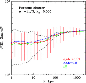
Velocity dispersion in the Perseus cluster as a function of distance from the centre for different emissivity and abundance profiles. Parameters of assumed velocity PS are shown in the top left corner. Green: simple approximation of emissivity ⁠; blue: emissivity at 6.7 keV line and flat abundance; red: emissivity at 6.7 keV line and peaked abundance (equation 27) in the centre (see text for details). Black dashed curve shows expected uncertainty in measurements of velocity dispersion observed in a ring.

Open in new tabDownload slide

7.4 Influence of density fluctuations

The hot gas density in galaxy clusters is strongly peaked towards the centre. However, besides the main trend, there are density fluctuations, which could contribute to the observed fluctuations of the projected velocity. Let us split the density field in two components

28

where n₀ corresponds to the smooth global profile and δn represents fluctuating part. Neglecting terms of the order (δn)², the emissivity-weighted projected velocity is

29

The analysis of X-ray surface brightness fluctuations in the Coma cluster (e.g. Churazov et al. 2012) has shown that the amplitude of the density fluctuations is of the order of ∼2–10 per cent. Assuming that the same number is applicable to other clusters, the second term in equation (29) is small and the contribution of the density fluctuation to projected velocity can be neglected.

7.5 Measurement requirements

To illustrate the most basic requirements for the instruments to measure the ICM velocity field, let us consider two examples of a rich cluster and an individual elliptical galaxy, representing the low temperature end of the cluster-group-galaxy sequence:

• Perseus cluster, T_mean= 5 keV, line of Fe xxv at 6.7 keV, distance 72 Mpc.

• Elliptical galaxy NGC 5813, T_mean= 0.65 keV, line of O viii at 0.654 keV, distance 32.2 Mpc.

Table 1 shows the FWHM of these lines calculated if only thermal broadening is taken into account, shift of the line energy in the case of gas motions with V=c_s and desirable angular resolution of the instrument. Future X-ray missions, such as Astro-H and ATHENA, will have energy resolution ∼5 eV and ∼3 eV, respectively. Such energy resolution is sufficient to measure broadening of lines in hot systems like galaxy clusters. Cold systems, like elliptical galaxies, require even better energy resolution. However, turbulence can still be measures using the resonant scattering effect (see e.g. Werner et al. 2009; Zhuravleva et al. 2011) or by using grating spectrometer observations. Angular resolution of ∼1 arcmin for nearby galaxy clusters should be sufficient to study the most basic characteristics of the ICM velocity field, while for elliptical galaxies the resolution at the level of ∼ arcsec (comparable with Chandra resolution) would be needed.

Astro-H observatory will have energy resolution ∼5 eV, field of view 2.85 arcmin and angular resolution 1.7 arcmin, which means that it will be possible to measure shift and broadening of lines as a function of projected distance from the centre in nearby clusters. For example if one assumes that rms velocity of gas motions in Perseus cluster is ∼300 km s⁻¹, then ∼4 × 10⁵ s is enough to measure profiles of mean velocity and velocity dispersion with a statistical uncertainty of ∼30 km s⁻¹ (90 per cent confidence) in a stripe ±200 kpc (seven independent pointing and 28 independent measurements in 1.4 × 1.4 arcmin² pixels) centred in the centre of the cluster.5 In order to measure velocity with the same accuracy at larger distances from the centre, e.g. at 500 kpc and 1 Mpc, one would need 8 × 10⁵ s and 4 × 10⁶ s exposure, respectively.

8 CONCLUSIONS

Various methods of constraining the velocity power spectrum through the observed shift of line centroid and line broadening are discussed.

• Changes of the line broadening with projected distance reflect the increase of the spread in the velocities with distance, closely resembling the behaviour of the SF of the velocity field.

• Another useful quantity is the ratio of the characteristic amplitude of the projected velocity field to the line broadening. Since the projected velocity field mainly depends on large-scale motions, while the line broadening is more sensitive to small-scale motions, this ratio is useful diagnostics of the shape of the 3D velocity field power spectrum.

• Projected 2D velocity field power spectrum can be easily converted into 3D power spectrum. This conversion is especially simple for cluster with an extended flat core in the surface brightness (like Coma cluster).

Analytical expressions are derived for a β-model clusters, assuming homogeneous isotropic Gaussian 3D velocity field. The importance of the sample variance, caused by the stochastic nature of the turbulence, for the observables is emphasized.

IZ, EC and AK would like to thank Kavli Institute for Theoretical Physics (KITP) in Santa Barbara for hospitality during workshop ‘Galaxy clusters: crossroads of astrophysics and cosmology’ in 2011 March–April, where part of the work presented here was carried out. This research was supported in part by the National Science Foundation under Grant No. NSF PHY05-51164 and by the Division of Physical Sciences of the RAS (the program “Extended objects in the Universe”, OFN-16). IZ would like to thank the International Max Planck Research School on Astrophysics (IMPRS) in Garching.

Footnotes

REFERENCES

Appendices

APPENDIX A: 3D VELOCITY POWER SPECTRUM AND PROJECTED VELOCITY FIELD

Let us assume that the line-of-sight component of the 3D velocity field V_3D(x, y, z) is described by a Gaussian (isotropic and homogeneous) random field. We assume that the centroid shift and the width of lines contain most essential information on the velocity field. Here and below we adopt the relation k= 1/r without factor (see Section 2 for details).

Projected 2D velocity along the line of sight (observed centroid shift of the emission line) in z direction is

(A1)

where V_3D is the z component of the 3D velocity field and n_e is the electron number density. Denoting normalized emissivity along the line of sight at a certain position with coordinates (x,y) as the previous relation can be re-written as

(A2)

Applying the convolution theorem one can find the Fourier transform of V_3D(x, y, z)ε(z) as

(A3)

where and are Fourier transforms of the 3D velocity field and normalized emissivity, respectively. The projection-slice theorem states that

(A4)

Accounting for (A3) and (A4) we can write the Fourier transform of 2D velocity field as

(A5)

where * denotes conjugation.

Averaging over a number of realization we find the power spectrum of the projected mean velocity

(A6)

The right part of the equation above can be re-written as

(A7)

Since phases are random, all cross terms after averaging over a number of realizations will give 0 if ⁠. Therefore,

(A8)

Denoting power spectra of the 3D velocity field and normalized emissivity as P_3D and P_EM, respectively, the final expression is

(A9)

APPENDIX B: 3D VELOCITY POWER SPECTRUM AND PROJECTED VELOCITY DISPERSION

Projected mean velocity dispersion for the line of sight with coordinates (x,y) averaged over a number of realization is defined as

(B1)

It can be re-written as

(B2)

Expanding V_3D and V_2D through the Fourier series, averaging over realizations and keeping non-zero cross terms will give

(B3)

Since emissivity along the line of sight is normalized so that and accounting for equation (A9) the final expression for projected velocity dispersion will be

(B4)

APPENDIX C: RELATION BETWEEN STRUCTURE FUNCTION AND CORED POWER-LAW 3D POWER SPECTRUM

Let us assume 3D isotropic and homogeneous PS of the velocity field is described as

(C1)

where k_m is a wavenumber at which β-model has a break (e.g. an injection scale in turbulence model), α is a slope of PS on k > k_m and B is PS normalization, which is defined so that the characteristic amplitude A of velocity fluctuations at k_ref is fixed, i.e.

(C2)

Integrating C1 over ⁠, one can find 1D PS

(C3)

SF is related to 1D PS by the transformation (Rytov, Kravtsov & Tatarskii 1988)

(C4)

Substituting (C3) with (C4) and assuming α > 3 yield

(C5)

where and K_α is a modified Bessel function of the second kind.

APPENDIX D: RELATION BETWEEN VELOCITY DISPERSION ALONG THE LINE OF SIGHT AND POWER SPECTRUM

P_1D and P_3D are related as ⁠, therefore equation (B4) can be re-written as

(D1)

where R is projected distance from the centre.

If electron number density is described by β-model with normalization n₀ and core radius R_c

(D2)

then the emissivity is

(D3)

where r²=R²+z², and we assume normalization n₀= 1. The Fourier transform of emissivity is

(D4)

where terms with are zero since integrand is symmetrical. Dividing (D4) by the total flux and assuming β > 1/6 one can find weight W(k_z) as

(D5)

where and K_α is a modified Bessel function of the second kind.

APPENDIX E: RATIO OF OBSERVED rms VELOCITY TO OBSERVED VELOCITY DISPERSION

Let us assume that spectrum is extracted from the region with the area ∫_shapedx dy. The rms velocity from this spectrum averaged over a number of realizations is

(E1)

where 〈〉 denotes averaging over realizations. Accounting for equation (A2) we can re-write the first term in the above equation as

(E2)

where F_EM is a Fourier transform of emissivity along the line of sight. Averaging over a number of realizations will leave non-zero terms only if k₁=k₂. Therefore, the first term in equation (E1) is

(E3)

The second term in equation (E1) can be written as

(E4)

Squaring and averaging over realizations yield

(E5)

or

(E6)

where S(x, y) is a mask, which is zero outside and unity inside the area, from which spectrum is extracted. Denoting power spectrum of S(x, y)/(∫_shapedxdy)² as P_SH(k_x, k_y), the second term in equation (E1) becomes

(E7)

Therefore, the final expression for the rms of the projected velocity field is

(E8)

Moreover. the ratio of and velocity dispersion along the line of sight is

(E9)