Mass ratio from Doppler beaming and Rømer delay versus ellipsoidal modulation in the Kepler data of KOI-74*

Abstract

1 INTRODUCTION

The primary science goal of the Kepler mission is the detection of Earth-like exoplanets, but its highly accurate photometric observations also reveal hundreds of eclipsing binary stars (Slawson et al. 2011) and are well suited for the study of stellar variability at unprecedentedly low amplitudes (Debosscher et al. 2011). In this paper, we present an analysis of 212 d of Kepler data of the eclipsing binary KOI-74 (KIC 6889235) and spectra taken at different orbital phases.

The system consists of a main-sequence A star primary and a less massive companion. Its light curve shows deeper eclipses than transits,1 which implies that the companion is hotter than the primary. There is a clear asymmetric ellipsoidal modulation pattern in which the flux maximum after the transits is larger than the maximum after the eclipses. Rowe et al. (2010) suggested that the asymmetry in the ellipsoidal modulation is due to a star spot. van Kerkwijk et al. (2010) instead attributed it to Doppler beaming. This effect is caused by the stars’ radial velocities which shift the spectrum, modulate the photon emission rate and beam the photons somewhat in the direction of motion. The effect was, as far as we are aware, first discussed in Shakura & Postnov (1987) and first observed by Maxted, Marsh & North (2000). Its expected detection in Kepler light curves was suggested and discussed by Loeb & Gaudi (2003) and Zucker, Mazeh & Alexander (2007). The detection of Doppler beaming in Kepler light curves has led to the discovery of several non-eclipsing short-period binary systems (Faigler et al. 2012) and it has been shown that it can also be observed in planetary systems (see e.g. Mazeh & Faigler 2010; Shporer et al. 2011). Bloemen et al. (2011) detected Doppler beaming in the Kepler light curve of KPD 1946+4340 and presented the first comparison between a radial velocity amplitude derived from Doppler beaming with a spectroscopic value. In the case of KPD 1946+4340, the results were found to be consistent. For KOI-74, spectroscopic radial velocity measurements were recently presented by Ehrenreich et al. (2011). In this paper, we present independent spectroscopic radial velocity measurements which we compare with the photometric radial velocity amplitude prediction.

Earlier analyses of the Kepler light curve of KOI-74 are presented in Rowe et al. (2010) and van Kerkwijk et al. (2010). Rowe et al. (2010) measured the mass ratio of the system from the amplitude of the ellipsoidal modulation and found a companion mass of 0.02–0.11 M_⊙. van Kerkwijk et al. (2010) built on these results (e.g. they used the inclination value reported by Rowe et al. 2010) but claimed that the mass ratio of the system could not be determined reliably from the ellipsoidal modulation amplitude. Instead, they used the radial velocity information from the Doppler beaming signal to derive a companion mass of 0.22 ± 0.03 M_⊙. They concluded that the companion has to be a low-mass white dwarf and showed that the system properties are in good agreement with a binary that has undergone a phase of stable Roche lobe overflow from the more massive star to the less massive star. This puts KOI-74 in an evolutionary stage that follows on that of systems such as WASP J0247−2515, which Maxted et al. (2011) recently identified as a binary consisting of an A-star and a red giant core stripped from its envelope. Up to now, four close binaries consisting of a white dwarf and a main-sequence star of spectral type A or F have been found in Kepler data (Rowe et al. 2010; van Kerkwijk et al. 2010; Breton et al. 2012; Carter, Rappaport & Fabrycky 2011).

We remodel the Kepler light curve of KOI-74, adding an additional 175 d of data compared to the previous studies and perform Markov chain Monte Carlo (MCMC) simulations to explore the uncertainty on the derived system parameters. We will revisit the issue of the true mass ratio of the system, using input from the light-curve analysis (Doppler beaming, ellipsoidal modulation and Rømer delay) and spectroscopy.

2 SPECTROSCOPY

To determine the spectral type, the rotational velocity and the radial velocity amplitude of the primary, we obtained 46 high-resolution (R∼ 85 000) échelle spectra using the HERMES spectrograph (Raskin et al. 2011) at the 1.2-m Mercator telescope (La Palma, Canary Islands). These were reduced using the standard instrument-specific data reduction pipeline. Additionally, we obtained 29 spectra with the ISIS spectrograph mounted on the 4.2-m William Herschel Telescope (La Palma, Canary Islands). We averaged the HERMES spectra, after shifting out the primary’s radial velocity. From the average spectrum, we measured the rotational velocity of the primary vsin i= 164 ± 9 km s⁻¹, using the Fourier method presented in Gray (1992), from the Mg iiλ4481 line. Compared to other techniques such as fitting broadened synthetic spectra, the Fourier method has the advantage of being rather insensitive to other line-broadening mechanisms (see e.g. Simón-Díaz & Herrero 2007). The Mg iiλ4481 line is a doublet with components at 4481.126  and 4481.325 Å, which leads to an overestimation of vsin i (see e.g. Royer et al. 2002). By applying the same method to a synthetic spectrum with a comparable rotational broadening, we find that we can expect our vsin i measurement to be overestimated by about 10 km s⁻¹ due to the double nature of the line. Given this overestimation, our result is in line with the values mentioned in the Note in proof of van Kerkwijk et al. (2010), 150 km s⁻¹, and in Ehrenreich et al. (2011), 145 ± 5 km s⁻¹. If the primary were in corotation with the binary orbit, we would expect vsin i∼ 25 km s⁻¹. The rotational velocity measured from spectroscopy thus implies that the primary is not in corotation but is instead a fast rotator. We have adopted vsin i= 150 ± 10 km s⁻¹ for the analysis presented in this paper. We also performed a spectral fit to the Balmer lines and Mg iiλ4481 using the solar metallicity synthetic spectra of Munari et al. (2005) and assuming a rotational velocity of 150 km s⁻¹. The fits to the spectral lines are shown in Fig. 1. The small emission feature in the core of the Hα and Hβ lines does not originate from any of the two binary components but is caused by sky emission (see also Ehrenreich et al. 2011). It is absent in the ISIS spectra, for which we could perform a background subtraction during the data reduction. We find that the primary has a gravity of log g∼ 4.27 and an effective temperature of T_eff∼ 9500 K. These results are in agreement with the spectral type A1V and T_eff= 9 400 ± 150 K derived by Rowe et al. (2010), from which they inferred a primary mass of M₁= 2.2 ± 0.2 M_⊙. We adopted T_eff= 9 500 ± 250 K for our analysis.

Figure 1

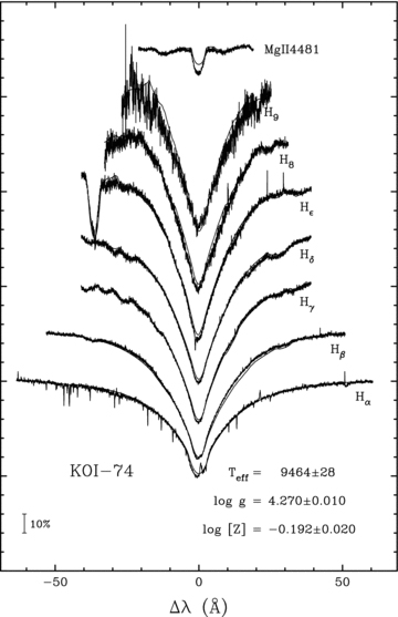
Fit to the spectral lines of KOI-74 using the average HERMES spectrum (after shifting the spectra to the rest frame of the primary) and the solar metallicity synthetic spectra of Munari et al. (2005). The uncertainties on the parameters indicated in the figure only reflect the formal errors on the fit.

Open in new tabDownload slide

We have used two techniques to derive the radial velocity amplitude of the A-star. The only metal line that is clearly detected in both the HERMES and ISIS spectra is the Mg ii line at 4481 Å. We measured the radial velocities from that line by fitting a Gaussian profile to it. We also measured the radial velocities from the Balmer lines at 4102, 4340 and 4861 Å simultaneously, by first normalizing the spectra using low-order splines (as described in Pápics et al. 2012), and then fitting a Gaussian to the core of the mean profile obtained by least-squares deconvolution (Donati et al. 1997). The measured radial velocity amplitudes and systemic velocities, assuming a circular orbit, are given in Table 1. The uncertainties on individual data points have been scaled to deliver a unit χ² per degree of freedom. The initial χ², before rescaling the uncertainties, is given in the table. The radial velocities measured from the Balmer lines are shown in Fig. 2, folded on the orbital period using the Kepler ephemeris as given in Rowe et al. (2010). Some spectra were taken in bad seeing conditions, which is reflected by the large error bars on a few of the data points. We have adopted the weighted mean velocity amplitude of our measurements, K₁= 15.4 ± 0.3 km s⁻¹, for the analysis presented in this paper. The weighted mean systemic velocity is γ= 49.1 ± 0.2 km s⁻¹. Our radial velocity amplitudes are in agreement with (but slightly lower than) the Ehrenreich et al. (2011) result of 18.2 ± 1.7 km s⁻¹. We provide the radial velocities we have measured from our spectra in electronic form with this paper (see Supporting Information).

Table 1

Open in new tab

Radial velocity amplitudes (K₁) and systemic velocities (γ) of KOI-74, measured from ISIS/WHT and HERMES/Mercator spectra. The uncertainties that are given are scaled to get a unit χ² per degree of freedom. Initial reduced χ² is given in the last column. Two techniques have been used: a Gaussian fit to the Mg ii line at 4481 Å and a Gaussian fit to the mean profile of the Balmer lines at 4102, 4340 and 4861 Å (see text for details).

Instrument	Lines	K1 (km s−1)	γ (km s−1)
ISIS	Balmer	15.8 ± 0.4	−50.9 ± 0.3	1.2
	Mg ii	15.4 ± 0.7	−49.3 ± 0.5	1.6
HERMES	Balmer	14.9 ± 0.4	−47.1 ± 0.3	0.5
	Mg ii	16.5 ± 1.3	−51.0 ± 1.0	2.3
Weighted mean (adopted)		15.4 ± 0.3	−49.1 ± 0.2

Instrument	Lines	K1 (km s−1)	γ (km s−1)
ISIS	Balmer	15.8 ± 0.4	−50.9 ± 0.3	1.2
	Mg ii	15.4 ± 0.7	−49.3 ± 0.5	1.6
HERMES	Balmer	14.9 ± 0.4	−47.1 ± 0.3	0.5
	Mg ii	16.5 ± 1.3	−51.0 ± 1.0	2.3
Weighted mean (adopted)		15.4 ± 0.3	−49.1 ± 0.2

Table 1

Open in new tab

Radial velocity amplitudes (K₁) and systemic velocities (γ) of KOI-74, measured from ISIS/WHT and HERMES/Mercator spectra. The uncertainties that are given are scaled to get a unit χ² per degree of freedom. Initial reduced χ² is given in the last column. Two techniques have been used: a Gaussian fit to the Mg ii line at 4481 Å and a Gaussian fit to the mean profile of the Balmer lines at 4102, 4340 and 4861 Å (see text for details).

Instrument	Lines	K1 (km s−1)	γ (km s−1)
ISIS	Balmer	15.8 ± 0.4	−50.9 ± 0.3	1.2
	Mg ii	15.4 ± 0.7	−49.3 ± 0.5	1.6
HERMES	Balmer	14.9 ± 0.4	−47.1 ± 0.3	0.5
	Mg ii	16.5 ± 1.3	−51.0 ± 1.0	2.3
Weighted mean (adopted)		15.4 ± 0.3	−49.1 ± 0.2

Instrument	Lines	K1 (km s−1)	γ (km s−1)
ISIS	Balmer	15.8 ± 0.4	−50.9 ± 0.3	1.2
	Mg ii	15.4 ± 0.7	−49.3 ± 0.5	1.6
HERMES	Balmer	14.9 ± 0.4	−47.1 ± 0.3	0.5
	Mg ii	16.5 ± 1.3	−51.0 ± 1.0	2.3
Weighted mean (adopted)		15.4 ± 0.3	−49.1 ± 0.2

Figure 2

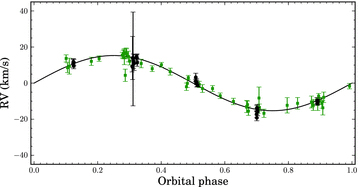
Radial velocity curve of the primary of KOI-74, measured by fitting a Gaussian profile to the mean profile of three Balmer lines (see text for details). The radial velocity measurements from ISIS/WHT spectra are represented by black circles, the measurements from HERMES/Mercator spectra by green squares, folded on the orbital period. The systemic velocity derived from both data sets has been subtracted. The error bars are scaled to deliver a unit χ² per degree of freedom.

Open in new tabDownload slide

3 KEPLER PHOTOMETRY

The Kepler data from Q0 (quarter 0), Q1, Q2 and Q3 were retrieved from the public archive.2 The data span 229 d, resulting in a data set of 212 d of observations excluding the gaps. The data of Q0, Q1 and the first two months of Q2 are long-cadence data (30-m integrations), the last 27 d of Q2 and the entire Q3 data set (86 d) are taken in short-cadence mode (1-m integrations). The light curve (see Fig. 3 for a phase-folded version) shows clear eclipses, transits, ellipsoidal modulation and Doppler beaming. Rowe et al. (2010) and van Kerkwijk et al. (2010) already presented models for the light curve. We remodelled the light curve with the lcurve code written by TRM, using more data, and find a lower orbital inclination than that found by Rowe et al. (2010) (i= 88°.8 ± 0°.5). This finding also has consequences for some of the system parameters derived by van Kerkwijk et al. (2010), as they adopted the inclination of Rowe et al. (2010) for their analysis.

Figure 3

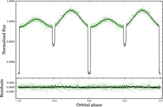
The Kepler Q0, Q1, Q2 and Q3 data of KOI-74, folded on the orbital period and binned into 2000 phase bins. The black curve shows a typical model fit to the data. The residuals of the data points after subtracting the model are shown in the bottom panel, binned into 2000 phase bins (green) and 200 phase bins (black).

Open in new tabDownload slide

Below, we discuss the various steps of our binary light-curve modelling.

3.1 Detrending of the Kepler data

We extracted the Kepler data from the pixel data, rather than using the pipeline output. We first normalized the data by dividing out an initial model fit, to be able to determine the trends in the data. Next, we detrended the data by dividing out exponentials fitted to the two obvious instrumental decays during Q2 and Q3. We removed 101 long-cadence points from the Q2 data, as well as 1299 short-cadence data points from the Q3 data, which were too severely affected by instrumental effects to allow for accurate detrending. We then divided out second-order polynomials fitted to each segment of the light curve. While fitting the polynomials, we flagged 184 points as >4σ outliers, in an iterative fashion, leaving 166 836 data points. We then folded the initial orbital fit back in. Finally, we binned the short-cadence data out of eclipse to long-cadence data since there are no binary signatures to be expected outside eclipse that require the time precision offered by short cadence. This way, the number of data points is reduced to 28 086.

Initial MCMC runs using this data set (see Section 3.4) showed, as expected, that there is no correlation between the adopted ephemerides (T₀ and P) and the other free parameters. We therefore decided to create a phase-folded version of the four months of short-cadence data to speed up the simulations. We rebinned the light curve into 1800-s bins out of eclipse and 30-s bins in eclipse, to be left with 1717 data points.

We assume that there is no background contamination in the Kepler data. We provide our final data sets in electronic form with this paper (see Supporting Information).

3.2 What can we learn from the Kepler light curve?

Fitting a light curve of a binary that shows a variety of effects (such as eclipses, ellipsoidal modulation and Doppler beaming) allows one to gain much information on the binary’s parameters. We first explore the potential before we discuss the actual light-curve fits in Section 3.4.

A first useful constraint comes from the measured fractional transit depth, which reveals the ratio of the radii of the two stars:

1

Given R₂/R₁ from the transit depth and T₁ from the spectral fit (Section 2), the eclipse depth provides information about T₂. Using blackbody approximations and neglecting the contribution of the companion out of eclipse, one finds

2

The eclipse duration t_e gives R₁/a as a function of the inclination i (assuming spherical stars):

3

(Russell 1912) with P being the orbital period and a the separation between the two binary components.

In case of corotation of the star with the binary orbit, the semi-amplitude of the ellipsoidal modulation can be approximated as3

4

(Morris & Naftilan 1993; Zucker et al. 2007) in which q=M₂/M₁ is the mass ratio of the two binary components, u₁ is the primary’s linear limb-darkening coefficient and τ₁ is its gravity-darkening coefficient.

With R₁/a determined from the eclipse duration (equation 3), q is then known as a function of i. In the case of KOI-74, the primary is not in corotation but is a rapid rotator, as already suggested by van Kerkwijk et al. (2010) and confirmed by all measurements of the rotational velocity (see Section 2). van Kerkwijk et al. (2010) argue that rapid rotation has a very significant impact on the ellipsoidal modulation amplitude. Kruszewski (1963) presented an expression for the Roche lobe potentials that accounts for the effects of asynchronous rotation. Although we will use this treatment in our light-curve models, we will be careful when interpreting the mass ratio derived from our light-curve modelling effort presented in Section 3.4. Our modelling set-up is such that the mass ratio is the only parameter that is only constrained by the ellipsoidal modulation amplitude. Therefore, if the expression for the ellipsoidal modulation is invalid (e.g. because it assumes instantaneous adjustment of the star’s surface to the ever-changing potential in the asynchronous case), this will manifest itself in the mass ratio being off.

The detection of Doppler beaming in the extremely accurate Kepler light curve (see van Kerkwijk et al. 2010) gives access to a second, independent, way to determine q as a function of i. For velocities much lower than the speed of light, the Doppler beaming amplitude is proportional to the radial velocity amplitude of the A-star:

5

(equation 2 in Bloemen et al. 2011). The beaming factor

6

(Loeb & Gaudi 2003) depends on the wavelength λ of the observation and on the spectrum of the star. We determine this factor for the case of KOI-74 in Section 3.3.

With M₁ given by the spectral type derived from spectroscopy (Section 2), and K₁ derived from the Doppler beaming amplitude (equation 5) or spectroscopy (Section 2), we get the following relation where q and i are the only unknowns:

7

This equation allows one to derive the mass ratio without relying on the amplitude of the ellipsoidal modulation (as long as the deformation of the primary is small enough not to affect the spectroscopic parameter determinations). The mass ratio q derived from the radial velocity amplitude using equation (7) is not influenced by the rapid rotation, contrary to the mass ratio that can be derived from the ellipsoidal modulation amplitude via equation (4).

Recently, Kaplan (2010) showed that one can use an effect similar to the Rømer delay to derive the radial velocity amplitude of the secondary, in double white dwarf binaries with circular orbits and mass ratios significantly different from 1. In such systems, a light-travel time difference causes the time between the primary and secondary eclipses to be different from P/2 by

8

in which c denotes the speed of light (see Kaplan 2010). After substitution of q=K₁/K₂, we find the following expression:

9

If we can measure this Rømer delay, it would allow us to derive the mass ratio in yet another way, this time independently from the mass of the primary which was estimated from spectral analysis. As far as we are aware, this technique has not yet been applied to any system in practice. KOI-74 is a good candidate to put the theory to the test, since the expected time difference is of the order of a minute.

3.3 Gravity-darkening, limb-darkening and Doppler beaming coefficients

The gravity-darkening coefficient (see e.g. Claret 2003) of the primary was calculated by integrating ATLAS model spectra (Castelli & Kurucz 2004) over the Kepler bandpass. We took into account the estimated reddening of E(B−V) = 0.15 (Kepler Input Catalog) by reddening the model spectra following Cardelli, Clayton & Mathis (1989). Reddening marginally influences the gravity-darkening coefficient because it is bandpass dependent. Assuming solar metallicity, v_turb= 2 km s⁻¹, T_eff= 9500 ± 250 K and log (g) = 4.3 ± 0.1, and using equation (1) from Bloemen et al. (2011), we found the gravity-darkening coefficient to be β_K= 0.55 ± 0.05. We have used a physical gravity-darkening coefficient of dlog T/dlog g= 0.25.

Using the same assumptions, we computed limb-darkening coefficients for the A-star. We adopted the four-parameter limb-darkening relation of Claret (2004, equation 5) with a₁= 0.576, a₂= 0.118, a₃=−0.039 and a₄=−0.016. For the white dwarf companion, we used a model atmosphere for a DA white dwarf with T_eff= 13 000 K and log g= 6.5 (Koester 2010) and found a₁= 0.372, a₂= 0.518, a₃=−0.540 and a₄= 0.178.

For the broad-band Kepler photometry, the wavelength-specific beaming factor (B in equation 5) has to be replaced by a bandpass-integrated photon-weighted beaming factor

10

(equation 3 in Bloemen et al. 2011), in which ε_λ is the response function of the Kepler bandpass and B is the monochromatic beaming factor (equation 6). Taking reddening into account, the beaming factor is found to be 〈B〉= 2.19 ± 0.04, which compares well with the van Kerkwijk et al. (2010) value of 2.21. For an unreddened spectrum, the beaming factor would be 〈B〉= 2.22 ± 0.04.

3.4 Modelling code and MCMC set-up

Our light-curve modelling code, lcurve (for a description of the code, see Copperwheat et al. 2010, appendix A), uses grids of points on the two binary components to calculate the total flux that is visible from the system at different orbital phases. It accounts for Doppler beaming, eclipses and transits, ellipsoidal modulation and reflection effects. The code can also account for lensing effects (implemented following Marsh 2001), which occur when the white dwarf transits the primary. In the models of KOI-74 presented here, however, we did not include these lensing effects. The white dwarf radius we would find by including lensing would be slightly larger but we estimate the difference at about 1 per cent only, which is far lower than the uncertainty on the parameter. In addition, estimation of the lensing requires knowledge of the mass of the white dwarf, which owing to the difficulty in deducing the mass ratio from the ellipsoidal variations, was not easily calculated during the MCMC runs.

A typical light-curve fit is shown in Fig. 3, together with the phase-folded light curve and the residuals. Because of the large difference in the radii of the stars, it turned out to be difficult to get the numerical noise at a lower level than the scatter on the observational data points of the superb Kepler light curve. The grid on the A-star would have to consist of millions of points to get to the required accuracy level, which is particularly difficult during the transits. We therefore replaced the grid of uniformly distributed points, at the transit phases, by a grid with a denser strip on the A-star at the region of the star that gets occulted during the white dwarf transits. A graphical representation of the grid is shown in Fig. 4. We used 92 716 points (on 270 latitude strips) on the A-star outside the transits and 178 468 points during the transits (adding 7 latitude and 4 longitude points per coarse grid point in the strip). The flux from the white dwarf was modelled with a 12 724-points grid (100 latitude strips) at all orbital phases.

Figure 4

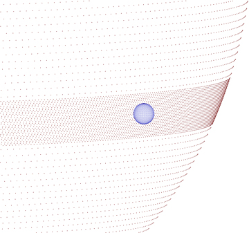
Illustration of the grids of points we used on the two binary components to model the light curve of KOI-74 (only about one point in four is shown on the A-star, and about one in 10 on the white dwarf). To achieve a high enough numerical precision, at the transit phases, a denser strip is used on the primary at the location where it gets occulted by the white dwarf. The system is shown with an inclination of 86°.4, at orbital phase 0.02.

Open in new tabDownload slide

To account for a possible detection of the Rømer delay, we introduced a δt parameter and computed the light curve at phase φ′ instead of the requested phase φ, with

11

This essentially results in a maximum Rømer delay of −δt at the phase of the eclipse, while the phase of the transit is untouched.

In an attempt to correctly model the ellipsoidal modulation taking into account the effects of rapid rotation, we implemented the adapted Roche lobe potentials as given by Kruszewski (1963). The modelling procedure, using MCMC simulations, is identical to the one used in Bloemen et al. (2011, sections 3.3 and 3.4) for the modelling of the light curve of KPD 1946+4340. In the initial runs using the full data set, the orbital period (P_orb), the time zero-point (T₀), the inclination (i), the temperature of the white dwarf (T₂), the mass ratio (q), the beaming factor (〈B〉) and the Rømer delay (δt) were kept as free parameters. The computation of one synthetic light curve at the 28 086 time points of the data set, for which we computed the light curve at about 127 000 phases to be able to account for the finite integration time of the observations, took about 5 min of CPU time. Due to the strong degeneracy between the inclination and the mass ratio, the MCMC chains took too much time to sample the whole parameter space. We therefore fixed the orbital period (P_orb) and the time zero-point (T₀) at the optimal values of the initial runs, and used the phase-folded light curve (see Section 3.1 for details) for the final runs.

To account for the finite integration times of the observations, we oversampled our light curves in time space. The 30-s phase bins during eclipses and transits were oversampled by a factor of 5, and the 1800-s phase bins out of eclipse by a factor of 3. For the oversampling, we approximated the effective integration time for each bin by ⁠, in which I is the integration time of the binned short-cadence data points (about 58 s) and x is the width of the bin (30 s or 1800 s). To explore the effects of rapid rotation, we ran MCMC chains assuming corotation (as in the case of KPD 1946+4340), as well as chains treating the spin rate as a free parameter with vsin i= 150 ± 10 km s⁻¹ as a prior. This prior was implemented as a constraint on (2πR/P) sin  i. In total, we computed over 450 000 light curves in the corotation chain, plus about 400 000 light curves in the fast rotation chain with a spectroscopic prior on the spin rate. Every tenth model that was computed was stored and used to determine the system parameters.

We set the limb-darkening coefficients to the values found in Section 3.3 and used priors on the flux-weighted temperature of the primary (T₁= 9500 ± 250 K, taken from spectroscopy, see Section 2), the gravity-darkening coefficient of the primary (β_K= 0.55 ± 0.05, see Section 3.3) and the radial velocity amplitude of the primary (K₁= 15.4 ± 0.3 km s⁻¹, taken from spectroscopy, see Section 2). If the amplitude of the Doppler beaming effect is consistent with the radial velocity amplitude, as was the case for KPD 1946+4340 (Bloemen et al. 2011), the results of the analysis will be identical when the prior on K₁ would be replaced by a prior on 〈B〉. In our approach, putting a prior on K₁ and treating 〈B〉 as a free parameter, we can judge whether the Doppler beaming effect has the expected amplitude by comparing the 〈B〉 that results from our MCMC analysis with the one found from atmosphere models in Section 3.3.

3.5 MCMC results and discussion

As can be seen in Fig. 3, the light-curve model fits the observed data very well. There is some structure in the residuals around the transit ingress and egress (around orbital phase 0.5), but it is barely significant. This structure can for example result from a small difference between the assumed limb-darkening coefficients (which were derived for a spherical star) and the true limb-darkening of the A-star. The parameters derived from our MCMC runs that account for the rapid rotation of the primary, using the prior on vsin i, are summarized in Table 2. Rowe et al. (2010) determined M₁= 2.2 ± 0.2 M_⊙ based on the spectral type. Using the evolutionary model grids of Briquet et al. (2011) and our spectroscopic determinations of T_eff and log g, we find the same result, which we adopted for our analysis. The results of the MCMC chains for the corotating case are nearly identical except for the derived mass ratios. The mass ratio from the models assuming corotation is also listed in the table, to allow for comparison with previously published values. The most important difference between our results and those previously published is that our inclination i= 87°.0 ± 0°.4 differs by ∼3σ from the value derived by Rowe et al. (2010), i= 88°.8 ± 0°.5. In that paper, the inclination was determined by fitting the eclipses and transits using the analytical formulae of Mandel & Agol (2002), which include limb darkening but not gravity darkening. Furthermore, it is possible that the authors did not account for the finite exposure times, which significantly smear out the eclipse ingresses and egresses in the long-cadence data they had available. Fitting only the 43 d of long-cadence data that Rowe et al. (2010) used, we find an uncertainty on the inclination of 0°.9, compared to their more optimistic value of 0°.5. The four months of short-cadence observations allowed us to determine the inclination more reliably.

Table 2

Open in new tab

Properties of KOI-74. The mass of the primary, the effective temperature and the rotational velocity are derived from spectroscopy. The other parameters are the result of our MCMC analysis of the Kepler data. The two different mass ratios are derived from the information contained in the ellipsoidal modulation amplitude (q_ell) and the radial velocity (q_RV). The mass of the secondary is derived using q_RV.

	Primary (A-star)	Secondary (white dwarf)
Porb (d)	5.188 675(4)
i (°)	87.0 ± 0.4
Teff (K)	9500 ± 250	14 500 ± 500
qell, corot	0.052 ± 0.004
qell, vsini	0.047 ± 0.004
qRV	0.104 ± 0.004
R	2.14 ± 0.08	0.044 ± 0.002
M	2.2 ± 0.2	0.228 ± 0.014
vsin i (km s−1)	150 ± 10	−
	−56 ± 17
〈B〉	2.24 ± 0.05	−

	Primary (A-star)	Secondary (white dwarf)
Porb (d)	5.188 675(4)
i (°)	87.0 ± 0.4
Teff (K)	9500 ± 250	14 500 ± 500
qell, corot	0.052 ± 0.004
qell, vsini	0.047 ± 0.004
qRV	0.104 ± 0.004
R	2.14 ± 0.08	0.044 ± 0.002
M	2.2 ± 0.2	0.228 ± 0.014
vsin i (km s−1)	150 ± 10	−
	−56 ± 17
〈B〉	2.24 ± 0.05	−

Table 2

Open in new tab

Properties of KOI-74. The mass of the primary, the effective temperature and the rotational velocity are derived from spectroscopy. The other parameters are the result of our MCMC analysis of the Kepler data. The two different mass ratios are derived from the information contained in the ellipsoidal modulation amplitude (q_ell) and the radial velocity (q_RV). The mass of the secondary is derived using q_RV.

	Primary (A-star)	Secondary (white dwarf)
Porb (d)	5.188 675(4)
i (°)	87.0 ± 0.4
Teff (K)	9500 ± 250	14 500 ± 500
qell, corot	0.052 ± 0.004
qell, vsini	0.047 ± 0.004
qRV	0.104 ± 0.004
R	2.14 ± 0.08	0.044 ± 0.002
M	2.2 ± 0.2	0.228 ± 0.014
vsin i (km s−1)	150 ± 10	−
	−56 ± 17
〈B〉	2.24 ± 0.05	−

	Primary (A-star)	Secondary (white dwarf)
Porb (d)	5.188 675(4)
i (°)	87.0 ± 0.4
Teff (K)	9500 ± 250	14 500 ± 500
qell, corot	0.052 ± 0.004
qell, vsini	0.047 ± 0.004
qRV	0.104 ± 0.004
R	2.14 ± 0.08	0.044 ± 0.002
M	2.2 ± 0.2	0.228 ± 0.014
vsin i (km s−1)	150 ± 10	−
	−56 ± 17
〈B〉	2.24 ± 0.05	−

The distribution of the inclination values in our MCMC runs using the prior on vsin i is shown in the bottom panel of Fig. 5. The two top panels of the figure show our radius estimates (relative to the separation of the two stars, a) as a function of the inclination. The blue points with error bars indicate the values found by van Kerkwijk et al. (2010), who did not derive the inclination independently but instead adopted the value of Rowe et al. (2010). Due to our lower preferred inclination, the radii inferred in our analysis are slightly larger than the ones obtained by van Kerkwijk et al. (2010).

Figure 5

Illustration of the correlation between the inclination of the system and the mass ratio and radii of the stars. The bottom panel shows the distribution of the models that were accepted in our MCMC runs that account for the rapid rotation of the primary. The dashed (dot–dashed) line indicates the 68 (95) per cent confidence interval. The black dots represent a random selection of the models. The blue dots with error bars show the results from van Kerkwijk et al. (2010). The red line on the mass ratio plot is the theoretical relation based on equations (3) and (4), assuming corotation. The blue line shows the mass ratio derived from K₁ (equation 7).

Open in new tabDownload slide

The third panel of Fig. 5 shows the mass ratio as a function of the inclination. The red line is the theoretical relation, assuming corotation, based on the constraints offered by the transit duration (equation 3) and the ellipsoidal modulation amplitude (equation 4). The distribution of points from our corotation runs falls nicely around this line (not shown). The blue line shows the mass ratio derived from the spectroscopic K₁, or equivalently, as we will see further in this section, the Doppler beaming amplitude. The discrepancy between the mass ratios derived from the ellipsoidal modulation amplitude on the one hand, and from the radial velocity information on the other hand, was already noted by van Kerkwijk et al. (2010). The results of the models that account for rapid rotation of the primary are plotted with black dots. It is striking that these models result in lower rather than higher mass ratios, thus only increasing the discrepancy compared to the models assuming corotation. The lower preferred inclination value also contributes to the increase in the discrepancy between the two mass ratios, compared to the discrepancy shown by van Kerkwijk et al. (2010). This can easily be understood: as i gets lower, R₁/a has to increase to make the model fit the observed transit duration (equation 3); but a higher R₁/a would lead to a higher ellipsoidal modulation amplitude, which is then compensated in the simulations by lowering q_ell (equation 4).

The beaming factor derived from the MCMC chains, 〈B〉= 2.24 ± 0.05, agrees with the beaming factor derived from spectroscopy in Section 3.3 (〈B〉= 2.19 ± 0.04, taking reddening into account). We could thus have modelled the binary equally well without spectroscopic radial velocity information, just relying on the Doppler beaming amplitude in the Kepler light curve, verifying van Kerkwijk et al. (2010)’s approach.

One can argue that the mass ratios determined from the ellipsoidal modulation amplitude and radial velocity information can be brought into agreement by assuming a high contamination of the Kepler light curve by background stars, since this would increase the observed ellipsoidal modulation amplitude. The consistency between the observed Doppler beaming amplitude (which would also increase if one assumes a higher contamination) and the spectroscopic radial velocity amplitude, however, implies that our assumption of no background contamination in the Kepler light curve has to be correct up to a few per cent.

We were also able to measure the Rømer delay at δt=−56 ± 17 s, as can be seen on the distribution plot from our MCMC chains in Fig. 6. The expected Rømer delay for a mass ratio of q= 0.104 is δt=−63.2 ± 1.2 s, while for q= 0.050 we would expect δt=−139 ± 3 s (the error bars account for the uncertainty on K₁ measured from spectroscopy). The Rømer delay estimates only depend on P_orb, K₁ and the mass ratio. With P_orb and K₁ firmly established from both spectroscopy and photometry, the measurement of the delay proves that the true mass ratio of the system is the one derived from the radial velocity amplitude, under the condition that the orbit is circular. Note that while K₁ can be derived from the Doppler beaming amplitude, a measurement of the Rømer delay allows one to also derive K₂ directly from the light curve if M₁ is known.

Figure 6

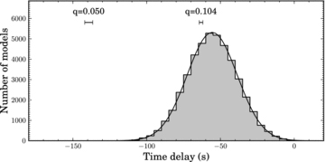
Distribution of the Rømer delay as fitted by our MCMC runs. The delays expected for mass ratios of q= 0.050 and 0.104 are indicated for comparison.

Open in new tabDownload slide

3.6 Variability in residuals

We performed a time–frequency analysis on the residuals of the short-cadence data after subtracting our best model. The time–frequency diagram is shown in Fig. 7. We detected significant variability (following the criteria given in Degroote et al. 2009), but all at low amplitudes (∼10 parts per million). We found variability with periods of ∼3 d, which is a known instrumental artefact (see Christiansen et al. 2011). We also found variability with a period of 0.5918 ± 0.0015 d, with an amplitude that changes in time (see Fig. 7). van Kerkwijk et al. (2010) suggested that this signal could be associated with the spin period of the A-star. Given our spectroscopic value for vsin i and the radius determination from our light-curve analysis, we expect the spin period of the A-star to be 0.72 ± 0.06 d, which differs by 2σ from the detected periodicity.

Figure 7

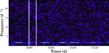
Time–frequency analysis of the residuals of the short-cadence data after subtracting our best-fitting binary light-curve model. The observed variability at ∼1.3 d⁻¹ might be related to the spin period of the primary star.

Open in new tabDownload slide

We detected additional variability of similar amplitude in the long-cadence Q2 data at frequencies between 15 and 20 d⁻¹. We could find a similar signal in the observations of KIC 6889190, which is observed on the same CCD close to KOI-74, and it can be removed successfully using the cotrending basis vectors technique described in Christiansen et al. (2011) (Tom Barclay, private communication). This confirms that it is instrumental in nature.

We did not find significant residual power at the orbital period which proves that the lcurve model fits the data very well.

4 SUMMARY

We have analysed 212 d of Kepler data (Q0, Q1, Q2 and Q3) of the eclipsing binary KOI-74, as well as supporting spectroscopic observations. We modelled the light curve using the lcurve code, accounting for ellipsoidal modulation, reflection effects, Doppler beaming, Rømer delay, eclipses and transits. Using MCMC simulations, we determined various system parameters of KOI-74, which are summarized in Table 2. We find a lower orbital inclination of i= 87°.0 ± 0°.4 compared to the discovery paper and first analysis presented by Rowe et al. (2010) and adopted by van Kerkwijk et al. (2010), i= 88°.8 ± 0°.5. The difference propagates to our values of other parameters such as the radii. It lowers the mass ratio derived from the ellipsoidal modulation amplitude to q= 0.052 ± 0.004 assuming corotation or q= 0.047 ± 0.004 accounting for a rapidly rotating primary (using vsin i= 150 ± 10 km s⁻¹ as a prior).

The amplitude of the observed Doppler beaming, which makes the primary become brighter when the star moves in the direction of the Kepler satellite in its orbit, is in perfect agreement with what is expected from the spectral type and radial velocity amplitude of the star, which we determined to be K₁= 15.4 ± 0.3 km s⁻¹ from spectroscopy. From the primary’s mass of the mass ratio derived from the radial velocity is q= 0.104 ± 0.004.

We also report the first detection of Rømer delay in a light curve of a compact binary. This delay, which amounts to 56 ± 17 s, is exactly as long as one would expect for a mass ratio of q∼ 0.1, and is in contradiction with the lower mass ratio derived from the ellipsoidal modulation amplitude. van Kerkwijk et al. (2010) preferred the mass ratio derived from the Doppler beaming amplitude over the mass ratio derived from the ellipsoidal modulation amplitude. We find that the spectroscopic radial velocity amplitude as well as the Rømer delay leaves no doubt that this was indeed the correct assumption, and that the secondary of KOI-74 is a low-mass white dwarf.

As a result of our lower preferred orbital inclination value, the discrepancy between the mass ratio determined from the ellipsoidal modulation amplitude and the higher mass ratio determined from radial velocity information or Rømer delay has increased compared to van Kerkwijk et al. (2010), and now amounts to a factor of 2. Our attempt to account for the effect of the rapid rotation of the primary increased the discrepancy even further. Our results imply that one has to be very cautious when adopting mass ratio estimates derived from the ellipsoidal modulation amplitude, in particular if there is no firm proof of corotation. We are not aware of any theoretical explanation of the reduction in ellipsoidal modulation as a result of rapid asynchronous rotation.

The authors thank the reviewer, Marten van Kerkwijk, for his detailed and helpful comments on the paper. SB, PD and CA acknowledge the KITP staff of UCSB for their warm hospitality during the research programme ‘Asteroseismology in the Space Age’. SB acknowledges the travel grant (V446211N) he received from the Fund for Scientific Research of Flanders (FWO), Belgium, for his stay at KITP. This research was supported in part by the National Science Foundation, USA, under grant no. NSF PHY05-51164. The HERMES project and team acknowledge support from the Fund for Scientific Research of Flanders (FWO), Belgium, the Research Council of K.U. Leuven, Belgium, the Fonds National Recherches Scientifique (FNRS), Belgium, the Royal Observatory of Belgium, the Observatoire de Genève, Switzerland, and the Thüringer Landessternwarte Tautenburg, Germany. The research leading to these results has received funding from the European Research Council under the European Community’s Seventh Framework Programme (FP7/2007–2013)/ERC grant agreement no. 227224 (PROSPERITY), as well as from the Research Council of K.U. Leuven grant agreement GOA/2008/04. During this research TRM, EB, CMC, SP and BTG were supported under a grant from the UK’s Science and Technology Facilities Council (STFC, ST/1001719/1). The authors acknowledge the Kepler team. Funding for this Discovery mission is provided by NASA’s Science Mission Directorate. For the simulations we used the infrastructure of the VSC – Flemish Supercomputer Center, funded by the Hercules Foundation and the Flemish Government – department EWI. This research has made use of SIMBAD, maintained by the Centre de Données astronomiques de Strasbourg; the arXiv preprint service, maintained and operated by the Cornell University Library; and NASA’s Astrophysics Data System (ADS).

Footnotes

REFERENCES

SUPPORTING INFORMATION

Additional Supporting Information may be found in the online version of this article.

HERMES_balmer.dat. Radial velocities measured from Balmer lines in HERMES spectra.

ISIS_balmer.dat. Radial velocities measured from Balmer lines in ISIS spectra.

HERMES_mgii.dat. Radial velocities measured from theMgII line in HERMES spectra.

ISIS_mgii.dat. Radial velocities measured from the MgII line in ISIS spectra.

Detrended_lc.dat. Detrended light curve used for the MCMC analysis.

Folded_lc.dat. Phase-folded light curve used for the MCMC analysis.

Please note:Wiley-Blackwell are not responsible for the content or functionality of any supporting materials supplied by the authors. Any queries (other than missing material) should be directed to the corresponding author for the article.

Author notes