


Abstract
An analytical model predicting the growth rates, the absolute growth times and the saturation values of the magnetic field strength within galactic haloes is presented. The analytical results are compared to cosmological magnetohydrodynamics (MHD) simulations of Milky Way-like galactic halo formation performed with the N-body/spmhd code gadget. The halo has a mass of ≈3 × 10¹² M⊙ and a virial radius of ≈270 kpc. The simulations in a Λ cold dark matter (ΛCDM) cosmology also include radiative cooling, star formation, supernova feedback and the description of non-ideal MHD.
A primordial magnetic seed field ranging from 10−10 to 10−34 G in strength agglomerates together with the gas within filaments and protohaloes. There, it is amplified within a couple of hundred million years up to equipartition with the corresponding turbulent energy. The magnetic field strength increases by turbulent small-scale dynamo action. The turbulence is generated by the gravitational collapse and by supernova feedback. Subsequently, a series of halo mergers leads to shock waves and amplification processes magnetizing the surrounding gas within a few billion years. At first, the magnetic energy grows on small scales and then self-organizes to larger scales. Magnetic field strengths of ≈10−6 G are reached in the centre of the halo and drop to ≈10−9 G in the intergalactic medium.
Analysing the saturation levels and growth rates, the model is able to describe the process of magnetic amplification notably well and confirms the results of the simulations.
1 INTRODUCTION
The Λ cold dark matter (ΛCDM) model is the standard tool describing the evolution of the universe (Komatsu et al. 2011). Quantum fluctuations in the primordial energy distribution develop into the condensing matter and trigger gravitational instabilities. Dark matter clumps in filaments and protohaloes, and subsequently baryonic matter falls into the potential wells of the dark matter, thereby forming the first stars and galaxies. In a hierarchical process of merger events, larger structures grow (White & Rees 1978; White & Frenk 1991). Numerical simulations of structure formation within a ΛCDM universe show good agreement between the calculated and the observed distribution of matter and structures (Springel et al. 2005; Springel, Frenk & White 2006). However, cosmic magnetic fields are still widely neglected in these kinds of simulations, although their presence can influence the dynamics of an astrophysical system significantly.
Observations reveal strong magnetic fields of μG strength in late-type galaxies (for reviews on cosmic magnetism, see e.g. Beck et al. 1996; Widrow 2002; Kulsrud & Zweibel 2008, and references therein). The energy density of these magnetic fields is comparable to other dynamically important energy densities, i.e. the magnetic field seems to be in equipartition with them. Neronov & Vovk (2010) also find strong magnetic fields permeating the intergalactic medium (IGM). The IGM magnetic fields are highly turbulent (Ryu et al. 2008) and their strength is estimated to be of the order of nG (Kronberg et al. 2008). Additionally, magnetic fields of μG strength can be found in high-redshift galaxies (Bernet et al. 2008). Also, there is evidence of highly magnetized damped Lyman α systems at redshift ≈2, which act as building blocks for galactic systems (Wolfe, Gawiser & Prochaska 2005).
The origin of these magnetic fields is still unclear. Global primordial magnetic fields can be seeded by battery processes in the early universe (Biermann 1950; Mishustin & Ruzmaikin 1972; Zel’dovich, Ruzmaikin & Sokoloff 1983; Huba & Fedder 1993). Alternatively, seed fields can be generated by phase transitions after the big bang or various other mechanisms (see Widrow 2002 for a review).
In a subsequent process, these weak seed fields of sometimes ≤10−20 G have to be amplified to the observed values. Lesch & Chiba (1995) demonstrate the possibility of strong magnetic fields at high redshifts through battery processes and protogalactic shear flow amplification. The presence of strong μG galactic magnetic fields is commonly explained by galactic dynamos converting angular momentum into magnetic energy in differentially rotating discs. The two main theories are the α–ω dynamo (Ruzmaikin et al. 1979) or the cosmic ray-driven dynamo (Lesch & Hanasz 2003; Hanasz et al. 2009). For reviews of dynamo theory, see Brandenburg & Subramanian (2005) or Shukurov (2007). However, these dynamos operate on time-scales (e-folding time, not absolute amplification time) of the order of 108 yr and require a differentially rotating galactic disc. Hence, irregular galaxies at high redshift have to be magnetized by another process. Another possible magnetization process is the ‘cosmic dynamo’ as given by Dubois & Teyssier (2010). Within their approach, the universe is magnetized by gravitational instabilities, galactic dynamos and wind-driven outflows of gas at times of violent star formation activity.
Small-scale dynamos operate on time-scales of the order of 106 yr through random and turbulent shear flow motions (Biermann & Schlüter 1951). Magnetic energy increases exponentially on small scales first by stretching, twisting and folding the magnetic field lines by random motions and then organizing them on the largest turbulent eddy scale (Zel’dovich et al. 1983; Kulsrud & Anderson 1992; Kulsrud et al. 1997; Malyshkin & Kulsrud 2002; Schekochihin et al. 2002, 2004; Schleicher et al. 2010). Galaxy mergers are a natural part of the bottom-up picture of the growth of structures in the universe. Kotarba et al. (2010, 2011) and Geng et al. (2012) show that turbulence induced during galactic major and minor mergers is able to amplify magnetic fields in galaxies and in the IGM up to equipartition between the magnetic and turbulent energy density, as expected from the small-scale dynamo theory. This theory is a good method to describe the amplification processes and corresponding time-scales (e.g. Arshakian et al. 2009). However, galactic dynamos are still inevitable to explain the regularity of galactic magnetic fields and their spiral structure, which are revealed by observations.
Analytical calculations and cosmological simulations of structure formation including the evolution of magnetic fields can give new insights in the physical processes of creating, amplifying and saturating magnetic fields in the universe on all kinds of scales.
In this work, an analytical model predicting the growth rates, the absolute growth times and the saturation values of the magnetic field strength within galactic haloes is presented. The analytical results are compared to cosmological MHD simulations of Milky Way-like galactic halo formation including star formation and non-ideal MHD. It is shown that the analytical model and the cosmological simulations agree notably well for different initial, primordial magnetic seed fields spanning a range of 25 orders of magnitudes.
This paper is organized as follows. The analytical calculations are shown in Section 2. Section 3 briefly describes the numerical method. In Section 4, the cosmological initial conditions and the magnetic seed field are presented. A detailed analysis of the performed simulations and the magnetic field amplification is given in Section 5. Section 6 compares the numerical results with the analytical description. The main results are summarized in Section 7.
2 ANALYTICAL DESCRIPTION
This section gives an analytical approach describing the behaviour of the magnetic field strength during halo formation. In order to derive an analytical model, expressions for the cosmological decay, the exponential amplification process, the saturation and the relaxing decay of the magnetic field strength are needed. For large hydrodynamical Reynolds numbers, a stationary flow transits from the laminar regime into the turbulent regime and becomes unstable. Hence, an overview of the characteristics of a non-stationary perturbated magnetic field in such an unstable flow in a cosmological context is given.
2.1 Local perturbation ansatz
 (e.g. the effective adiabatic index is γadi= 4/3 for isotropic compression) can still occur. This would result in the magnetic energy density first to shoot over the turbulent energy density (γadi= 1), and then decay towards the saturation level. However, this effect is too small to be significant. Now, to account for the saturation of the magnetic field at the equipartition level, Γ is amended (Belyanin et al. 1993) as follows:
 , equation (9) has the solution (Landau & Lifshitz 1959):
 is the mean-square turbulent velocity. From equation (7), Kulsrud et al. (1997) find for the growth rate γ:
These small-scale dynamos operate whenever turbulent and random motions and shear flows are stretching, twisting and folding the magnetic field lines (Zel’dovich et al. 1983; Schleicher et al. 2010). Field lines come close on small scales first, and hence the magnetic energy increases at first on small scales. The amplification is dominated by the turbulent dynamo action and effects resulting from compression can be neglected within this model.
2.2 Cosmological evolution and decay
 can be derived (Longair 2008):
Parameters used for the ΛCDM cosmology.
| Matter density | ΩM | 0.3 |
| Dark energy density | ΩΛ | 0.7 |
| Total density | Ω0 | 1.0 |
| Hubble constant | H0 | 70 km s−1 Mpc−1 |
| Matter density | ΩM | 0.3 |
| Dark energy density | ΩΛ | 0.7 |
| Total density | Ω0 | 1.0 |
| Hubble constant | H0 | 70 km s−1 Mpc−1 |
In the beginning, the term a(t)−2 dominates and results in the cosmological dip at high redshifts. Then, the magnetic energy increases with e 2γt(a) during the gravitational collapse and due to star formation-induced turbulence. This growth stops when equipartition is reached, since non-linear effects are truncating γ. Finally, when the system is relaxing and the turbulence is decaying, the magnetic field will also decay as a(t)−2 corresponding to a power-law decay with Bt∼t−4/3. This decay is slightly stronger compared to the Bt∼t−5/4 decay given by Landau & Lifshitz (1959) or George (1992) for the final stages of decaying kinematic turbulence (assuming that the magnetic energy decays with the same power law as the turbulent energy, which is an approximation). The final stage of decay is reached by the time, when the Reynolds number becomes sufficiently small. This happens when the back-reaction of the magnetic field on the velocity field suppresses turbulent motions and also magnetic amplification and the system relaxes. Subramanian, Shukurov & Haugen (2006) found the power-law decay to set in already for Reynolds numbers still as large as Re≈ 100 in galaxy clusters.
2.3 Numerical parameters
Equation (18) contains four free parameters: vturb, lturb, ηturb and ρ. The numerical values for these parameters have to be taken from observations or extracted from numerical simulations. Table 2 shows the values used in this work. These values correspond to a time-scale (e-folding time) of τ= 1/γ≈ 90 Myr and a saturation value of  at redshift 0. Note that these numerical parameters are constant mean estimates and do not reflect the time and spatial details of the simulations, but nevertheless are a good approximation.
Parameters used for the calculation of the analytical growth function (physical units).
| Turbulent length | lturb | 25 kpc |
| Turbulent velocity | vturb | 75 km s−1 |
| Turbulent dissipation | ηturb | 1030 cm2 s−1 |
| Gas density | ngas | 10−5 cm−3 |
| Turbulent length | lturb | 25 kpc |
| Turbulent velocity | vturb | 75 km s−1 |
| Turbulent dissipation | ηturb | 1030 cm2 s−1 |
| Gas density | ngas | 10−5 cm−3 |
Estimating values for vturb and lturb is quite challenging, as the densities, velocities and length scales in galactic haloes range over many orders of magnitude. Therefore, such values can only be associated with typical values within galactic haloes (see Section 6 for a discussion which values reflect best the simulations).
Fig. 1 shows growth curves as a function of redshift for a wide range of values of these parameters. In each panel, three parameters are held constant (see Table 2), while the fourth parameter is varied. As indicated by the presented calculations, vturb, lturb and ηturb affect the growth rate γ, while vturb and ρ affect the saturation value Bsat. Depending on the parameter configuration, the time-scale ranges from of the order of 106 to 108 yr and the saturation value for the magnetic field strength varies from 10−5 to 10−8 G.
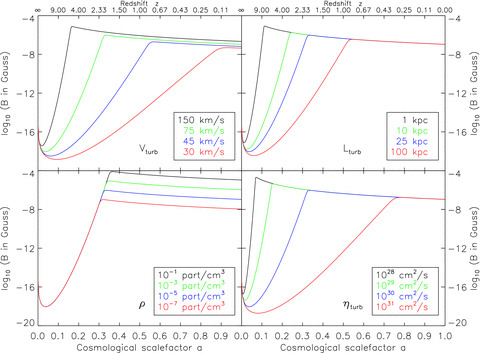
Analytical growth curves for the magnetic field amplitude as a function of redshift for different numerical parameters. In each panel, one parameter is varied, while the other parameters are held constant. Differences in the growth rates and saturation levels can be seen.
3 NUMERICAL METHODS
The simulations in this work are performed with the N-body/spmhd code gadget (Springel, Yoshida & White 2001b; Springel 2005; Dolag & Stasyszyn 2009). gadget uses a formulation of sph, in which both energy and entropy are conserved (Springel & Hernquist 2002). For recent reviews on the sph and spmhd methods, see Springel (2010) and Price (2012). Additionally, subfind (Springel et al. 2001a; Dolag et al. 2009) is applied to identify haloes and subhaloes and to calculate their respective centre locations and virial radii.

The magnetic field back-reacts on the velocity field via the Lorentz force. To account for the tensile instability (see Dolag & Stasyszyn 2009; Price 2012, for details) in spmhd, the unphysical numerical divergence force is subtracted from the equation of motion following an approach by Børve, Omang & Trulsen (2001). Similar to Kotarba et al. (2010), a limiter is applied to ensure that the correction force does not exceed the Lorentz force to avoid instabilities.
To ensure a proper evolution of the magnetic field in numerical simulations, it is of fundamental interest to maintain the ∇·B= 0 constraint. In particular, an erroneous calculation can lead to unphysical sources and sinks of magnetic energy. The mhd gadget code keeps these numerical errors to a minimum. For a detailed discussion, see Dolag & Stasyszyn (2009) and Section 5.3.
The implementation of MHD in gadget was successfully employed for the study of the magnetic field evolution during star formation (Bürzle et al. 2011a,b), in isolated (Kotarba et al. 2009) and interacting galaxies (Kotarba et al. 2010, 2011; Geng et al. 2012) and in galaxy clusters (Donnert et al. 2009).
Also, the Springel & Hernquist (2003a) star formation model is applied. It describes radiative cooling, ultraviolet (UV) background heating and supernova feedback in a consistent two-phase sub-resolution model for the interstellar medium. Cold clouds with a fixed temperature of TCC are embedded into a hot ambient medium at pressure equilibrium. These cold clouds are evaporating with an efficiency parameter of A and form stars on a time-scale of tSF, once they reach a density threshold of ρth. A fraction β of these stars is expected to die instantly as supernovae, heating the gas with a temperature of TSN. Additionally, the hot phase is losing energy via cooling, which is modelled assuming a primordial gas composition (hydrogen 76 per cent and helium 24 per cent) with a temperature floor of 50 K (for details see Katz,Weinberg & Hernquist 1996). The cooling only depends on density and temperature, but not on metallicity. This star formation model leads to a self-regulated cycle of cooling, star formation and feedback in the gas.
Table 3 shows the numerical values of these parameters used in the simulations, which are performed without galactic winds. These numbers are chosen to reproduce the Kennicutt–Schmidt law between surface density and surface star formation rate (Schmidt 1959; Kennicutt 1998).
Parameters for the star formation model (Springel & Hernquist 2003a) used in the simulations.
| Multi-phase model parameters | ||
| Gas consumption time-scale | tSF | 2.1 Gyr |
| Number density threshold | nth | 0.13 cm−3 |
| Mass fraction of massive stars | β | 10 per cent |
| Evaporation parameter | A | 1000 |
| Effective supernova temperature | TSN | 108 K |
| Temperature of cold clouds | TCC | 1000 K |
However, for simulations of the turbulent small-scale dynamo, the precise details of the star formation scheme are largely unimportant. Cooling is required to obtain higher gas densities and smaller spatial scales in order to start efficient dynamo action. Furthermore, feedback-driven turbulence will contribute to the gravitationally driven turbulence and raise the growth rates of the magnetic field strength.
4 SET-UP
4.1 Dark matter initial conditions
The presented simulations start from cosmological initial conditions introduced by Stoehr et al. (2002). The starting point is a large ΛCDM dark matter-only simulation box run with the gadget code at different resolutions. The index of the power spectrum of the initial fluctuations is n= 1 and the fluctuation amplitude is σ8= 0.9 (see Stoehr et al. 2002 for details). In a ‘typical’ region of the universe, a Milky Way-like dark matter halo is identified. The resulting simulations (with increasing resolution) are labelled GA0, GA1 and GA2, and contain 13 603, 123 775 and 1055 083 dark matter particles, respectively, inside R200, which is the radius enclosing a mean density 200 times the critical density (virial radius).
The forming dark matter halo is comparable to the halo of the Milky Way in mass (≈3 × 10¹² M⊙) and size (≈270 kpc). The halo was selected to have no major merger after a redshift of ≈1, and a subhalo population comparable to the satellite population of the Milky Way was also found. More details about the properties of this halo can be found in Stoehr et al. (2002, 2003) and Stoehr (2006). Hence, GA0, GA1 and GA2 provide ideal initial conditions to investigate the evolution of magnetic fields in a galactic halo, similar to the Milky Way.
4.2 Gas and magnetic field
To add a baryonic component, the high-resolution dark matter particles are split into an equal amount of gas and dark matter particles. The mass of the initial dark matter particle is split according to the cosmic baryon fraction, conserving the centre of mass and the momentum of the parent dark matter particle. The new particles are displaced by half the mean inter-particle distance.
 and an electron current density
  . Then, electrons and protons are moving at different speeds in the plasma, reacting differently to perturbations. This results in currents and a non-ideal term in the induction equation of the form:
Actually, the magnetic energy should be distributed to the different scales of the simulation, resulting in a magnetic spectrum. However, this spectral property of the magnetic field can be neglected for magnetic energy densities  sufficiently smaller than the kinetic energy density ɛkin=ρv2/2 (weak-field approximation). In this limit, the magnetic field B will be frozen into the velocity field v and follow its evolution. Hence, only the amplitude of the magnetic seed field is relevant, but not its direction.
Table 4 shows the simulations performed, which can be grouped into three sets. First, low-resolution simulations GA0 are used for a numerical study of different seed field strengths ranging from 10−10 to 10−34 G and being uniform in the x-direction. Additionally, a run of GA0 with a seed field in the y-direction is shown to confirm the neglectability of the magnetic seed field direction. Secondly, for the seed field with the strength of 10−18 G, higher resolution runs GA1 and GA2 are added to analyse the influence of the numerical resolution on the evolution of the magnetic field. Furthermore, a special run of GA1 is performed to study the influence of the modelled star formation on the evolution of the magnetic field. Finally, to study the influence of magnetic fields on the existing simulations, additional runs with only hydrodynamics are obtained.
Set-up of the different simulations. The table lists whether star formation and cooling (SF/cool.) is applied, the number of gas (NGas) and dark matter particles (NDM), the mass of the gas (MGas) and dark matter particles (MDM), as well as the initial magnetic field orientation and strength for all simulated scenarios, respectively.
| Scenario | SF/cool. | NGas | NDM |  |  |  |  (G) (G) |
| ga0_bx0 | Yes | 68 323 | 68 323 | 2.6 × 10⁷ | 1.4 × 10⁸ | – | 0 |
| ga0_bx10 | Yes | 68 323 | 68 323 | 2.6 × 10⁷ | 1.4 × 10⁸ | x | 10−10 |
| ga0_bx14 | Yes | 68 323 | 68 323 | 2.6 × 10⁷ | 1.4 × 10⁸ | x | 10−14 |
| ga0_bx18 | Yes | 68 323 | 68 323 | 2.6 × 10⁷ | 1.4 × 10⁸ | x | 10−18 |
| ga0_by18 | Yes | 68 323 | 68 323 | 2.6 × 10⁷ | 1.4 × 10⁸ | y | 10−18 |
| ga0_bx22 | Yes | 68 323 | 68 323 | 2.6 × 10⁷ | 1.4 × 10⁸ | x | 10−22 |
| ga0_bx26 | Yes | 68 323 | 68 323 | 2.6 × 10⁷ | 1.4 × 10⁸ | x | 10−26 |
| ga0_bx30 | Yes | 68 323 | 68 323 | 2.6 × 10⁷ | 1.4 × 10⁸ | x | 10−30 |
| ga0_bx34 | Yes | 68 323 | 68 323 | 2.6 × 10⁷ | 1.4 × 10⁸ | x | 10−34 |
| ga1_bx0 | Yes | 637 966 | 637 966 | 2.8 × 10⁶ | 1.5 × 10⁷ | – | 0 |
| ga1_bx18 | Yes | 637 966 | 637 966 | 2.8 × 10⁶ | 1.5 × 10⁷ | x | 10−18 |
| ga1_bx18_nosf | No | 637 966 | 637 966 | 2.8 × 10⁶ | 1.5 × 10⁷ | x | 10−18 |
| ga2_bx0 | Yes | 5953 033 | 5953 033 | 3.0 × 10⁵ | 1.6 × 10⁶ | – | 0 |
| ga2_bx18 | Yes | 5953 033 | 5953 033 | 3.0 × 10⁵ | 1.6 × 10⁶ | x | 10−18 |
| Scenario | SF/cool. | NGas | NDM | | | | (G) |
| ga0_bx0 | Yes | 68 323 | 68 323 | 2.6 × 10⁷ | 1.4 × 10⁸ | – | 0 |
| ga0_bx10 | Yes | 68 323 | 68 323 | 2.6 × 10⁷ | 1.4 × 10⁸ | x | 10−10 |
| ga0_bx14 | Yes | 68 323 | 68 323 | 2.6 × 10⁷ | 1.4 × 10⁸ | x | 10−14 |
| ga0_bx18 | Yes | 68 323 | 68 323 | 2.6 × 10⁷ | 1.4 × 10⁸ | x | 10−18 |
| ga0_by18 | Yes | 68 323 | 68 323 | 2.6 × 10⁷ | 1.4 × 10⁸ | y | 10−18 |
| ga0_bx22 | Yes | 68 323 | 68 323 | 2.6 × 10⁷ | 1.4 × 10⁸ | x | 10−22 |
| ga0_bx26 | Yes | 68 323 | 68 323 | 2.6 × 10⁷ | 1.4 × 10⁸ | x | 10−26 |
| ga0_bx30 | Yes | 68 323 | 68 323 | 2.6 × 10⁷ | 1.4 × 10⁸ | x | 10−30 |
| ga0_bx34 | Yes | 68 323 | 68 323 | 2.6 × 10⁷ | 1.4 × 10⁸ | x | 10−34 |
| ga1_bx0 | Yes | 637 966 | 637 966 | 2.8 × 10⁶ | 1.5 × 10⁷ | – | 0 |
| ga1_bx18 | Yes | 637 966 | 637 966 | 2.8 × 10⁶ | 1.5 × 10⁷ | x | 10−18 |
| ga1_bx18_nosf | No | 637 966 | 637 966 | 2.8 × 10⁶ | 1.5 × 10⁷ | x | 10−18 |
| ga2_bx0 | Yes | 5953 033 | 5953 033 | 3.0 × 10⁵ | 1.6 × 10⁶ | – | 0 |
| ga2_bx18 | Yes | 5953 033 | 5953 033 | 3.0 × 10⁵ | 1.6 × 10⁶ | x | 10−18 |
Set-up of the different simulations. The table lists whether star formation and cooling (SF/cool.) is applied, the number of gas (NGas) and dark matter particles (NDM), the mass of the gas (MGas) and dark matter particles (MDM), as well as the initial magnetic field orientation and strength for all simulated scenarios, respectively.
| Scenario | SF/cool. | NGas | NDM | | | | (G) |
| ga0_bx0 | Yes | 68 323 | 68 323 | 2.6 × 10⁷ | 1.4 × 10⁸ | – | 0 |
| ga0_bx10 | Yes | 68 323 | 68 323 | 2.6 × 10⁷ | 1.4 × 10⁸ | x | 10−10 |
| ga0_bx14 | Yes | 68 323 | 68 323 | 2.6 × 10⁷ | 1.4 × 10⁸ | x | 10−14 |
| ga0_bx18 | Yes | 68 323 | 68 323 | 2.6 × 10⁷ | 1.4 × 10⁸ | x | 10−18 |
| ga0_by18 | Yes | 68 323 | 68 323 | 2.6 × 10⁷ | 1.4 × 10⁸ | y | 10−18 |
| ga0_bx22 | Yes | 68 323 | 68 323 | 2.6 × 10⁷ | 1.4 × 10⁸ | x | 10−22 |
| ga0_bx26 | Yes | 68 323 | 68 323 | 2.6 × 10⁷ | 1.4 × 10⁸ | x | 10−26 |
| ga0_bx30 | Yes | 68 323 | 68 323 | 2.6 × 10⁷ | 1.4 × 10⁸ | x | 10−30 |
| ga0_bx34 | Yes | 68 323 | 68 323 | 2.6 × 10⁷ | 1.4 × 10⁸ | x | 10−34 |
| ga1_bx0 | Yes | 637 966 | 637 966 | 2.8 × 10⁶ | 1.5 × 10⁷ | – | 0 |
| ga1_bx18 | Yes | 637 966 | 637 966 | 2.8 × 10⁶ | 1.5 × 10⁷ | x | 10−18 |
| ga1_bx18_nosf | No | 637 966 | 637 966 | 2.8 × 10⁶ | 1.5 × 10⁷ | x | 10−18 |
| ga2_bx0 | Yes | 5953 033 | 5953 033 | 3.0 × 10⁵ | 1.6 × 10⁶ | – | 0 |
| ga2_bx18 | Yes | 5953 033 | 5953 033 | 3.0 × 10⁵ | 1.6 × 10⁶ | x | 10−18 |
5 SIMULATIONS
This section presents the results obtained from the numerical simulations introduced above. Contour images of different quantities are created by projecting the spmhd data in a comoving  cube on a 5122 grid using the code P-smac2 (Donnert et al., in preparation).
5.1 Morphological and magnetic evolution
An overview of the different stages of structure formation and their implications on the magnetic field is shown in Fig. 2. First, dark matter protohaloes and filaments are formed at redshift z≈ 30–10, and baryonic matter falls into the potential wells. Within these structures, the frozen-in magnetic field gets compressed. For isotropic compression, this leads to B∼ρ2/3. Note that perpendicular compression of the magnetic field lines would lead to B∼ρ. Due to the cosmological expansion, the magnetic field strength outside these protohaloes decreases with a−2. Turbulence is mainly created by the gravitational collapse. Secondly, as the gas density increases in the first structures, the threshold density is reached and star formation sets in at redshift ≈10, further enhancing the existing turbulence and consuming the available gas. In these dense regions, small-scale dynamo action starts, increasing the magnetic field strength exponentially, i.e. B∼ eγt with the growth rate γ (see also Section 2). Merger events will create shockwaves propagating into the IGM, possibly amplifying the magnetic field by compression and small-scale dynamo action. As equipartition is reached, the system relaxes and turbulent motions will decay, with additionally the magnetic field decaying.
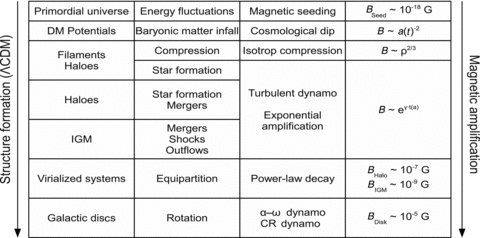
Overview of the different physical processes during structure formation. This table shows the stages of the evolution (column 1), during which an astrophysical process (column 2) triggers an MHD mechanism (column 3) operating on the magnetic field, resulting in the equations and magnetic field strength values given in column 4.
Fig. 3 shows the projected number density of the gas at three different redshifts in the simulation ga2_bx18, together with the corresponding virial radii of the forming galactic halo. Fig. 4 shows the corresponding projected total magnetic field strength, as well as arrows indicating the direction of the magnetic field. The different phases during the formation of the halo and the magnetic field amplification can clearly be seen. The magnetic field agglomerates together with the gas in filaments and protohaloes, where small-scale dynamo action is taking place. Furthermore, as merger events take place, shockwaves are propagating into the IGM creating turbulence. The IGM magnetic field is amplified in stages with several shockwaves propagating into it. Within each shockwave, the magnetic field is possibly amplified by compression within the shockfront and by small-scale dynamo action behind the shockfront (see Kotarba et al. 2011 for an analysis of shockwaves and their effect on the magnetic field during merger events). At a redshift of ≈1, the last major merger event takes place and the magnetic field saturates, i.e. it evolves into energy density equipartition. The magnetic field saturates inside the halo at a mean value of ≈10−7 G and within the IGM at ≈10−9 G, both at redshift 0.
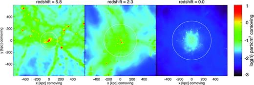
Projected number density ngas in comoving units at different redshifts in the simulation ga2_bx18. The shown regions are cubes with 1-Mpc (comoving) edge length centred on the halo centre of mass. The white circles indicate the virial radius of the halo. The formation of filaments and protohaloes with subsequent merger events can be seen.
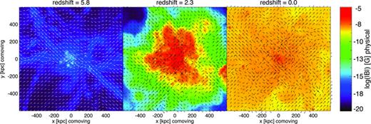
Projected total magnetic field strength and magnetic field vectors in physical units at different redshifts in the simulation ga2_bx18. The shown regions are cubes with 1-Mpc (comoving) edge length centred on the halo centre of mass. Clumping of the magnetic field together with the gas in filaments and amplification within protohaloes can be seen. Furthermore, shockwaves are driven into the IGM increasing the magnetic field strength, until it saturates on all scales.
Fig. 5 shows the rms magnetic field strength inside the galactic halo as a function of redshift for different seed field strengths. The amplification time-scale [i.e. the gradient of the B (a) function during the exponential amplification phase] is the same for all seed fields and only the total time until saturation varies. After saturation, the magnetic field strength decreases with a power-law slope of ≈−1, as irregularities in the magnetic field are dissipated.
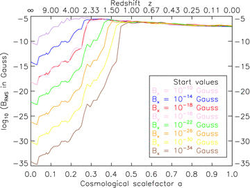
Growth curves of the volume-weighted rms magnetic field strength inside the halo in the simulations GA0 for different seed fields.
Fig. 6 shows radial profiles of the volume-weighted magnetic field strength inside the galactic halo for two different redshifts. At redshift 1 (after the last major merger), magnetic field strengths of several 10−5 G are reached in the centre of the halo and drop to ≈10−7 G at the virial radius with a slope of ≈−1.1. At redshift 0 (virialized system with decaying turbulence), magnetic field strengths of several 10−6 G are reached in the centre of the halo and drop to ≈10−9 at the virial radius with a slope of ≈−0.9. Since the gas density scales linearly with the distance from the galactic halo centre, this indicates a relation of the form B∼ρ.
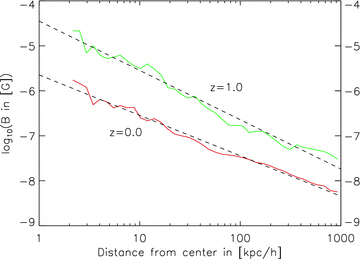
Radial profiles of the mean magnetic field strength inside the halo in the simulation ga2_bx18 for redshifts 1 and 0, respectively. For z= 1, which is just after the last major merger event, the field strength decreases with a slope of −1.1. For the relaxed system at z= 0 the slope is −0.9.
Summing up, within the simulations presented it is possible to amplify a weak primordial magnetic field up to the observed equipartition values.
5.2 Pressures and star formation
Fig. 7 summarizes the energy flow and its effect on the star formation within the simulations. Via internal energy, star formation provides a sink (cooling) and source (supernova injection) of internal energy of the gas. Internal and kinetic energies are mutually exchanging via pressure forces and viscosity. Additionally, the gravitational collapse transforms potential energy into kinetic energy, which is converted partly back into potential energy through the fluid motions in the potential wells. Furthermore, kinetic motions create magnetic energy (induction equation). The Lorentz force describes the back-reaction of the magnetic field on the velocity field. Non-ideal resistivity redistributes the magnetic energy and also converts it into internal energy. Internal, kinetic and magnetic energy densities contribute to a total pressure. The balance between the gravitational collapse and the total pressure support regulates the star formation rate.
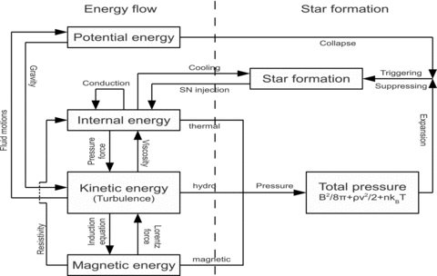
Diagram visualizing the flow of energy in the simulated MHD system. The star formation model provides a source (supernova injection) and a sink (cooling) of energy. On the other hand, the different pressure components (thermal, hydrodynamic and magnetic pressure) have an effect on the star formation.
Fig. 8 shows the magnetic energy density  , the kinetic energy density ɛkin=ρv2/2, the thermal energy density ɛtherm= (γ− 1)ρu and the turbulent energy density
  in the simulation ga2_bx18. The adiabatic index γ is 5/3 and u denotes the internal energy. Similar to Kotarba et al. (2010), vturb is taken as an estimate of the turbulent velocity within the volume defined by an spmhd particle. They find it to be a good spmhd approximation of the turbulent velocity, although it overestimates the turbulence on small scales and ignores the turbulence on scales larger than the smoothing scale.
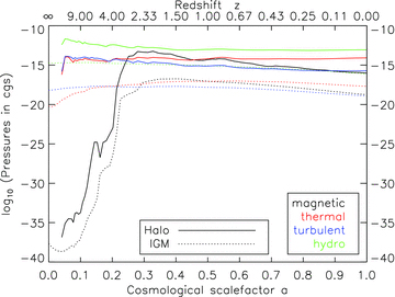
Volume-weighted energy densities as a function of redshift in the simulation ga2_bx18 inside the halo and within the IGM. The magnetic energy density (black line) gets amplified during the phase of halo formation until it reaches equipartition with the other energy densities, particularly the turbulent energy density (blue line).
As shown in Fig. 8, the magnetic energy density increases from the seed value up to equipartition with the turbulent and thermal energy densities until a redshift of ≈3. The cosmological dip can be clearly seen at the start of the simulations. The magnetic energy density overshoots the turbulent energy density slightly in the beginning, which results from possible further compression after equipartition is reached. Afterwards, the virialized system relaxes, and the turbulent and magnetic energies decline. The thermal energy density still rises, as the magnetic and turbulent energies are converted into thermal energy by resistivity and viscosity. With some delay, equipartition is also reached in the IGM by a stepwise amplification process. First, the magnetic field is amplified inside the most dense structures, and subsequently the IGM magnetic field undergoes merger-driven shock amplification.
Fig. 9 shows the total star formation rate as a function of the cosmological scalefactor for all GA0 simulations (see Table 4) with different seed field strengths. Before the formation of filaments and protohaloes, no star formation takes place. At the time the first structures reach the necessary critical density (z≈ 10), star formation begins. As more gas is accreted on to the main halo through gravitational infall or due to merger events, the star formation rate rises. At a redshift of ≈3 it peaks and then starts to decline. For the simulations without any magnetic fields, star formation is still constantly ongoing at a low rate by the end of the simulations. For the simulations including magnetic fields, the star formation rate decreases earlier than in the non-magnetized comparison runs, as soon as equipartition is reached (z≈ 3), and is thus comparatively lower than in the comparison run or even stops completely by the end of the simulations. The magnetic configuration at equipartition provides additional support against further gas accretion, preventing the gas inside the halo from reaching the threshold density necessary to form stars.
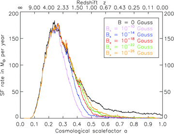
Total star formation rate as a function of redshift in the simulations GA0 with different magnetic seed field. For simulations with magnetic fields, the star formation rate decreases when equipartition is reached and the additional magnetic pressure prevents the gas from reaching the density threshold required for star formation.
Note that the details of star formation depend on the resolution of the simulation. Springel & Hernquist (2003b) show that when increasing the resolution of the simulation, the time when the first stars form is pushed towards higher redshifts. Nevertheless, at low redshifts, the star formation rate converges to a value independent of the resolution. Furthermore, the total stellar mass formed does not change with resolution. These details in the star formation model also influence the turbulent dynamo action. The starting point of the dynamo action depends strongly on the time when the first gas has collapsed, cooled and reached small enough spatial scales. As soon as star formation sets in, additional supernova energy is injected into the system, leading to more turbulence and higher magnetic field growth rates. The saturation value of the magnetic field strength depends on the turbulent energy density, which in turn depends on the total injected feedback, and hence the total stellar mass formed.
The simulation ga1_bx18_nosf (not shown) is performed with the same set-up and methods, but with disabled star formation module. Within this simulation, the magnetic energy density does not get amplified up to equipartition with the turbulent energy density, but only rises a few orders of magnitude. This is clearly because radiative cooling lowers the internal energy of the gas, thus allowing the gas to clump more heavily and reach higher densities. This results in smaller spmhd smoothing lengths, and hence the small-scale dynamo will also operate on smaller scales, thus leading to higher growth rates. Summing up, radiative cooling and supernova feedback are important in MHD simulations of galactic halo formation.
5.3 Numerical reliability
 is a common measure regarding the reliability of spmhd simulations (e.g. Price 2012). It is calculated for every particle i inside its kernel, which is a sphere with radius equal to the smoothing length hi. Even for simulations employing the Euler potentials, which are free of physical divergence by construction, this measure can reach values of the order of unity (Kotarba et al. 2009). The numerical divergence can be regarded as a measure for quality of the numerical calculations and the irregularity of the magnetic field inside each kernel and is not related to possible physical divergence (Kotarba et al. 2010; Bürzle et al. 2011a). Here, an estimator for the numerical divergence of the form
Fig. 10 shows the mean numerical divergence within the halo (solid line) and within the IGM (dashed line) as a function of scalefactor for the simulation ga2_bx18. Throughout the entire simulation, the numerical divergence remains below unity. The numerical divergence is zero in the beginning of the simulations, as expected for a uniform magnetic seed field. During the phases of merger events and magnetic field amplification, the error estimator rises. The turbulent dynamo tangles the magnetic field lines and also creates irregularities below smoothing scales, resulting in a non-vanishing numerical divergence. During the phase of relaxation of the halo, NumDivB decreases, as the field lines are unfolded and ordered and the magnetic energy is dissipated or transferred to larger scales. Within the IGM, the numerical divergence remains constant. This is because within the IGM the NumDivB-decreasing process of magnetic field reordering is balanced by NumDivB-increasing processes. These are the accretion of gas on to the halo and the expansion of space, both resulting in an increasing smoothing length and thus an increasing NumDivB.
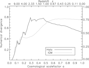
Mean numerical magnetic divergence measure  in ga2_bx18 inside the halo and within the IGM.
6 AGREEMENT OF MODEL AND SIMULATIONS
Since the simulations start at a finite redshift and not at z=∞, a simple shift of  for the initial magnetic field strength in equation (18) is used. The characteristic turbulent quantities in equation (14) are assumed to be constant in space and time. This approximation is good for the phase of strong star formation between redshifts 10 and 1, where the majority of the magnetic amplification is also taking place, while later the growth rate is truncated, and the form of the turbulent quantities is negligible.
In Fig. 11 simulated growth curves of the magnetic field strength are shown (dashed lines). These curves match notably well with the calculated curves (solid lines). Table 2 shows the numerical values used for the calculations, which are resulting in a time-scale (e-folding time) of ≈90 Myr for the growth of the large-scale magnetic field. Extracting such values directly from the simulations is quite challenging, as the density, velocity and length scales within the simulated galactic haloes range over many orders of magnitude. However, the length scale  on which the magnetic energy density increases first within the main halo is determined by the size of star-forming regions, which (within the main halo) can be associated with substructures. Such substructures (clumps of gas, stars and dark matter) can be identified using subfind (Springel et al. 2001a; Dolag et al. 2009). Only the largest substructures still contain gas and form stars within the main halo, having masses of ≈(108–1010) M⊙ and thereby diameters of a few 10 kpc. They are orbiting with typical velocities of a few 100 km s−1, inducing gas rms velocities within the main halo between 50 and 100 km s−1 during the time of rapid growth of the halo, where the magnetic amplification is also taking place (between z≈ 10 and ≈1). Such values strongly motivate the choice of lturb≈ 25 kpc and vturb≈ 75 km s−1, leading to the good agreement between the simulations and the analytical model.

Analytical growth functions (solid lines) as given by equation (18) using the parameters listed in Table 2 for different magnetic seed field strengths. After an initial cosmological dip, the magnetic field grows exponentially until it reaches equipartition with the turbulent energy density. Additionally, the simulated growth curves from Fig. 5 are shown (dashed lines).
Fig. 12 shows a comparison of the analytical growth function (red line) as calculated according to equation 18 using the values given in Table 2 together with the halo rms magnetic field strength in the simulations ga0_bx18, ga1_bx18 and ga2_bx18, respectively. All curves start with the same magnetic seed field of Bstart= 10−18 G. The resolution of the simulations increases by each a factor of roughly 10 from ga0 to ga1 and from ga1 to ga2, respectively. Compared to the simulation with the standard resolution (brown line), the analytical growth function fits the simulated magnetic field evolution very well. Also, for higher resolutions (black and green lines), the fit is convincing. Note that for higher resolutions, star formation sets in at higher redshifts, leading to an earlier rise of collapsed, cooled gas and feedback and hence an earlier starting point for the turbulent dynamo. Nevertheless, the saturation value of the magnetic field strength is indistinguishable.
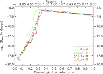
Volume-weighted rms magnetic field strength inside the halo as a function of redshift for three simulations with the same magnetic seed field of 10−18 G but different resolution, together with the analytical growth function (see equation 18 and Table 2). The analytical function fits the simulated evolution of the halo magnetic field very well.
For the calculation of the hydrodynamic and magnetic Reynolds numbers, the typical velocity V and length scale L are determined by the physical properties of the system, i.e. the sound speed  and the Alfvén speed
  , and the size of the halo, respectively, which do not depend on resolution. Within all the simulations, a constant turbulent resistivity ηturb is used, and hence Rm stays constant. Additionally, artificial viscosity as given by Price (2012) is applied, where ν depends on particle properties and spacings. A higher resolution thus leads to smaller ν, and thus (given the constant V and L) to higher Re numbers and hence more turbulence. A higher (or, better resolved) turbulence in turn results in a higher growth rate of the magnetic field.
The cosmological turbulent dynamo as described by equation (18) reproduces the main features of the simulated non-ideal magnetic field amplification very well.
7 SUMMARY
In this paper, the evolution of magnetic fields during galactic halo formation is discussed. The main focus is placed on the investigation of the processes responsible for the amplification of magnetic fields from seed field levels to observed values. An analytical model for the evolution of the magnetic field driven by a turbulent dynamo is presented and the predictions of this model are compared with numerical, cosmological simulations of Milky Way-like galactic halo formation including the evolution of magnetic fields, radiative cooling and star formation. The most important results are summarized as follows.
A primordial magnetic seed field of low strength can be amplified up to equipartition with other energy densities during the formation and virialization of a galactic halo in a ΛCDM universe. The final magnetic field strength decreases with a slope of ≈−1.0 from ≈10−6 G in the centre to ≈10−9 G behind the virial radius (IGM) of the halo and also reaches ≈10−5 G in interacting systems. These values are in notably good agreement with observations (Beck et al. 1996; Kronberg et al. 2008).
The magnetic field amplification in filaments and protohaloes is dominated by turbulent dynamo action. Radiative cooling of the primordial gas is needed in order to reach spatial scales small enough for the turbulent dynamo to operate efficiently. Equipartition is reached on small scales first and later on larger scales, consistent with theoretical expectations (Brandenburg & Subramanian 2005; Shukurov 2007; Arshakian et al. 2009). The turbulence is driven by the gravitational collapse, by supernova activity and by mergers of protohaloes into the main galactic halo. After equipartition is reached, the magnetic energy decays with a power-law dependence of Bt∼t−4/3. The IGM magnetic field is amplified by outflows of magnetized gas from the centre of the haloes and by merger-driven shock amplification outside the main halo.
The amplification time-scale (e-folding time) of the order of 107 yr is small enough to describe the generation of strong magnetic fields in irregular galaxies at high redshifts as observed (e.g. Bernet et al. 2008).
The structure of the resulting magnetic field is random and turbulent. Additional dynamo processes, e.g. the α–ω dynamo (Ruzmaikin et al. 1979; Shukurov 2007) or the cosmic ray-driven dynamo (Lesch & Hanasz 2003; Hanasz et al. 2009), are needed to produce regularity in the magnetic field topology.
Last, but not least, a basic analytical model is able to reconstruct the numerical results very accurately. Weak magnetic perturbations grow in a non-stationary turbulent hydrodynamical flow. This amplification is slightly modified by the ΛCDM cosmology, particularly in the early universe. Non-ideal truncation of the growth rate finally yields equipartition. These processes result in an analytical growth function which fits the simulations astonishingly well.
In the current picture of galaxy formation – together with cooling and star formation – magnetic fields are efficiently amplified from seed field levels up to the observed values. However, their detailed influence on the dynamics of the gas and the underlying seeding mechanisms still remains unclear and needs to be investigated further.
We thank the anonymous referee for the comments, which helped to improve many parts of this paper. Special thanks to Felix Stoehr for providing the original initial conditions. Rendered graphics are created with P-smac2 (Donnert et al., in preparation). FAS is supported by the DFG Research Unit 1254. KD is supported by the DFG Priority Programme 1177 and by the DFG Cluster of Excellence ‘Origin and Structure of the Universe’.
REFERENCES
