


Abstract
We compare the semi-analytic models of galaxy formation of Fu et al. which track the evolution of the radial profiles of atomic and molecular gas in galaxies, with gas fraction scaling relations derived from a stellar mass-limited sample of 299 galaxies from the CO Legacy Database for GASS. These galaxies have measurements of the CO(1–0) line from the IRAM 30-m telescope and the H i line from Arecibo, as well as measurements of star formation rates, stellar masses, galaxy sizes and concentration parameters from GALEX+SDSS photometry. The models provide a good description of how condensed baryons in star-forming galaxies are partitioned into atomic and molecular gas and stars as a function of galaxy stellar mass and stellar surface density. The models do not reproduce the observed tight relation between stellar surface mass density and bulge-to-disc ratio in these galaxies. The current implementation of ‘radio-mode feedback’ in the models produces trends that disagree strongly with the data. In the models, gas cooling shuts down in nearly all galaxies in dark matter haloes above a mass of ∼1012 M⊙. As a result, stellar mass is the observable that best predicts whether a galaxy has little or no neutral gas, that is, whether a galaxy has been quenched. In contrast, our data show that quenching is largely independent of stellar mass. Instead, there are clear thresholds in bulge-to-disc ratio and in stellar surface density that demarcate the location of quenched galaxies in our chosen parameter space. We speculate that the disagreement between the models and the observations may be resolved if radial transport of gas from the outer disc is included as an additional bulge formation mechanism in the models. In addition, we propose that processes associated with bulge formation play a key role in depleting the neutral gas in galaxies and that gas accretion is suppressed in a significant fraction of galaxies following the formation of the bulge, even in dark matter haloes of low mass.
1 INTRODUCTION
An important goal in modern galaxy formation is an improved understanding of the physical processes that regulate the rate at which stars form in galaxies. These processes include the cooling and accretion of gas within dark matter haloes, the transformation of the accreted gas into molecular clouds and stars, and the effects of ‘feedback’ from massive stars and accreting black holes on to the gas in and around galaxies.
The Λ cold dark matter (ΛCDM) model provides detailed predictions for how dark matter haloes assemble over time. Within these haloes, gas will cool and settle into a rotationally supported disc. One hotly debated issue is the degree to which gas loses angular momentum to the surrounding dark matter during this process. In many ‘semi-analytic’ models, the angular momentum of the gas is assumed to be conserved. This produces a size–circular velocity relation for galactic discs that is in good agreement with observations (Mo, Mao & White 1998). More detailed numerical hydrodynamical simulations of disc galaxy formation in a ΛCDM universe demonstrate, however, that the amount of angular momentum that is lost during the collapse of the dark matter halo depends sensitively on how feedback processes are included in the models (Navarro & Steinmetz 1997; Governato et al. 2004, 2007). In many simulations, the discs form early and are too compact. The resulting star formation time-scales are then too short to be consistent with observations (e.g. Oser et al. 2010).
Another important unsolved problem is to understand why galaxies divide into two distinct ‘families’– those with ongoing active star formation and those where star formation has been quenched (Strateva et al. 2001; Kauffmann et al. 2003b; Baldry et al. 2004). It has now become clear that these distinctions existed already at redshifts as high as 2.5 (Williams et al. 2010; Wuyts et al. 2011), when cold gas accretion rates in almost all dark matter haloes are predicted to be very high.
Many recent theoretical galaxy formation models that aim to reproduce the statistical properties of the massive galaxy population (e.g. Bower et al. 2006; Cattaneo et al. 2006; Croton et al. 2006; De Lucia & Blaizot 2007; Somerville et al. 2008; Guo et al. 2011; Lu et al. 2011) invoke star formation quenching mechanisms that set in at a characteristic dark matter halo mass. The characteristic mass is associated with the transition between the regime where gas cooling times are short compared to the dynamical time of the dark matter halo and gas accretes in the form of cold, condensed clouds, and the regime where cooling times are long and gas accretes from a corona of gas that is in virial equilibrium with the surrounding halo.
One might ask why lowered rates of star formation in galaxies should be linked with this transition. One argument that is often used is that relativistic jets, generated when gas accretes on to black holes, heat the surrounding hot gas and prevent it from forming stars (see e.g. Croton et al. 2006). The conditions under which black holes produce jets are not well understood. There is clear observational evidence that radio-emitting jets play a role in regulating the cooling of gas in nearby galaxy clusters (see McNamara & Nulsen 2007, for a recent review). Theoreticians have thus made an ‘ansatz’ that jets from radio-loud active galactic nuclei (AGNs) will prevent gas from cooling and forming stars in all dark matter haloes that are predicted to contain a hot gas atmosphere. The characteristic halo mass threshold that separates star-forming and quiescent galaxies is the main factor that determines how massive galaxies evolve in current models, so it is clearly important to test the existence of such a threshold using real observations.
We note that accretion and quenching processes affect the gas components of galaxies. The most direct empirical constraints on how they operate thus come from observations of the gas in galaxies. This has been the primary motivation for the GALEX Arecibo SDSS Survey (GASS), as well as the CO Legacy Database for GASS (COLD GASS), which is measuring the atomic and molecular gas contents of an unbiased sample of several hundred galaxies with redshifts between 0.025 and 0.05, and with stellar masses in the range 1010 < M* < 1011.5 M⊙. In both surveys, the strategy is to observe each galaxy until the H i/CO lines are detected, or until upper limits in the ratio of atomic and molecular gas mass to stellar mass of ∼0.015 reached. The aim of the programme is to carry out a census of the condensed baryons in galaxies in the local Universe, to study scaling relations between the gas and stellar properties of these galaxies, and to understand gas accretion and quenching in galaxies.
Details of the GASS and COLD GASS designs, as well as target selection and observing procedures, are given in Catinella et al. (2010) and Saintonge et al. (2011a). These two papers also presented relations between the H i and H2 mass fractions of galaxies (defined as MH I/M* and  ) and global galaxy parameters such as stellar mass M*, stellar mass surface density μ*, galaxy bulge-to-disc ratio (as parametrized by the concentration index C of the r-band light), and specific star formation rate sSFR = SFR/M* (see also Schiminovich et al. 2010). The two surveys uncovered sharp thresholds in μ* and C below which all galaxies have a measurable cold gas component, but above which the detection rate of the CO and H i lines drops suddenly, suggesting that ‘quenching processes’ have occurred in these systems.
In this paper, we compare the observed gas fraction relations from COLD GASS with predictions from the semi-analytic models of Fu et al. (2010, hereafter F10) which track the formation of molecular gas in disc galaxies. The F10 models are based on the L-Galaxies semi-analytic code, described in detail in Croton et al. (2006) and updated in De Lucia & Blaizot (2007).
The models are currently being configured to operate on the latest update of the L-Galaxies code by Guo et al. (2011); the comparison in this paper will be restricted to the version of the models in F10. The main new aspect of these models is that galactic discs are represented by a series of concentric rings in order to track the evolution in the gas and stellar surface density profiles of galaxies over cosmic time. Two simple prescriptions for molecular gas formation processes are included: one is based on the analytic calculations by Krumholz, McKee & Tumlinson (2009, hereafter KMT), and the other is a prescription where the H2 fraction is determined by the pressure of the interstellar medium (Blitz & Rosolowsky 2006, hereafter BR), with an implementation similar to that in Obreschkow et al. (2009). The free parameters of the models that regulate the rate at which gas is turned into stars and the efficiency with which supernovae reheat gas as a function of halo mass have been tuned to reproduce a number of key observables, including the observed present-day galaxy luminosity function, the gas-phase mass–metallicity relation, and the mean H i gas fraction as a function of B-band luminosity (see De Lucia, Kauffmann & White 2004, for a more detailed discussion).
There have been a number of other cosmological models that follow the formation of molecular gas in discs. Lagos et al. (2011) have developed semi-analytic models that track molecular gas formation in cosmological simulations of galaxy formation, but these models do not predict the detailed radial profiles of galaxies as in F10. Robertson & Kravtsov (2008) and Dutton, van den Bosch & Dekel (2010) model the radial profiles of the gas and stars in galaxies, but their models are not embedded within full cosmological N-body simulations. Gnedin, Tassis & Kravtsov (2009) have carried out very high resolution cosmological simulations of molecular gas formation which include radiative transfer and detailed treatment of the chemistry, but their box sizes are too small to make statistical predictions.
F10 demonstrated that their models could fit the radial H i, H2, stellar mass and SFR profiles of spiral galaxies from THINGS/HERACLES. In this paper, we investigate whether the models also yield correct gas fraction scaling relations and distribution functions. As will be seen, it is useful to break this analysis into two distinct parts: (1) comparison between models and observations of the distribution of gas fractions in the population of galaxies with detectable gas; and (2) comparison of how absence of gas, which we refer to as ‘quenching’, is manifested as a function of observable quantities such as stellar mass, stellar surface density and bulge-to-disc ratio. As we will show, such a comparison elucidates those aspects of the models that work well, and those that fail. Throughout this paper, we have assumed a cosmology with Ω= 0.3, Λ= 0.7 and H0= 70 km s−1 Mpc−1 to derive our observational quantities. The cosmology assumed for the F10 model is a ΛCDM model with Ω= 0.25, Λ= 0.75, H0= 73 km s−1 Mpc−1 and σ8= 0.9.
2 GENERATING COMPARISON SAMPLES FROM THE SIMULATIONS
The semi-analytic models used in this paper are nearly identical to those described in detail in F10. We have made only one small change. The free parameters in the F10 models were chosen so that reasonable fits to a variety of observables could be obtained. These observables included the H2 mass function of Keres, Yun & Young (2003) derived using galaxies drawn from the FCRAO Extragalactic CO Survey (Young et al. 1995). These authors adopted a CO-to-H2 conversion factor that was a factor of 1.5 times larger than the one adopted by Saintonge et al. (2011a).1 To bring the simulations back into agreement with the H2 data using the conversion factor adopted by Saintonge et al., we simply increase the supernova reheating rate (given by the parameter εdisc) in table 1 of F10 by a similar factor (εdisc= 5 instead of 3.5). We note that changing εdisc simply shifts the amplitude of the gas mass fraction scaling relations up or down. It does not change the predicted slope or scatter in these relations. We also note that the H2 mass function derived from the COLD GASS data for galaxies with log M* > 1010 M⊙ agrees well with that of Keres et al. (2003) at the high-mass end, once the same CO-to-H2 conversion factor is adopted (Fu et al., in preparation).
The observational sample is an update to that described in Saintonge et al. (2011a), consisting of 299 galaxies with CO(1–0) line observations with the IRAM 30-m telescope. H i line measurements from GASS (Catinella et al. 2010) are available for 270 out of the 299 galaxies. Because the observational sample is selected only by stellar mass, it is easy to compare simulation results directly with the data. There are only two observational selection issues that require careful treatment:
In both GASS and COLD GASS, targets are selected so that the resulting stellar mass distribution is approximately flat. This was done in order to be able to compute gas fractions in different stellar mass bins with roughly the same errors. The sampling must be taken into account when we look at gas fraction distributions as a function of parameters other than stellar mass. In this paper, we adopt two approaches: (a) we weight each galaxy in the sample by the inverse of f(M*), where f(M*) is the ‘sampling rate function’ required to transform the true stellar mass distribution to a flat one; or (b) we apply the sampling rate function f(M*) to the simulated galaxies to create a ‘mock catalogue’ with flat stellar mass distributions that can be compared directly with the data.
It is important to take account of the detection limits of the survey when comparing model galaxies with the data. This is illustrated in the top panels of Fig. 1, where we plot
 (top left-hand panel) and M(H2)/M* (top right-hand panel) as a function of stellar mass for 299 galaxies that have been observed in CO as of 2011 July (270 of these have H i observations from GASS). Galaxies where the H i or CO line was detected (see Catinella et al. 2010; Saintonge et al. 2011a, for details about line-detection procedures) are plotted in blue. Galaxies without detections are plotted in red at the positions of their 5σ upper limits in
  or M(H2)/M*.
To a very close approximation, the H i mass fraction limit, log [ M(H I)/M*]lim, is −1.82 (corresponding to a H i mass fraction limit of 0.015) for galaxies with log M* > 10.3. For galaxies with 10 < log M* < 10.3, log [ M(H I)/M*]lim=− 1.066 log M*+ 9.16.
The CO line-detection limits are somewhat more complicated. As discussed in Saintonge et al. (2011a), the integration times are set so that log [M(H2)/M*]lim=−1.82 for galaxies with log M* > 10.6. For lower mass galaxies, integration times are nominally set to reach a fixed rms of around 1.1 mK per 20 km s−1 wide channel, but the actual value fluctuated according to weather conditions at the time of observation. Therefore, when creating our mock catalogues from the simulations, we simply impose a distribution of upper limits similar to that seen in the top right-hand panel of Fig. 1. We take [M(H2)/M*]lim, max, the maximum possible value of the H2 mass fraction limit, as log [M(H2)/M*]lim, max=−1.72 if log M* > 10.6, and log [M(H2)/M*]lim, max= 8.78 − log M* if log M* < 10.6. The H2 mass fraction limit that we adopt is randomly distributed between the maximum value and a minimum value that is 0.35 dex smaller.
![In the left-hand panels, H i mass fraction [log M(H I)/M*] and sSFR (log SFR/M*) are plotted as a function of log M*. The blue points denote galaxies with H i line detections. The red points denote galaxies where H i was not detected. In the right-hand panels, H2 mass fraction [log M(H2)/M*] and sSFR (log SFR/M*) are plotted as a function of log M*. The blue points denote galaxies with CO line detections. The red points denote galaxies where CO was not detected.](https://oup.silverchair-cdn.com/oup/backfile/Content_public/Journal/mnras/422/2/10.1111/j.1365-2966.2012.20672.x/2/m_mnras0422-0997-f1.jpeg?Expires=1750182052&Signature=b0L9WorWX3BXiv9bp56uzIHeCC-25EQD6CZ66YlzMfwMr9FahnuOMVzcca3Rst3QLV58mhWS5CJUwcC2f-wqlbSfRmetAAGjqPrMl8Pp0wc080qONvUrpfL5fwsskcNtmAvvvPYvX6TNm68nYgQlaZOYtJsDWhlicgHWTvkLpodTLOprJd~C9uvb8azWygg2pwYfPzVbSXAcmwbLGcq4Tw0AYygBfBqWUSqX5euPTkYoWRXYCFeXa8M854RTZkUN2ylecdxwi5jnSMsy4BU01gFL4IAPEg4vrSqX0yR9c5Q6LIVyHCsUMFtWsNe3G06c2iNAIFgJvyZN3OX1i4NVgQ__&Key-Pair-Id=APKAIE5G5CRDK6RD3PGA)
In the left-hand panels, H i mass fraction [log M(H I)/M*] and sSFR (log SFR/M*) are plotted as a function of log M*. The blue points denote galaxies with H i line detections. The red points denote galaxies where H i was not detected. In the right-hand panels, H2 mass fraction [log M(H2)/M*] and sSFR (log SFR/M*) are plotted as a function of log M*. The blue points denote galaxies with CO line detections. The red points denote galaxies where CO was not detected.
In this way, we are able to classify galaxies in the simulations as H i/CO ‘detections’ or ‘non-detections’ and compare properties such as stellar masses, stellar surface densities, sSFRs and concentration indices with those of the real galaxies in our survey. We note that stellar masses and SFRs are standard outputs of semi-analytic models. Because the F10 models are able to track radial profiles of the gas and stars in galaxies, they are also able to predict stellar surface mass densities which are defined as  , where R50 is the radius containing half the stellar mass of the galaxy.
In semi-analytic models, bulges form either as a result of a merger between two galaxies, or as a consequence of instabilities that set in when discs reach a certain critical threshold density. In the models, the total mass of the bulge is more reliably predicted than its size. As shown in fig. 1 of Weinmann et al. (2009), there is a tight correlation between the concentration index C (defined as the ratio of the radii containing 90 and 50 per cent of the r-band light) and galaxy bulge-to-disc radio derived using two-dimensional decomposition codes (Gadotti 2009). We have therefore elected to transform the bulge-to-disc ratios predicted by the models to concentration indices using a fit to this relation: C= 1.8 + 2.14B/T.
3 RESULTS
In the analysis presented in this paper, we will attempt to answer the following two questions:
Can the simple disc formation models described in F10 explain observed gas fraction scaling relations for galaxies with gas?
Does the transition between the population of galaxies with gas and the population without gas occur in the same way in the models and in the data?
We have chosen the gas fraction detection threshold of our two surveys as the nominal division between the population of galaxies we will henceforth refer to as ‘active’ and the population that we will call ‘quenched’. Note that it is possible that some fraction of galaxies classified as ‘active’ are actually losing their gas and evolving into quenched systems. Conversely, some fraction of galaxies classified as ‘quenched’ may have simply run out of gas just prior to the next accretion episode. Such galaxies may be thought of as ‘transition’ systems.
In the bottom panels of Fig. 1, we plot sSFR versus stellar mass for the galaxies in our sample. In the bottom left-hand panel, galaxies with H i detections are colour-coded in blue and those where the H i line was not detected are colour-coded in red. In the bottom right-hand panel, we do the same thing according to whether the CO line was detected or not. As can be seen, galaxies with log SFR/M* < −11 are not usually detected in H i and almost never in CO. This means that there is a rather clean distinction between ‘active’ and ‘quenched’ galaxies which applies to both gas fraction and sSFR for the majority of galaxies in our sample. In Section 3.2.2, we return to the issue of whether we can identify a subpopulation of galaxies that are in the process of being quenched.
3.1 Gas scaling relations for the active population
In Figs 2 and 3, we compare the mean H i and H2 gas fractions as a function of M*, μ*, C and SFR/M* for data and for models. The reader is referred to Catinella et al. (2010) and Saintonge et al. (2011a) for details on how H i and CO line fluxes are transformed into H i and H2 masses. We note that we have adopted a constant Galactic conversion factor αCO= 3.2 M⊙ (K km s−1 pc2)−1 which does not include a correction for the presence of helium. A constant conversion factor should be a reasonable approximation for the galaxies in our survey which all have stellar masses greater than 1010 M⊙ and gas-phase metallicities near solar (Saintonge et al. 2011b).
![The mean H i mass fraction [log M(H I)/M*] for COLD GASS galaxies with H i line detections (blue points) is plotted as a function of stellar mass, stellar mass surface density, concentration and sSFR. Error bars are calculated using bootstrap resampling. Results for the F10 models are shown as the black (KMT atomic-to-molecular gas prescription) and red (BR pressure prescription) curves.](https://oup.silverchair-cdn.com/oup/backfile/Content_public/Journal/mnras/422/2/10.1111/j.1365-2966.2012.20672.x/2/m_mnras0422-0997-f2.jpeg?Expires=1750182052&Signature=rAufz~9RfxXJ5RZBi~2RVNyQVeUsMYipVyCQ-x1N9VRUXpYmSS33T9hM~V9R8CplxjvD36fENkj-bNPRSzxV2Ai9O4cjROMFN2kjGsjyK4yNUcK3kUu77OX1T8JNkkH-hPf49Cqhoxcu-gSXc0OChUJihnYU70dK1YGTDNa2ERbHKgQhtRfwMbvSNzBmUSYGCcQyKlWZoJbMYX45A1cfIKz-NyC6sX0DK9UZTXE0Crmktyh3at7IdsjKAx7n1e-nDl1QuU8cFERz~Uu7LOZaiAFCyhE7p3tbxhKQ1riz92yUciaYPkFF62fGKu-2g34CS8w7NJrc595j1yE8yCkw5w__&Key-Pair-Id=APKAIE5G5CRDK6RD3PGA)
The mean H i mass fraction [log M(H I)/M*] for COLD GASS galaxies with H i line detections (blue points) is plotted as a function of stellar mass, stellar mass surface density, concentration and sSFR. Error bars are calculated using bootstrap resampling. Results for the F10 models are shown as the black (KMT atomic-to-molecular gas prescription) and red (BR pressure prescription) curves.
![The mean H2 mass fraction [log M(H2)/M*] for COLD GASS galaxies with CO line detections (blue points) is plotted as a function of stellar mass, stellar mass surface density, concentration and sSFR. Error bars are calculated using bootstrap resampling. Results for the F10 models are shown as the black (KMT atomic-to-molecular gas prescription) and red (BR pressure prescription) curves.](https://oup.silverchair-cdn.com/oup/backfile/Content_public/Journal/mnras/422/2/10.1111/j.1365-2966.2012.20672.x/2/m_mnras0422-0997-f3.jpeg?Expires=1750182052&Signature=F5eeDq7cnLsQ0mEXaJoe5k0k6MMxqvnGLDOZ0Zf3dUHbca~0P~Fkfb6~~MetoK38bJ9fPmfjdw60iAJuHv~5JnR6xLglMnUQegwhXKrUbW0VPpIA17BhtQfb87lbXjvj7gH96G7n~0QtUtG~keuzhbLYiz~Ele6C3c6wj2XOYzQk~CTUpcvE1L64IWCq5CFLPRUWfU9g0~hviTCcE4EWGMjXw2GbinaIPMFeyKqLyiVmdR7exwoBvUGjOcQ7EIsTd~G~afZ9kL9o6YI5FqjqDCdpIujRNJukYSYBDMihIc3wHbIud6K5dPd6fom0JUn2tcOtUEDjpxO-2Sws36DKsg__&Key-Pair-Id=APKAIE5G5CRDK6RD3PGA)
The mean H2 mass fraction [log M(H2)/M*] for COLD GASS galaxies with CO line detections (blue points) is plotted as a function of stellar mass, stellar mass surface density, concentration and sSFR. Error bars are calculated using bootstrap resampling. Results for the F10 models are shown as the black (KMT atomic-to-molecular gas prescription) and red (BR pressure prescription) curves.
In Figs 2 and 3, the blue points show the mean values of M(H I)/M* and M(H2)/M* calculated using the galaxies with H i and CO line detections. Error bars are calculated using bootstrap resampling. The red and black curves indicate the mean values calculated from the model galaxies that are classified as detections (see Section 2). The black curves show results from the F10 model that uses the KMT prescription for the conversion of atomic to molecular gas. The red curves show results from the F10 model that uses the BR pressure-based prescription. We note that there are many more simulated galaxies than observed galaxies. In generating the curves, we have ordered the galaxies by increasing M*, μ*, C and SFR/M* and computed means for bins of 70 galaxies.
Figs 2 and 3 show that the models reproduce the observed scalings between mean H i/H2 mass fraction and galaxy stellar mass, surface mass density and concentration quite well. The differences between the H i mass fractions predicted by the KMT and BR prescriptions are small. Given the systematic uncertainties in the calibration of the BR prescription, the fact that the KMT prescription is based on simple analytic calculations, the fact that our semi-analytic disc formation models are extremely idealized, and the fact that the model free parameters were not tuned to fit the COLD GASS scaling relations, we find it remarkable how well these results agree with the data.
The relation between H2 mass fraction and sSFR is shallower than predicted by the models, which lie on a relation with slope unity. The discrepancy in the relation between M(H2)/M* and SFR/M* is easily understood in light of the results presented in Saintonge et al. (2011b). The F10 models adopt the assumption that  with α constant (corresponding to an effective molecular gas depletion time-scale of 2 Gyr) in all galaxies. This assumption was motivated by the results in Leroy et al. (2008). Saintonge et al. (2011a) showed, however, that there was more than a factor of 5 variation in the global molecular gas depletion time-scale in different galaxies, and that the least actively star-forming galaxies (i.e lowest values of SFR/M*) had the longest depletion times. This explains the shallow observed relation in the bottom right-hand panel of Fig. 3.
In Fig. 4, we show scatter plots of log SFR/M* versus log M(H2)/M* and log M(H I)/M* for our survey galaxies (blue points) and for galaxies from our mock catalogue (black points). Results are only shown for the KMT atomic-to-molecular gas prescription, because results for the pressure prescription are virtually the same. As can be seen, the models reproduce the scatter in sSFR versus atomic gas fraction quite well, but not in sSFR versus molecular gas fraction. Clearly, there are additional processes at work that determine the rate at which molecular gas will form stars. This is the subject of a future paper (Saintonge et al., in preparation).
![Scatter plots of H2 mass fraction [log M(H2)/M*, left-hand panel] and H i mass fraction [log M(H I)/M*, right-hand panel] for COLD GASS galaxies are shown as the blue points. Results from the F10 models with the KMT atomic-to-molecular gas prescription are shown as the black points.](https://oup.silverchair-cdn.com/oup/backfile/Content_public/Journal/mnras/422/2/10.1111/j.1365-2966.2012.20672.x/2/m_mnras0422-0997-f4.jpeg?Expires=1750182052&Signature=pOq2QJVCWF~h7EczQ1bLQz-L6ayoi-tqDup6rsga2w9qvttCbPbcZOt81CsMtv-CyNXeqUURhlvuJO7jV7RD4mUH6tsy4iOPRAUofStHIZTeV8eFq9MYJRqRid6RX~~O0sRcVK~3V9RCxqzdqmHph201vbzVRT3Pviqf3x3IeGKC0NzZe3fzLd2zk1sBqBRBm5xLQBDwO5YJBDx7ZKnw6Cg7WAuuIoLp1VhnwFHYx36eaNT2WfReDMti8fHReUzvUEnuXjjKIFsHrCdAy4yGQ9k7gYdoNoAu9Zk~qhVb7sH43oOgjAfgDcIoEzceZcgScamgzVaxu7mu4B4quze5qg__&Key-Pair-Id=APKAIE5G5CRDK6RD3PGA)
Scatter plots of H2 mass fraction [log M(H2)/M*, left-hand panel] and H i mass fraction [log M(H I)/M*, right-hand panel] for COLD GASS galaxies are shown as the blue points. Results from the F10 models with the KMT atomic-to-molecular gas prescription are shown as the black points.
As well as looking at mean H i and H2 mass fraction relations for galaxies with detections, it is instructive to analyse full distribution functions of gas mass fractions. These are illustrated in Figs 5 and 6. The data are shown as the blue histograms, with error bars computed from bootstrap resampling. The black and red curves are for the models, as before. We plot distributions of log M(H I)/M* and log M(H2)/M* in three different intervals of stellar mass, stellar mass surface density and concentration. These plots show that the models provide a good representation not only of the mean H i/H2 mass fractions, but also of the scatter around the mean. As discussed in F10 and will be illustrated below, there is a tight relation between stellar mass and dark matter halo mass in the models. The scatter around the mean gas fraction at fixed dark matter halo mass is set by (a) the spin parameter of the halo which determines the contraction factor of the accreted gas and hence the rate at which it will be consumed into stars; and (b) the recent gas accretion history of the galaxy. The fact that the scatter in the models and data agree so well lends support to this basic picture.
![Distribution functions of H i mass fraction [log M(H I)/M*] for COLD GASS galaxies with H i line detections in three ranges of stellar mass, stellar mass surface density and concentration (blue histograms). Error bars are calculated using bootstrap resampling. Results for the F10 models are shown as the black and red curves. The colour-coding of the model curves has the same meaning as in Figs 2 and 3.](https://oup.silverchair-cdn.com/oup/backfile/Content_public/Journal/mnras/422/2/10.1111/j.1365-2966.2012.20672.x/2/m_mnras0422-0997-f5.jpeg?Expires=1750182052&Signature=dqMxywWakkU4Ni~Bsd61dMG9aIlN9eDa0i7lkwvprE~oU6-lLwujCtC6i9Bztx4j24gP~gqI-F2Vis41N-xCF1brVruwIC3G4Z596QJhk4IrvWb9Kke8IK05byg-Xr90MOSJF9V1h7nyuaa8WGtAwdmmhpW2atUYEXVH0iOCc3sWOHph2aNY3rdo3GSix6YWr7XLoMwgEnhZeiFAncTSehp6GKhcjB42LqOYJ7H7X0F4r0nQCVNO~gpyh0L9uqghcoheALuvKvOjd03Ey5K03rsKzbNqxNe7~DTKQaIss18IbGUpWqr0nRa0ojR3Qq5JIokJTtW3D44l8qLcMcBDgg__&Key-Pair-Id=APKAIE5G5CRDK6RD3PGA)
Distribution functions of H i mass fraction [log M(H I)/M*] for COLD GASS galaxies with H i line detections in three ranges of stellar mass, stellar mass surface density and concentration (blue histograms). Error bars are calculated using bootstrap resampling. Results for the F10 models are shown as the black and red curves. The colour-coding of the model curves has the same meaning as in Figs 2 and 3.
![Distribution functions of H2 mass fraction [log M(H2)/M*] for COLD GASS galaxies with CO line detections in three ranges of stellar mass, stellar mass surface density and concentration (blue histograms). Error bars are calculated using bootstrap resampling. Results for the F10 models are shown as the black and red curves. The colour-coding of the model curves has the same meaning as in Figs 2 and 3.](https://oup.silverchair-cdn.com/oup/backfile/Content_public/Journal/mnras/422/2/10.1111/j.1365-2966.2012.20672.x/2/m_mnras0422-0997-f6.jpeg?Expires=1750182052&Signature=X6juX8ZmFIaQ-fc7d1zTbBTCSADjn2mRW3ojcUqJHPvqfDSFavbE2towHBg119aeCfhEEBSVfti4OKwcXqB4U57Gz33Q9Bcp8TGseYSO6dRssjScICNFxWviZoUhZ5R7y2~lZNpOUz8z7w0GDXbJE2UjLzuGa0SGWAyXyvsiDorNa5JbKgsIy1w6kZdS6Vn0~D8Bv7TmC-fiv~WChxg4~lVyAplUye8WGFNLRHv6oOr3G-SXur08-mci9uOhLvSVAwQlWzCJvcgNnjXuuiKDW4Jwf5tiZhEmzHPS-Hx-1jn1MR4eFd8WRq56THSsHgQHdQFItVk45TK1x8mGLmLpJQ__&Key-Pair-Id=APKAIE5G5CRDK6RD3PGA)
Distribution functions of H2 mass fraction [log M(H2)/M*] for COLD GASS galaxies with CO line detections in three ranges of stellar mass, stellar mass surface density and concentration (blue histograms). Error bars are calculated using bootstrap resampling. Results for the F10 models are shown as the black and red curves. The colour-coding of the model curves has the same meaning as in Figs 2 and 3.
We note that in recent years, there have been a number of papers questioning the treatment of disc formation in semi-analytic models (e.g. Sales et al. 2009). The primary objection is the assumption that the angular momentum of a galaxy expressed in units of that of its surrounding halo (jd=Jgal/Jvir) correlates with the mass of the galaxy divided by the mass of its dark matter halo (md=Mgal/Mvir) in a manner that is insensitive to feedback, that is, jd=md is assumed for all haloes. In our scheme, this is not the case. We only assume that jd=md for the gas that is cooling instantaneously at any given time in any given halo. Because we track the growth of galaxies and dark matter haloes with time, and because feedback effects will affect the mass of gas that cools in haloes of different masses at different redshifts, the resulting relation between the angular momentum of the galaxy and its mass fraction will depend on feedback.
Fig. 5 also shows that the models miss a minority population of galaxies with high atomic gas fractions and with low stellar masses, surface mass densities and concentrations. What are these missing galaxies? In three recent papers, we have studied the properties of galaxies in our survey that contain significantly more atomic gas than would be predicted from their UV/optical colours and sizes (Moran et al. 2010; Moran et al. 2012; Wang et al. 2011). The main conclusion is that such galaxies have very blue outer discs with young stellar populations and low gas-phase metallicities. These results led us to propose that these unusually H i rich systems have experienced a recent gas accretion event, resulting in the growth of the outer disc.
In the F10 models, the accreted gas is always added to the disc with an exponential surface density profile. In real galaxies, the accreted gas may initially be distributed in the outer regions of the galaxy. Dynamical perturbations in the form of spiral density waves, interaction with companions or with the non-axisymmetric gravitational potential of the surrounding dark matter halo, will eventually be the cause for the gas to flow inwards and reach high enough densities to form molecular clouds. If we change the gas accretion prescriptions so that accreted gas is initially dumped in the outskirts of the disc, this may produce a tail of H i-rich galaxies. Observations of SFR, metallicity and gas profiles will be required to constrain models of this nature.
3.2 The nature of the quenched population
In this section, we investigate whether the ‘transition’ between the population of galaxies with detectable atomic and molecular gas and the populations with gas fractions below ∼0.015 occurs in the same way in models as in the data. In Figs 7 and 8, we plot the fraction of H i/CO detected galaxies as a function of stellar mass, stellar mass surface density, concentration index and sSFR. Results from the survey are shown as the solid blue lines. The dashed blue lines indicate the ±1σ uncertainty in the detected fraction as a function of these parameters. Model results are shown in red and black (the colour-coding is the same as in Figs 2 and 3). The main conclusion from these two figures is that the models and the data do not agree. First, the dependence of the detected fraction on stellar mass is weaker in the data than in the models. This is true for both the H i- and the CO detected fractions. Secondly, the fraction of CO detected galaxies drops very strongly as a function of both stellar surface density and concentration in the real data. This is not seen in the models.
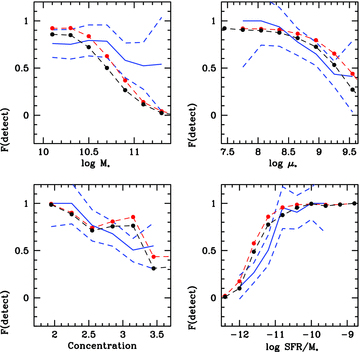
The fraction of COLD GASS galaxies with H i line detections is plotted as a function of stellar mass, stellar mass surface density, concentration and sSFR (blue curve). Poisson errors are shown as the blue dashed lines. We note that these are computed for independent bins, so the 1σ errors can be read off directly. Results for the F10 models are shown as the black (KMT atomic-to-molecular gas prescription) and red (BR pressure prescription) curves.
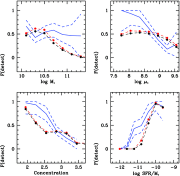
The fraction of COLD GASS galaxies with CO line detections is plotted as a function of stellar mass, stellar mass surface density, concentration and sSFR (blue curve). Poisson errors are shown as the blue dashed lines. Results for the F10 models are shown as the black (KMT atomic-to-molecular gas prescription) and red (BR pressure prescription) curves.
It is also instructive to look at the distribution of detected and non-detected galaxies in two-dimensional planes of stellar mass and galaxy structural parameters. This is illustrated in Figs 9 and 10. We plot H i/CO detected galaxies in blue and H i/CO non-detected galaxies in red in the stellar surface density versus stellar mass, concentration versus stellar mass, and concentration versus stellar surface density planes. Results from the survey are shown in the top panels and results for ‘mock catalogues’ of the same size generated from the simulations are shown in the bottom panels. In the data, there are clear thresholds in both μ* (∼3 × 10⁸ M⊙ kpc−2) and C (∼2.6) which demarcate the location of almost all galaxies without detectable gas. No such threshold is seen in stellar mass M*. This is true for both the H i and the CO non-detections.
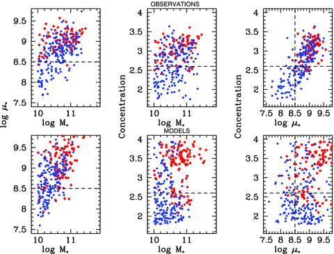
Top panels: COLD GASS galaxies are plotted in the two-dimensional planes of stellar surface density versus stellar mass, concentration versus stellar mass and concentration versus stellar surface density. Galaxies with H i line detections are plotted in blue, while those without H i line detections are plotted in red. Bottom panels: detections and non-detections from our F10 model ‘mock catalogues’ are plotted in the same three planes.
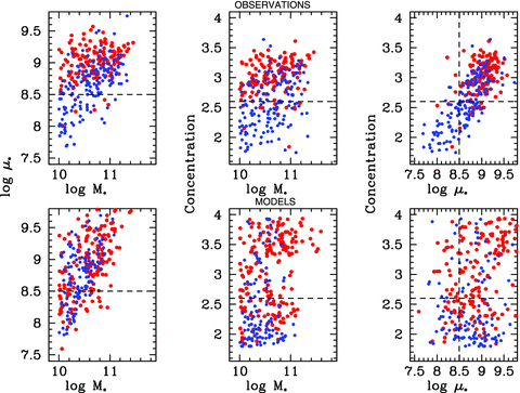
Top panels: COLD GASS galaxies are plotted in the two-dimensional planes of stellar surface density versus stellar mass, concentration versus stellar mass and concentration versus stellar surface density. Galaxies with CO line detections are plotted in blue, while those without CO line detections are plotted in red. Bottom panels: detections and non-detections from our F10 model ‘mock catalogues’ are plotted in the same three planes.
In the models, the parameters that most clearly demarcate the location of the H i non-detections are stellar mass surface density and stellar mass. It is the behaviour of the CO non-detections, however, that is most discrepant with the models. Galaxies without H2 are not confined to a specific location in structural parameter space in the same way as in the data.
We also note that the tight correlation between stellar surface density and concentration index seen in the top right-hand panels of both figures is not present in the models. In addition, the distribution of concentration indices in the models extends to much lower values than in the real data. The tight correlation between C and log μ* tells us that in the real Universe, galaxies with larger bulge-to-disc ratios have discs with higher stellar surface densities.
In the F10 models, the effects of gas inflows on the disc are not taken into account which may explain why there is no clear relation between bulge-to-disc ratio and stellar surface density. In a scenario where bulges form when gas flows inwards as a result of bar-driven inflows or other dynamical instabilities, the gas flows also increase the stellar surface mass density in the inner disc.
3.2.1 Origin of quenching thresholds in the models
We now elucidate the origin of the strong trend in the fraction of quenched galaxies as a function of stellar mass that is seen for the model galaxies. In current semi-analytic models, there are two physical processes that remove the supply of new gas to a galaxy and shut down star formation.
Radio-mode feedback. Black holes are able to grow by accreting hot gas from the surrounding halo. The growth rate is given by
 (Croton et al. 2006; Guo et al. 2011), where fhot is the ratio of hot gas mass to dark matter mass in the surrounding halo or subhalo, Vvir is the virial velocity of the halo, MBH is the black hole mass, and κ is an efficiency parameter. Some fraction of the rest-mass energy of the accreted material is assumed to be transferred to the surrounding hot gas by radio jets. The models assume an energy input rate
  , where c is the speed of light. This leads to a reduction in the cooling rate of hot gas of the form
  .
.Gas stripping. When a galaxy is accreted by a more massive dark matter halo, it becomes a ‘satellite’. In the models of De Lucia & Blaizot (2007), the hot gas surrounding the satellite is stripped instantaneously, leading to a sharp reduction in the cooling rate on to the satellite. In the more recent models of Guo et al. (2011), the dark matter and hot gas surrounding the satellite are removed more gradually both by tidal forces and by ram-pressure stripping.
The parameter κ is tuned to reproduce the high-mass end of the stellar mass function. The net effect is illustrated in Fig. 11 where we plot galaxies from our model catalogue in the two-dimensional planes of subhalo mass versus log M*, subhalo mass versus log μ*, and subhalo mass versus C. Galaxies that are predicted to be detected in CO are colour-coded in blue, while those predicted to be non-detections are colour-coded in red. Fig. 11 shows a clear transition between active and quenched galaxies at a subhalo mass of 1012 M⊙ which is a factor of ∼3 larger than the mass where dark matter haloes are predicted to transition to hosting a static halo of hot gas (Birnboim & Dekel 2003; Croton et al. 2006; Dekel & Birnboim 2006). The reason why the transition is very sharp in halo mass is because the primary dependence of the mass that is accreted by the black hole is on halo virial velocity and not on black hole mass. We note that there is an additional population of quenched galaxies in low-mass subhaloes. These are the satellite galaxies, where the subhalo has been stripped by tidal forces. As can be seen, they form a small minority of the quenched population in the stellar mass range of the galaxies in GASS.
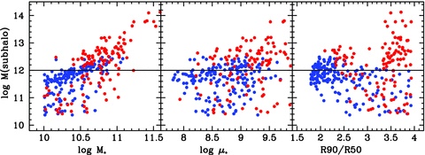
F10 model galaxies are plotted in the two-dimensional planes of subhalo mass versus stellar mass, subhalo mass versus stellar surface density and subhalo mass versus concentration. Galaxies predicted to have CO line detections are plotted in blue, while those predicted not to have CO line detections are plotted in red.
Fig. 11 clearly illustrates why quenching in the model galaxies is most strongly dependent on stellar mass and surface density, and largely independent of concentration. This is because in the model, stellar mass and surface density correlate with the virial mass of the host halo, but concentration does not. There is direct observational evidence in support of these results. Mandelbaum et al. (2006) used weak gravitational lensing to derive halo masses of galaxies as a function of stellar mass and morphology. They found stellar mass to be a good proxy for halo mass. For a given halo mass, the stellar mass was independent of concentration/morphology below M*= 1011 M⊙.
3.2.2 Origin of quenching thresholds in real galaxies
In the data, quenching thresholds are seen as a function of stellar surface density and concentration, but not as a function of stellar mass. Even for galaxies with stellar masses as high as 1011 M⊙ which are observed to reside in haloes with masses in the range 3 × 10¹²–1013 M⊙, H i and CO are generally still detected if concentrations and densities are low. This strongly suggests that processes associated with bulge formation must be responsible for shutting off the gas supply in galaxies.
We note that this hypothesis was already put forward by Kauffmann et al. (2006), based on an analysis of the scatter in the colours and spectral properties of galaxies as a function of stellar mass, stellar surface density and concentration. Kauffmann et al. (2006) made an ansatz that scatter in sSFR reflected scatter in gas content. The facts that sSFRs as well as their scatter decreased sharply above a characteristic density threshold of 3 × 10⁸ M⊙ kpc−2 and concentration index of 2.6 and that this threshold was largely independent of the stellar mass of the galaxy were taken as evidence that gas accretion was no longer occurring in bulge-dominated systems. COLD GASS and GASS have now demonstrated that the neutral gas content of galaxies is weakly dependent on stellar mass and decreases sharply at μ* > 3 × 10⁸ M⊙ kpc−2 and C > 2.6.
We have not yet ascertained why bulge-dominated galaxies no longer accrete gas and form stars efficiently. Fig. 3 shows that galaxies with μ* > 3 × 10⁸ M⊙ kpc−2 have molecular gas mass fractions that are slightly depressed relative to model predictions. Could such galaxies be transitioning to the red sequence on short time-scales as proposed by Schawinski et al. (2009)?
We note that molecular gas is generally concentrated towards the inner regions of galaxies. The SDSS fibre spectra probe the central 1–2 kpc central regions of the GASS galaxies and contain diagnostics of the recent star formation history in the bulge. In Fig. 12, we plot HδA as a function of Dn(4000) for the galaxies in the survey. Galaxies where CO was not detected are colour-coded in red, those with detections and log μ* > 8.6 are colour-coded in blue, and those with detections and log μ* < 8.6 are colour-coded in cyan. As discussed in detail in Kauffmann et al. (2003a), by combining these two stellar absorption line indices, we can diagnose if the recent star formation histories of a population of galaxies have been smooth or ‘bursty’ on average. Starbursts of duration less than 100–200 Myr displace a significant fraction of galaxies to higher values of HδA at a given value of Dn(4000). Likewise, if star formation is truncated over a time-scale of less than a few hundred million years, galaxies will also be displaced to higher than average values of HδA for around a Gyr following the truncation event (see e.g. Kauffmann et al. 2004).
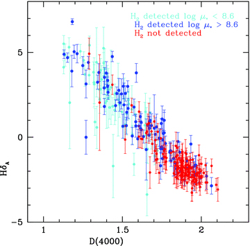
The Lick HδA index is plotted as a function of 4000 Å break strength for COLD GASS galaxies with CO line detections and log μ* > 8.6 (blue), with CO line detections and log μ* < 8.6 (cyan) and for COLD GASS galaxies with no CO line detections (red). The errors on each measurement are also indicated for each galaxy.
As can be seen, most GASS galaxies lie on the same locus in the plane of HδA versus Dn(4000). There is no evidence of any net displacement as a function of stellar surface density or as a function of H2 mass fraction, indicating that the star formation histories of most high surface density galaxies with gas have been smooth. We note, however, that galaxies with CO line detections and high stellar surface densities do span the largest range in stellar population parameters. These have Dn(4000) values as low as those of the low-density H2-rich population, and as high as those of the ‘quenched’ population. We also note that the three post-starburst galaxies that are clearly displaced to higher values of HδA, all detected in H2, have high stellar surface densities. All of them have unusually high molecular-to-atomic gas ratios, and one is clearly the end product of a recent merger (tidal features are visible in the SDSS image).
This region of parameter space is clearly quite complex, and may consist of several distinct subpopulations of galaxies on different evolutionary trajectories. If so, additional data will be required to pull these apart. In particular, studies of the distribution and kinematics of the gas may shed significant light on its origin and its eventual fate.
4 SUMMARY
We compare the semi-analytic models of galaxy formation of F10 which track the evolution of atomic and molecular gas in galaxies, with gas fraction scaling relations derived from a stellar mass-limited sample of 299 galaxies from COLD GASS. These galaxies have measurements of the CO(1–0) line from the IRAM 30-m telescope and the H i line from Arecibo, as well as measurements of stellar masses, structural parameters and SFRs derived from GALEX+SDSS photometry.
Our analysis addresses two key questions: (1) can the semi-analytic disc formation models explain the observed gas fraction scaling relations in galaxies with gas and ongoing star formation? (2) does the transition between the population of galaxies with gas and the ‘quenched’ population without gas occur in the same way in the models and in the data?
In answer to the first question, we conclude that the disc models provide a reasonable description of how condensed baryons are partitioned into stars, atomic gas and molecular gas as a function of galaxy mass and size. Trends as a function of bulge-to-disc ratio are not well reproduced. In particular, the models do not account for the fact that at fixed stellar mass, there is a tight relation between the size of a galaxy and its bulge-to-disc ratio.
In answer to the second question, we conclude that our data disagree with the current implementation of radio-mode feedback in the models. In the models, the observable parameter that best predicts whether a galaxy has been quenched is its stellar mass. Our data show that the fraction of quenched galaxies is largely independent of stellar mass, but depends strongly on galaxy bulge-to-disc ratio and stellar surface density. In other words, even low-mass galaxies with bulges have high probability of being quenched. We conclude that processes associated with bulge formation are thus likely to be responsible both for depleting the neutral gas in galaxies and for shutting off the gas supply in these systems.
Solving these problems will require substantive changes to the way gas transport and bulge and black hole formation are treated in the models, as well as to the way feedback from AGNs is implemented. We now outline our best guess as to how this might work in practice.
In the current models, newly accreted gas is assumed to have an exponential profile. If the profile is initially shallower than exponential, more atomic gas would collect in a largely inert reservoir in the outer regions of the galaxy. This gas would later be driven towards the centre of the galaxy by dynamical perturbations, where it would form molecular gas and stars in the inner region of the disc. The inflowing gas would also contribute to the growth of the bulge. A prescription of this kind may result in a better correlation between stellar surface mass density and bulge-to-disc ratio.
There is now evidence from studies of complete samples of nearby galaxies that bars are very common in disc galaxies. Barazza, Jogee & Marinova (2008) find that 70 per cent of disc-dominated galaxies host bars. Moreover, barred galaxies (in particular galaxies with strong bars) are associated with higher central molecular gas fractions and enhanced rates of central star formation (Sakamoto et al. 1999; Ellison et al. 2011; Wang et al. 2012), suggesting that bulges are forming in these systems. Finally, barred galaxies do not exhibit any excess of nearby companions, suggesting that they are not triggered by interactions (Li et al. 2009).
All of this suggests that internally driven gas transport processes are important in the formation of bulges, but resolved maps of the atomic and molecular gas distributions in complete samples of galaxies and more detailed theoretical calculation of gas inflow rates in galaxies are required in order to quantify this in more detail.
In the current models, radio-mode feedback suppresses the cooling of gas in haloes more massive than 1012 M⊙. In addition, in massive, high-density galaxies, atomic gas is transformed very efficiently into molecular gas and thence into stars. These two mechanisms appear to be sufficient to place all ‘H i-quenched’ galaxies in the high-M* and high-μ* corners of parameter space, as seen in the bottom panels of Fig. 9. The same mechanisms are not, however, sufficient to place the ‘H2-quenched’ galaxies in this same region of parameter space. Nor can they explain why galaxies deficient in both H i and H2 are almost always found in galaxies with substantial bulge components. The simplest inference is that the neutral gas in galaxies is either consumed or removed when bulges form, and that subsequent gas accretion into the atomic phase is suppressed in a significant fraction of bulge-dominated galaxies.
More detailed studies of the spatially resolved kinematics of the gas and how gas motions across galaxies correlate with the presence of accreting black holes, jets and the distribution of star formation will be needed before we are able to pinpoint the actual physical mechanisms responsible for removing/depleting the gas in these systems (see e.g. Hopkins, Quataert & Murray 2011). Quenching may occur over short time-scales during particular phases of bulge formation, so it may be necessary to survey large samples before a definitive conclusion can be reached. In addition, the mechanisms that inhibit the late accretion of gas in bulge-dominated systems remain to be clarified.
This work is based on observations carried out with the IRAM 30-m telescope. IRAM is supported by INSU/CNRS (France), MPG (Germany) and IGN (Spain). We sincerely thank the staff of the telescope for their help in conducting the COLD GASS observations and Qi Guo for helpful discussions.
Footnotes
αCO= 3.2 M⊙ (K km s−1 pc2)−1 which does not include any correction for the presence of helium.
REFERENCES
