


Abstract
We have developed further the technique of time‐dependent modelling of magnetohydrodynamic shock waves, with a view to interpreting the molecular line emission from outflow sources. The extensively observed source L1157 B1 was chosen as an exemplar of the application of this technique. The dynamical age of the shock wave model was varied in the range 500 ≤t≤ 5000 yr, with the best fit to the observed line intensities being obtained for t= 1000 yr; this is of the same order as the dynamical age derived by Gueth, Guilloteau & Bachiller from their observations of L1157 B1. The emission line spectra of H2, CO, SiO, ortho‐ and para‐H2O, ortho‐ and para‐NH3, and A‐ and E‐type CH3OH were calculated in parallel with the dynamical and chemical parameters of the model, using the ‘large velocity gradient’ (LVG) approximation to the line transfer problem. We compared the predictions of the models with the observed intensities of emission lines of H2, CO, SiO, ortho‐H2O, ortho‐NH3 and CH3OH, which include recent Herschel satellite measurements. In the case of SiO, we show (in Appendix A) that extrapolations of the collisional rate coefficients beyond the range of kinetic temperature for which they were originally calculated lead to spurious rotational line intensities and profiles. The computed emission‐line spectra of SiO, NH3 and CH3OH are shown to depend on the assumed initial composition of the grain mantles, from whence they are released, by sputtering in the shock wave, into the gas phase. The dependence of the model predictions on the adopted form of the grain‐size distribution is investigated in Appendix B; the corresponding integral line intensities are given in tabular form, for a range of C‐type shock speeds, in the online Supporting Information.
1 INTRODUCTION
It is generally accepted that the molecular line emission that is observed from outflow sources that are associated with low‐mass star formation is produced predominantly in shock waves, which are generated by the interaction between the outflow and the ambient medium. In the presence of a magnetic field, these (C‐type) shock waves have precursors in which the charged and neutral fluids flow at different speeds and their kinetic temperatures differ. The inertia of (charged) dust grains affects the ion‐neutral drift speed and hence the thermal and chemical structure of the shock wave. In order to predict the intensities of the molecular lines that are emitted by such regions, a magnetohydrodynamic (MHD) model must treat, in a self‐consistent manner, not only the dynamical and the chemical processes but also the transfer of the molecular line radiation through the medium.
Recent applications of MHD shock wave models to the study of outflow sources are to be found in Gusdorf et al. (2008a,b), Flower, Pineau des Forêts & Rabli (2010) and Viti et al. (2011). In all of these studies, the treatment of the shock wave dynamics derives from the work of Flower & Pineau des Forêts (2003), who considered the electrical charging of the grains and their influence on the dynamical and chemical profiles of the shock wave. As these objects are young, with ages of the order of 103 yr, the shock wave is unlikely to have reached steady state. As was first shown by Chièze, Pineau des Forêts & Flower (1998), in the presence of a magnetic field, transverse to the direction of flow, a shock wave evolves from J‐ to C‐type on a time‐scale of typically a few thousand years and possesses both C‐ and J‐type characteristics at intermediate times. Accordingly, it is more realistic to model the emission from outflow sources by means of such CJ‐type shock waves, comprising a J‐ as well as a C‐type component, which are characteristic of flows that have yet to attain steady state. Such models were presented and discussed by Gusdorf et al. (2008b), who considered the rovibrational spectrum of H2 and the rotational transitions of CO and SiO. However, this study predates the Herschel measurements, to which reference will be made below; these more recent observational data extend to additional molecular species and thereby provide valuable supplementary constraints on the models.
L1157 is perhaps the most extensively observed molecular outflow that is associated with the formation of a low‐mass star. Recently, it was a priority target of the key programmes CHESS and WISH, following the commissioning of the Herschel satellite. These initial observations (Ceccarelli et al. 2010; Codella et al. 2010; Lefloch et al. 2010; Nisini et al. 2010a) showed that the blue (B1) component has a rich submillimetre and far‐infrared emission‐line spectrum, containing transitions of CO, CH3OH, H2O, NH3 and other molecular species. Rovibrational transitions of H2 from this same source had been observed previously, from the ground (Caratti o Garatti et al. 2006), and pure rotational transitions of H2 have been observed by means of the Infrared Space Observatory (ISO) satellite (Cabrit et al. 1999) and the Spitzer Space Telescope (Nisini et al. 2010b). In addition, there have been ISO observations of high‐J rotational transitions of CO (Giannini, Nisini & Lorenzetti 2001) and ground‐based observations of rotational transitions of SiO (Nisini et al. 2007). Thus, L1157 B1 has become a prime observational target when studying molecular outflow sources, and further Herschel observations, involving additional transitions and species, may be expected.
The high energies that are required to excite some of the observed transitions and the morphology of L1157 B1 are factors which point to the excitation of the molecular line emission being induced by a shock wave, generated by the impact of the outflowing material on the ambient molecular cloud. Given the dynamical age of the blue lobe of the L1157 outflow, which has been estimated to be only 2000–3000 yr (Gueth, Guilloteau & Bachiller 1998), the shock wave is unlikely to have reached steady state. The C‐ and CJ‐type shock wave models that we have used to simulate the spectrum of L1157 B1 incorporate a number of significant improvements on the work of Gusdorf et al. (2008b) and the more recent study of methanol by Flower et al. (2010). The emission‐line spectra of CO, SiO, ortho‐ and para‐H2O, ortho‐ and para‐NH3, and A‐ and E‐type CH3OH are all computed in a completely self‐consistent manner within the shock wave model, applying a large‐velocity‐gradient (LVG) approximation to the line transfer problem. This approach has a number of advantages over the method adopted by Gusdorf et al. (2008b), in which the profiles of the dynamical and chemical variables, generated by the shock code, were used as input to separate and independent LVG computations of the molecular line emission. One significant advantage is that the total rate of molecular cooling can be determined point by point in the model and incorporated in the simultaneous calculation of the thermal profile of the shock wave.
In Section 2, we present the pertinent features of the model and specify the sources of the molecular data that have been used. In Section 3, we compare the predictions of CJ‐type models with the available ground‐based and satellite observations of L1157 B1. Our concluding remarks are made in Section 4.
2 MODEL
We note the expression for the velocity gradient of the neutral fluid, dvn/dz, is a function of, amongst other quantities, the local rate of cooling of the gas by molecular line radiation. In the context of the LVG approximation to the line transfer, the optical depths in the lines, and hence the rate of cooling by escaping photons, depend on the velocity gradient of the neutral fluid. This interdependence is treated by means of an iterative method, which ensures convergence of the velocity gradient to within a specified tolerance, taken in practice to be 0.0001 per cent.
We have considered a range of shock types and parameters (initial conditions), taking the earlier studies of G08a,b as a guide. Reference will be made to some of these results below, but the discussion will be concerned mainly with the CJ‐type shock wave of speed vs= 20 km s−1, propagating into molecular gas of density nH≈ 2n(H2) +n(H) = 104 cm−3, with an initial transverse magnetic field strength B= 100 μG. The dynamical age, which is determined in the model by the flow time of the ionized fluid, ti, to the J‐discontinuity (G08b, appendix C), was varied in the range 500 ≤t≤ 5000 yr. Following G08b, we terminated the integration when ti reached twice the dynamical age, where the medium is approaching its post‐shock equilibrium state. For comparison purposes, we computed also the steady‐state solution, i.e. we ran the corresponding C‐type model.
2.1 Molecular data
The sources of molecular data (level energies, radiative transition probabilities and collisional rate coefficients) for CO (Flower & Gusdorf 2009),1 CH3OH (Flower et al. 2010), H2O (Flower & Pineau des Forêts 2010) and SiO (G08a) have been given previously. Many of these data have been accessed through the Leiden Observatory database, LAMDA (Schöier et al. 2005). In the cases of ortho‐ and para‐NH3, rate coefficients for excitation only by He (Machin & Roueff 2005) and by para‐H2 (Danby et al. 1988) in its rotational ground state, J= 0, are available; we adopted the para‐H2 rate coefficients for collisions with ortho‐H2 and with H.
We note that some of the sets of rate coefficients for collisional transfer that are available in the LAMDA database, notably for SiO, have been extrapolated, both to higher kinetic temperatures and to more highly excited rotational levels than were included in the original collision calculations. The potential hazards associated with such extrapolations, particularly as functions of temperature, are illustrated by the example of SiO, considered in Appendix A.
2.2 Chemistry
The chemistry of the medium, including the initial composition of the gas and the solid phases, is significant in determining the intensities of the lines of all the molecular species that we have considered, with the possible exception of CO. Nitrogen‐containing species, specifically NH3, CN, HCN, HNC and N2H+, are particularly important for the diagnostics of pre‐stellar cores, providing information on the evolution of the object during its approximately isothermal, low‐temperature (T≈ 10 K), pre‐collapse phase (see, for example, Belloche & André 2004; Flower, Pineau des Forêts & Walmsley 2006). Some of the current estimates of the rates of reactions leading to the formation or destruction of nitrogen‐containing species at such low temperatures may be unreliable. However, the higher kinetic temperatures relevant to shock waves overlap the temperature range of the majority of laboratory measurements, and hence the rates of reaction under shock conditions should be more secure.
In cold gas, the formation of nitrogen‐containing species, such as NH3, is believed to be initiated by the reaction of N2 with He+, which yields N+. Sequences of hydrogen‐abstraction reactions with H2 then lead to NH , which recombines dissociatively to form NH3. The preliminary formation of N2 occurs in the neutral–neutral reactions N(OH, H)NO and NO(N, O)N2, or N(CH, H)CN and CN(N, C)N2 (cf. Hily‐Blant et al. 2010), whose rates of reaction at T≈ 10 K are sensitive to the possible existence of even small reaction barriers. The formation of NH3 in shock‐heated gas, on the other hand, occurs mainly in the reactions N(H2, H)NH, NH(H2, H)NH2 and NH2(H2, H)NH3. Although these reactions are endothermic and/or have barriers (see Table 1), the kinetic temperatures that are attained in shock waves with speeds vs≳ 15 km s−1 are sufficient to ensure that these reactions dominate the production of NH3. For shock speeds vs≳ 30 km s−1, the reverse reactions with H (produced by the collisional dissociation of H2) become significant in reducing the fractional abundance of NH3 in the gas phase.
Rate coefficients of the reactions leading to the formation and destruction of NH3 in hot, shocked gas. The original sources of the data from the NIST database (http://spec.jpl.nasa.gov) are listed. The rate coefficient at kinetic temperature T is expressed as k=γ(T/300)αexp (−β/T).
| Reaction | γ (cm3 s−1) | α | β (K) | Reference |
| N(H2, H)NH | 6.85 × 10⁻¹⁰ | 0.00 | 12 990 | Pascual et al. (2002) |
| NH(H2, H)NH2 | 3.50 × 10⁻¹¹ | 0.00 | 7 760 | Fontijn et al. (2006) |
| NH2(H2, H)NH3 | 6.75 × 10⁻¹⁴ | 2.60 | 3 007 | Friedrichs & Wagner (2000) |
| NH3(H, H2)NH2 | 6.54 × 10⁻¹³ | 2.76 | 5 170 | Corchado & Espinosa‐Garcia (1997) |
The other source of gas‐phase ammonia in shock waves is NH3 that is initially in the form of ice in the grain mantles. When the shock speed vs≳ 15 km s−1, the mantles are eroded, owing to collisions of the predominantly negatively charged grains with the abundant neutral species H2, H and He, at the ion‐neutral drift speed. Observations of W33 A by Gibb et al. (2000) lead to a fractional abundance of ammonia ice  in the grain mantles, which is orders of magnitude greater than the initial abundance of ammonia in the gas phase. Of course, the relevance of this observation of W33 A to conditions in L1157 B1 is open to question. As we shall see in Section 3, the intensity of the 572 GHz line of ortho‐NH3– observed in L1157 B1 by means of Herschel/HIFI (Codella et al. 2010) – suggests that the initial abundance of NH3 ice is much less than the observations of W33 A would imply; a similar conclusion is reached in the case of CH3OH.
2.3 Grain size
An issue that needs to be addressed when modelling interstellar shock waves is the size distribution of the grains in the medium. The grains become predominantly negatively charged in the shock wave (Flower & Pineau des Forêts 2003; Guillet, Pineau des Forêts & Jones 2007), and their inertia affects significantly the thermal profile of the neutral gas, owing to the coupling between the charged and neutral fluids. The strength of this coupling depends of the gas–grain collision rate and hence on the mean value of  , where ng is the grain number density and ag is the grain radius. For a given total grain mass, this product is inversely proportional to ag, and so charged grains that are larger, on average, couple less effectively to the neutral gas. As a consequence, the neutral temperature profile, as a function of distance through the shock wave, becomes wider and flatter.
The grain‐size distribution of Mathis, Rumpl & Nordsieck (1977) has been used extensively in studies of the interstellar medium, and this distribution has been adopted both in the present work and by G08a,b. However, it should be recalled that the observations, from which the distribution of Mathis et al. (1977) was deduced, related to the diffuse interstellar medium, rather than denser, molecular gas. There is some indirect evidence, from studies of prestellar cores (see Walmsley, Flower & Pineau des Forêts 2004), that grains and large molecules, such as the polycyclic aromatic hydrocarbon (PAH), may have coagulated. Accordingly, we have considered, in addition to the size distribution of Mathis et al. (1977), grains with a larger mean size of up to 0.5 μm; see Appendix B.
As mentioned in Section 2.2, the grains in the cold, pre‐shock gas are assumed to have ice mantles of a specified composition. The mantles are eroded in the shock wave, principally through sputtering by the most abundant neutral species. Subsequently, as the gas cools towards its post‐shock temperature, partial freeze‐out of the gas‐phase species on to the grains occurs. Owing to the removal or the acquisition of a mantle, the radius of the grains, and hence the strength of their coupling to the gas, varies. The radius of the grains was calculated following the approach of Le Bourlot et al. (1995, appendix A), adopting a numerical value of 3 g cm−3 for the density of the grain material and 3.4 × 10⁻⁸ cm for both the mean distance between binding sites and the thickness of a layer of the mantle.
3 RESULTS AND DISCUSSION
G08b discussed in some detail the predictions of CJ‐type models for ranges of the shock parameters, notably the shock speed, vs, the pre‐shock gas density, nH, the pre‐shock magnetic field strength, B, and the dynamical age of the shock wave, t. Our intention here is to extend their application of the shock code to simulating the spectrum of L1157 B1, making use of the recent CHESS and WISH data. In the light of the results from a preliminary analysis, comparison will be made with the CJ‐type model in which vs= 20 km s−1, nH= 104 cm−3 and B= 100 μG. The initial fractional abundances that were adopted for the principal chemical species, in both the gas and solid (ice) phases, are listed in Table 2 and considered below.
Initial fractional abundances, relative to nH≈ 2n(H2) +n(H), of the principal chemical species of the model. Constituents of the ice mantles of the grains are identified by an asterisk. PAH is the representative polycyclic aromatic hydrocarbon molecule, and G denotes the grains, which are assumed to have the grain‐size distribution of Mathis et al. (1977), for grain radii 0.3 ≥ag≥ 0.01 μm. Numbers in parentheses are powers of 10.
| Species | Fractional abundance |
| H2 | 5.00 (−01) |
| He | 1.00 (−01) |
| O | 6.25 (−06) |
| O2 | 4.18 (−06) |
| H2O | 1.88 (−07) |
| CO | 8.20 (−05) |
| N | 2.00 (−06) |
| N2 | 3.08 (−05) |
| S | 1.39 (−05) |
| PAH | 9.63 (−07) |
| G | 4.30 (−11) |
| H2O* | 1.03 (−04) |
O | 1.35 (−05) |
| CO* | 8.26 (−06) |
CO | 1.34 (−05) |
CH | 1.55 (−06) |
NH | 1.55 (−06) |
N | 6.97 (−06) |
| CH3OH* | 3.10 (−06) |
| H2CO* | 6.19 (−06) |
H2CO | 7.23 (−06) |
| OCS* | 2.07 (−07) |
| H2S* | 3.72 (−06) |
| SiO* | 2.67 (−06) |
| S+ | 1.19 (−08) |
| PAH+ | 1.28 (−09) |
| G+ | 1.23 (−12) |
| PAH− | 3.61 (−08) |
| G− | 2.02 (−12) |
| Species | Fractional abundance |
| H2 | 5.00 (−01) |
| He | 1.00 (−01) |
| O | 6.25 (−06) |
| O2 | 4.18 (−06) |
| H2O | 1.88 (−07) |
| CO | 8.20 (−05) |
| N | 2.00 (−06) |
| N2 | 3.08 (−05) |
| S | 1.39 (−05) |
| PAH | 9.63 (−07) |
| G | 4.30 (−11) |
| H2O* | 1.03 (−04) |
| O | 1.35 (−05) |
| CO* | 8.26 (−06) |
| CO | 1.34 (−05) |
| CH | 1.55 (−06) |
| NH | 1.55 (−06) |
| N | 6.97 (−06) |
| CH3OH* | 3.10 (−06) |
| H2CO* | 6.19 (−06) |
| H2CO | 7.23 (−06) |
| OCS* | 2.07 (−07) |
| H2S* | 3.72 (−06) |
| SiO* | 2.67 (−06) |
| S+ | 1.19 (−08) |
| PAH+ | 1.28 (−09) |
| G+ | 1.23 (−12) |
| PAH− | 3.61 (−08) |
| G− | 2.02 (−12) |
Initial fractional abundances, relative to nH≈ 2n(H2) +n(H), of the principal chemical species of the model. Constituents of the ice mantles of the grains are identified by an asterisk. PAH is the representative polycyclic aromatic hydrocarbon molecule, and G denotes the grains, which are assumed to have the grain‐size distribution of Mathis et al. (1977), for grain radii 0.3 ≥ag≥ 0.01 μm. Numbers in parentheses are powers of 10.
| Species | Fractional abundance |
| H2 | 5.00 (−01) |
| He | 1.00 (−01) |
| O | 6.25 (−06) |
| O2 | 4.18 (−06) |
| H2O | 1.88 (−07) |
| CO | 8.20 (−05) |
| N | 2.00 (−06) |
| N2 | 3.08 (−05) |
| S | 1.39 (−05) |
| PAH | 9.63 (−07) |
| G | 4.30 (−11) |
| H2O* | 1.03 (−04) |
| O | 1.35 (−05) |
| CO* | 8.26 (−06) |
| CO | 1.34 (−05) |
| CH | 1.55 (−06) |
| NH | 1.55 (−06) |
| N | 6.97 (−06) |
| CH3OH* | 3.10 (−06) |
| H2CO* | 6.19 (−06) |
| H2CO | 7.23 (−06) |
| OCS* | 2.07 (−07) |
| H2S* | 3.72 (−06) |
| SiO* | 2.67 (−06) |
| S+ | 1.19 (−08) |
| PAH+ | 1.28 (−09) |
| G+ | 1.23 (−12) |
| PAH− | 3.61 (−08) |
| G− | 2.02 (−12) |
It may be seen in Fig. 1 that, as the age of the shock wave increases in the range 500 ≤t≤ 5000 yr, the J‐discontinuity weakens until it is no longer present in the limit of steady state, when the shock becomes C‐type. Thus, the shock wave displays predominantly J‐type characteristics in its youth and C‐type characteristics as it approaches its final equilibrium state. In dynamically young objects, such as molecular outflows, shock waves may be expected to have mixed, J‐ and C‐type, characteristics.
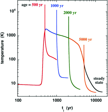
Thermal profile of the neutral fluid, as computed for a CJ‐type shock wave of speed vs= 20 km s−1, propagating into molecular gas of density nH≈ 2n(H2) +n(H) = 104 cm−3, with an initial transverse magnetic field strength B= 100 μG. The independent variable in this figure is the flow time of the ionized fluid, ti. The dynamical age was varied in the range 500 ≤t≤ 5000 yr. The corresponding C‐type model (i.e. the steady‐state solution, attained by t≈ 10 000 yr) is shown for comparison purposes. As the shock wave ages, the J‐discontinuity moves to the right, becoming progressively weaker as equilibrium is approached.
3.1 CO emission
High‐J transitions of CO in a sample of 17 Class 0 outflow sources, including L1157, were observed with the ISO Long‐Wavelength Spectrometer (LWS), and the line fluxes were derived by Giannini et al. (2001); the corresponding integrated line intensities, TdV, are plotted in Fig. 2. Also shown in this figure are the intensity of the J= 5 → 4 transition, observed with the Herschel/HIFI instrument (Codella et al. 2010), and the intensities of the J= 3 → 2 and J= 6 → 5 lines, reported by Lefloch et al. (2010), which were derived from Caltech Submillimeter Observatory (CSO) observations and smoothed to the 39 arcsec diameter of the HIFI band 1b beam. The line intensities predicted by the CJ‐type model are also plotted.
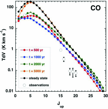
Observed and computed intensities of the rotational transitions Jup→Jup− 1 of CO; see the text, Section 3.1. Error bars that are not apparent are smaller than the size of the symbol used to plot the corresponding line intensities. Error bars for the J= 3 → 2 and J= 6 → 5 lines, derived from CSO observations by Lefloch et al. (2010), were not quoted by these authors.
3.2 SiO emission
The intensities of the lines emitted by the rotational levels J= 2, 3, 5, 6, 8 and 10 of SiO were observed from L1157 B1 by Nisini et al. (2007). The 10 → 9 and 8 → 7 transitions were observed with the James Clerk Maxwell Telescope, and the other lines by means of the IRAM 30‐m telescope. At the frequency of the J= 8 → 7 transition, the half‐power beam width (HPBW = ) appears to be approximately half of the diameter of the emitting region (Nisini et al. 2007, fig. 3), in which case the filling factor would be approximately unity. On the other hand, the HPBW increases towards lower frequencies, reaching 27.6 arcsec for the J= 2 → 1 transition. Furthermore, interferometric observations of the J= 5 → 4 and J= 2 → 1 transitions (Gueth et al. 1998) show that the SiO‐emitting region is only around
  in diameter. When the size of the beam is comparable to the angular size of the emitting region, the filling factor ≈0.5. Increasing the observed intensities of the low‐J transitions by the inverse of the filling factor would result in better agreement with the predictions of the youngest CJ‐type models (cf. Fig. 3).
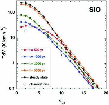
Observed and computed intensities of the rotational transitions Jup→Jup− 1 of SiO; see the text, Section 3.2. Error bars that are not apparent are smaller than the size of the symbol used to plot the corresponding line intensities.
In Fig. 3 are plotted the observed and predicted (by the CJ‐type models) intensities of the SiO transitions. The model assumes that 8 per cent of the elemental silicon is initially in the form of SiO in the grain mantles. The mantles are eroded rapidly in the shock wave, and the resulting gas‐phase SiO is excited collisionally, principally by H2. We used the rate coefficients calculated by Dayou & Balança (2006), for excitation by He, scaled (by a factor of 1.38) to the reduced mass of H2. For the reasons given in Appendix A, we used the rate coefficients in the LAMDA data base only for the ranges of rotational quantum number, J, and kinetic temperature, T, for which they had been calculated by Dayou & Balança (2006). The dangers inherent in extrapolating their data to higher temperature are illustrated in Appendix A.
The comparisons in Fig. 3 are indicative, once again, of a low dynamical age, with t= 1000 yr yielding the best overall fit. The calculated 2 → 1 line intensity exceeds the observed value, though by no more than a factor of about 2. Furthermore, the computed value of the intensity this low‐J transition depends on the adopted cut‐off (in the post‐shock gas) of the integration with respect to distance through the shock wave: earlier termination of the integration results in a lower 2 → 1 line intensity.
3.3 H2 emission
The usual way of comparing with the observed intensities of the rovibrational transitions of H2 is via the so‐called excitation diagram. Because the H2 rovibrational spectrum is quadrupolar, the radiative transition probabilities are small and there is a tendency towards thermalization of the rotational level populations, within a given vibrational manifold. In addition, the lines are optically thin. Thus, it can be meaningful to plot log (NvJ/gJ) versus EvJ (the ‘excitation diagram’), where NvJ cm−2 is the column density of the rovibrational level vJ, deduced from the line intensities, gJ= (2J+ 1)(2I+ 1), where I= 1 for ortho‐H2 and I= 0 for para‐H2 is the total nuclear spin quantum number, and EvJ is the excitation energy of the level vJ, in K, relative to the v= 0 =J ground state.
It may be seen from the excitation diagram, plotted in Fig. 4, that the CJ‐type model with t= 1000 yr best reproduces the observed column densities, with the exception of levels in the v= 1 manifold, whose column densities are underestimated by all of the models. Fig. 4 includes the column densities deduced from the ISO observations of rotational transitions within the v= 0 vibrational ground state (Cabrit et al. 1999). The more recent Spitzer observations of the intensities of v= 0 J→J− 2 transitions emitted by the B1 source (Nisini et al. 2010b) yield column densities that are in good agreement with the earlier measurements for low‐J levels but are smaller, by factors of up to approximately 4, for high J. However, the interpretation of the excitation diagram is not significantly affected by adopting the more recent measurements. In this calculation, it was assumed that the process of reformation of H2, on grains, results in the rovibrational levels being repopulated in proportion to gJexp (−EvJ/17 249), the statistical (Boltzmann) factor at a temperature of 17 249 K, which is 1/3 of the H2 dissociation energy. In practice, the way in which the reformation process populates the levels of H2 is still uncertain. The selective population of the v= 1 levels would enhance their computed column densities, but we are not aware of any independent evidence that supports such a hypothesis.
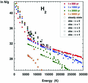
Observed and computed H2 excitation diagram. N is the column density (cm−2) of the emitting rovibrational level, (v, J), and g= (2J+ 1)(2I+ 1) is its degeneracy (the nuclear spin quantum number I= 1 for ortho‐H2, and I= 0 for para‐H2). Observed values of ln N/g are plotted against the excitation energy of the emitting level, together with the values computed at the four dynamical ages indicated, and in the limit of steady state. See the text, Section 3.3.
As noted by G08b, the smaller the dynamical age of the shock wave, the greater is the maximum kinetic temperature that is attained and the higher are the populations of the vibrationally excited levels. Consequently, models with larger dynamical ages tend to underestimate the column densities of levels with v > 0, as may be seen in Fig. 4. It should be recalled that the shock wave in L1157 is more likely to be bow type than plane parallel, as is assumed by the model. To the varying angle of attack along the bow profile, there corresponds a range of effective shock speeds, with the highest speed being attained at the apex of the bow. It is remarkable that a single, plane‐parallel CJ‐type model is able to reproduce the observed H2 column densities and is seen to be the case in Fig. 4.
3.4 CH3OH emission
Several transitions of both A‐ and E‐type methanol have been observed in emission from L1157 B1 by Codella et al. (2010); the energies of the emitting levels extend up to approximately 210 K. Adopting the initial fractional abundance of methanol ice, n(CH3OH*)/nH= 1.9 × 10⁻⁵, from the observations of W33 A by Gibb et al. (2000) leads to computed methanol line intensities (for the reference CJ‐type model) that exceed systematically the observed values, by a factor of approximately 6. Of course, the abundance of methanol ice in L1157 B1 may differ from that observed in W33 A. If the initial value is reduced, by a factor of 6, to n(CH3OH*)/nH= 0.3 × 10⁻⁵, the methanol line intensities predicted by the model with dynamical age t= 1000 yr are found to be in good overall agreement with those observed, as may be seen in Fig. 5. Once again, these comparisons lead to the exclusion of large dynamical ages.
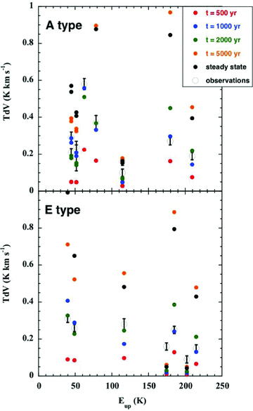
Observed and computed intensities, TdV, of the rotational transitions of A‐ and E‐type CH3OH, plotted against the excitation energy of the emitting level, Eup, expressed relative to the energy of the J= 0 =K ground state of A‐type. See the text, Section 3.4.
Bachiller et al. (1995) observed a number of lines of CH3OH in L1157 with the IRAM 30‐m telescope. The only unblended line is A+ 30– 20 at 145.1 GHz, whose integral intensity, at the position of the B1 source and in a beam of HPBW = 17 arcsec, was 44.5 ± 0.3 K km s−1. In the sense of increasing dynamical age, our CJ‐type models predict 2.5 K km s−1 (t= 500 yr), 13.4 K km s−1 (t= 1000 yr), 21.6 K km s−1 (t= 2000 yr) and 63.2 K km s−1 (t= 5000 yr); in steady state, the predicted integral intensity is 84.7 K km s−1. However, we note that the excitation energy of the upper level of this transition is only approximately 14 K, and it follows that it may be excited in the compressed post‐shock gas, whose contribution to the integral line intensity has been excluded from the model predictions.
3.5 Ortho‐H2O and ortho‐NH3 emission
Codella et al. (2010) observed the transitions between the first excited and the ground states of ortho‐H2O and ortho‐NH3, at 557 and 572 GHz, respectively. The observed intensity of the ortho‐H2O line was 11.7 ± 0.1 K km s−1, and that of the ortho‐NH3 line was 0.89 ± 0.03 K km s−1.
In Fig. 6, we plot, as a function of the excitation energy of the emitting level, the computed intensities of the lines of ortho‐ and para‐H2O2 which fall in the Herschel/HIFI bands, including the 557 GHz line of ortho‐H2O, whose observed intensity is also plotted. In this case, the best agreement is obtained for t= 500 yr, although the line intensity predicted by the t= 1000 yr model is within a factor 2 of that observed. We note that, in the study of Flower et al. (2010), there was an error in the determination of the velocity gradient of the neutral fluid in the region downstream of the J‐discontinuity in the CJ‐type model. As a consequence, the optical depth in the 557 GHz line was underestimated and the intensity of this transition was overestimated. The corresponding plots for ortho‐ and para‐NH33 are shown in Fig. 7.
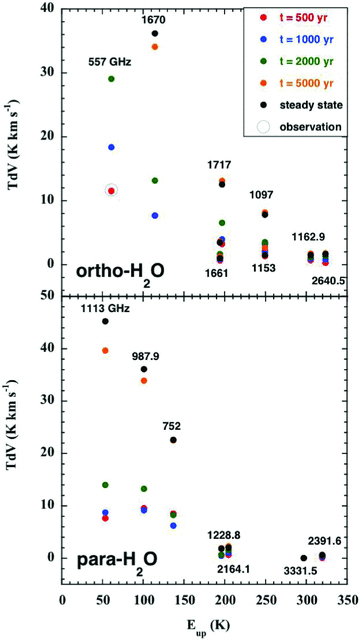
Computed intensities of the rotational transitions of ortho‐ and para‐H2O, plotted against the excitation energy of the emitting level, expressed relative to the energy of the J= 0 =K ground state of para; the intensity of the 557 GHz line of ortho‐H2O, observed by Codella et al. (2010), is also plotted. See the text, Section 3.5. The error bar associated with the observed line intensity is not visible on the scale of this figure.
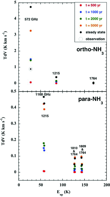
Computed intensities of the rotational transitions of ortho‐ and para‐NH3, plotted against the excitation energy of the emitting level, expressed relative to the energy of the J= 0 =K ground state of ortho; the intensity of the 572 GHz line of ortho‐NH3, observed by Codella et al. (2010), is also plotted. See the text, Section 3.5.
The initial abundance of water ice was adopted from Flower & Pineau des Forêts (2003) and derives from the observations of Gibb et al. (2000); the initial gas‐phase abundance of water was evaluated in chemical equilibrium. However, this same approach leads, in the case of NH3, to the overestimation the intensity of the 572 GHz line, by a factor of approximately 6 for the t= 1000 yr model. That the discrepancy for ortho‐NH3 is of the same magnitude and in the same sense as for the methanol lines may not be coincidental. As noted in Section 2.2, the initial abundance of ammonia in the grain mantles is much larger than that in the gas phase. The formation of NH3 in the gas phase can proceed rapidly in shock‐heated gas, via the sequence of hydrogen‐abstraction reactions with H2, considered in Section 2.2. However, this sequence is initiated by the reaction of H2 with atomic N, and so the production of ammonia is inhibited if most of the gas‐phase nitrogen is in the form of N2, as was suggested by Hily‐Blant et al. (2010), on the basis of their study of prestellar cores. In order to test these hypotheses, we ran a model in which the initial abundance of ammonia ice was reduced by an order of magnitude to  , with the fraction of elemental nitrogen in the solid phase being maintained constant by its reallocation to N2 ice. Similarly, in the gas phase, the initial fractional abundance of atomic N was reduced to n(N)/nH= 2.0 × 10⁻⁶, whilst that of N2 was increased correspondingly to n(N2)/nH= 3.1 × 10⁻⁵. In this case, the intensity of the 572 GHz line of ortho‐NH3, predicted by the t= 1000 yr model, fell to 1.6 K km s−1, which is within a factor of 2 of the observed value. As may be seen from Fig. 7, the model with a dynamical age of 2000 yr provides an equally acceptable fit, whereas the 500 and 5000 yr models, respectively, underestimate and overestimate the line intensity.
Tafalla & Bachiller (1995) observed the B1 source in the (J, K) = (3, 3) and (1, 1) inversion transitions of ortho‐ and para‐NH3, respectively, using the Very Large Array, and their discussion suggests that the integral line intensities, deduced from the profiles plotted in fig. 3 of their paper, may be compared sensibly with the predictions of the models; the (observed) integral intensity of the (3, 3) transition is approximately 13 K km s−1, and that of the (1, 1) transition is approximately 3 K km s−1. The intensities predicted by the CJ‐type model with an age t= 500 yr are 1.1 and 0.3 K km s−1; at t= 1000 yr, the corresponding intensities are 33 and 14 K km s−1. Thus, these ground‐based observations of NH3 lines are also consistent with a dynamical age 500 < t < 1000 yr.
As may be seen in Fig. 1, the maximum temperature of the neutral fluid attained in the magnetic precursor of our CJ‐type model, in which vs= 20 km s−1 and the pre‐shock density nH= 104 cm−3, is approximately 2000 K. This maximum temperature is to be compared with the value of 2200 K obtained by Viti et al. (2011; models 7 and 14) for a (parametric) C‐type shock wave model in which vs= 40 km s−1 and nH= 2 × 104 cm−3. We remark that our corresponding C‐type model predicts a higher maximum temperature of approximately 4000 K; the tendency for the parametric model to underestimate the maximum temperature in the shock wave is noted by Viti et al. (2011). The significance of this discrepancy for the relative abundance and the line profiles of NH3 and H2O is discussed further in Appendix B.
Viti et al. (2011) considered the recent Herschel observations of ammonia line profiles from the B1 source. Their conclusion – that a C‐type shock wave with a maximum temperature of 4000 K can reproduce these observations – is reached without consideration of the additional molecular line observations of this source discussed here. It was shown conclusively by G08b, and confirmed by the present study, that steady‐state (C‐type) shock waves are unable to reproduce the empirical H2 excitation diagram of the B1 source. We find that models reflecting the CJ‐type structure of the shock wave, at dynamical ages much smaller than the time that is required to reach steady state, are indispensable to interpreting available observations of the plethora of molecular lines emitted by this source, and even these models undoubtedly oversimplify the true structure of L1157 B1.
4 CONCLUDING REMARKS
We have modelled the molecular line emission from the L1157 B1 outflow source. We find that the observed intensities of emission lines of CO, SiO and ortho‐H2O can be reproduced satisfactorily by a CJ‐type shock wave model, with a speed vs= 20 km s−1, pre‐shock gas density nH= 104 cm−3 and initial magnetic field strength B= 100 μG. The dynamical age of the shock wave model was varied in the range 500 ≤t≤ 5000 yr; the best fit to the observed line intensities was obtained for t= 1000 yr, which is of the same order as the dynamical age that has been derived from observations of the B1 source (Gueth et al. 1998). In connection with the rotational lines of SiO and their profiles, we demonstrate that the extrapolation of collisional rate coefficients over a wide range of kinetic temperatures can lead to spurious results, and we caution against the use of such extrapolated data.
The model reproduces satisfactorily the intensity of the 572 GHz transition of ortho‐NH3 and the intensities of the CH3OH lines when the initial abundances of ammonia and methanol ice, in the grain mantles, are reduced by factors of approximately 10 and 6, respectively, relative to the measurements by Gibb et al. (2000) from their observations of W33 A. The mantles undergo sputtering in the shock wave, releasing the ice into the gas phase. In the case of ammonia, there is an additional requirement that a large fraction of the elemental nitrogen should be in the form of N2, rather than atomic N, in the pre‐shock gas, as suggested by a recent study of prestellar cores (Hily‐Blant et al. 2010).
The model underestimates the column densities of the v= 1 levels of H2 but otherwise reproduces faithfully the empirical excitation diagram. The discrepancy in the case of the v= 1 manifold might be attributable, at least in part, to preferential population of the v= 1 states during the process of reformation of H2, on grain surfaces, in the wake of the shock wave; but empirical confirmation of the existence this selective population mechanism is required.
Given the likelihood that the shock wave in L1157 B1 is a bow shock, rather than the plane‐parallel structure that is modelled, we consider that the overall level of agreement between the observations and the predictions of the non‐stationary, CJ‐type shock wave model is encouraging.
Footnotes
The results of the recent calculations by Yang et al. (2010) of the rate coefficients for excitation by ortho‐ and para‐H2 were used in the present study, when computing the CO level populations. The results of Yang et al. extend to larger values of the rotational quantum number (J≤ 40) and to higher kinetic temperatures (T≤ 3000 K) than the earlier calculations by Flower (2001), which were used by Flower & Gusdorf (2009). We found that the computed line intensities were essentially identical for transitions from rotational levels that are common to the data sets of Flower (2001) and of Yang et al. (2010).
The ortho:para ratio was assumed to take its statistical value of 3.
The ortho:para NH3 ratio was assumed to take its statistical value of 1.
The integration was terminated at the point at which the temperature of the neutral fluid had fallen to 15 K.
REFERENCES
Appendices
APPENDIX A: SiO LINE PROFILES
The calculations of Dayou & Balança (2006), of the rate coefficients for the excitation of SiO by He, extended up to a kinetic temperature T= 300 K and to the rotational state J= 26, whose excitation energy, relative to the J= 0 ground state, is approximately 1700 K. In shock waves, the kinetic temperature can attain values of the order of 103–104 K, implying a need for rate coefficients at higher temperatures and for larger values of J. It is unsurprising, therefore, that methods for extrapolating the rate coefficients, in both T and J, have been developed: see Schöier et al. (2005).
In the case of SiO–He collisions, the results of Dayou & Balança (2006) display a propensity for transitions in which the rotational quantum number of SiO changes by ΔJ= 1. Given the large dipole moment of SiO (of approximately 3 debye), such a propensity was to be anticipated. As a consequence, one expects that the high‐J levels of SiO to be populated predominantly through a step‐by‐step process, involving collisional excitation …J− 1 →J→J+ 1… .
The situation is very different for transitions involving large values of ΔJ; see Fig. A1. The computed values of the rate coefficients for such (de‐excitation) transitions remain much smaller than for transitions involving small values of ΔJ, particularly ΔJ= 1, up to the limit of the calculations by Dayou & Balança (2006), but tend to increase with T. The extrapolation of these rate coefficients, from T= 300 to 2000 K, leads to values of the order of 10−10 cm3 s−1 at 2000 K, which are comparable to or even greater than the rate coefficients for transitions J→J− 1 at this temperature. Such behaviour is not expected on physical grounds and is not observed in the case of CO – for which the recent calculations of rate coefficients by Yang et al. (2010) extend to T= 3000 K – even though CO has a much smaller dipole moment than SiO.
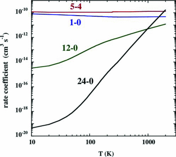
The rate coefficients for the collisional de‐excitation of SiO by H2, for the specified rotational transitions, J→J− 1. The data, which derive from the collision calculations of Dayou & Balança (2006) for T≤ 300 K, have been extrapolated to T= 2000 K.
The consequences for the SiO line intensities and line profiles of using the rate coefficients that have been extrapolated to T= 2000 K are illustrated in Figs A2 and A3, respectively. The initial increase in the kinetic temperature of the gas in the shock wave results in significant emission from the SiO levels of high excitation, owing to the rapid rise in the rates of collisional transitions directly to these levels from low‐lying rotational states, which have relatively high population densities. On the other hand, if it is assumed that the rate coefficients for all de‐excitation transitions remain constant for T≥ 300 K, as in G08a,b, the emission from the levels of high excitation is much weaker: see Fig. A2. Furthermore, the contribution to the line profiles from the region in which the kinetic temperature is rising and the gas is being accelerated is suppressed: see Fig. A3. Of course, the assumption that the rate coefficients remain constant at high temperatures is itself an approximation, but one that has the advantage of eliminating the non‐physical behaviour is described here.
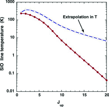
A comparison of the intensities of SiO lines, arising from the rotational levels Jup, for a C‐type shock wave model of speed vs= 25 km s−1, pre‐shock gas density nH= 104 cm−3 and initial magnetic field strength B= 100 μG, calculated using collisional de‐excitation rate coefficients that were either extrapolated (blue curve) or assumed to remain constant for T≥ 300 K (red curve).
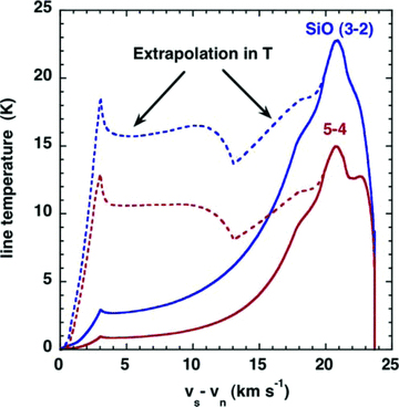
A comparison of the J= 3 → 2 and 5 → 4 SiO line profiles for a C‐type shock wave model of speed vs= 25 km s−1, pre‐shock gas density nH= 104 cm−3 and initial magnetic field strength B= 100 μG, calculated using collisional de‐excitation rate coefficients that were either extrapolated (broken curves) or assumed to remain constant for T≥ 300 K (full curves).
APPENDIX B: INFLUENCE OF THE GRAIN‐SIZE DISTRIBUTION ON LINE PROFILES
The size distribution of the grains can have significant effects on the thermal profile of the shock wave and the gas‐phase chemistry in the models. The results presented above were obtained with the size distribution of Mathis et al. (1977; ‘MRN distribution’), adopting upper and lower limits to the grain radius 0.3 ≥ag≥ 0.01 μm; the fractional abundance of the PAH in the gas phase was taken to be nPAH/nH= 10−6. We have also considered an alternative scenario of large, single‐size grains of radius ag= 0.5 μm. In this case, it was assumed that the PAH had agglomerated with the grains and hence were absent from the gas phase. The thermal profiles of models of shock waves with speeds 10 ≤vs≤ 40 km s−1, pre‐shock density nH= 2 × 104 cm−3 and magnetic field strength B= [nH(cm −3)]0.5 μG, obtained under these two different assumptions regarding the grain‐size distribution, are compared in Fig. B1.
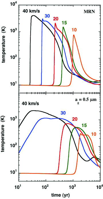
A comparison of the thermal profiles of C‐type shock wave models of the specified speeds, calculated with either the grain‐size distribution of Mathis et al. (1977; MRN), for grain radii 0.3 ≥ag≥ 0.01 μm or single‐size grains of radius ag= 0.5 μm. The pre‐shock gas density is nH= 2 × 104 cm−3 and the initial magnetic field strength is B= 141 μG.
As indicated in Section 2.3, the ‘large’ grains result in a wider and flatter thermal profile, with a lower maximum temperature, as may be seen in Fig. B1. These changes, to the thermal balance and the chemistry, are reflected in the CO and SiO integrated line intensities,4 plotted in Figs B2 and B3, respectively. It is remarkable that a modification of the grain‐size distribution alone can lead to such significant changes in the line intensities.
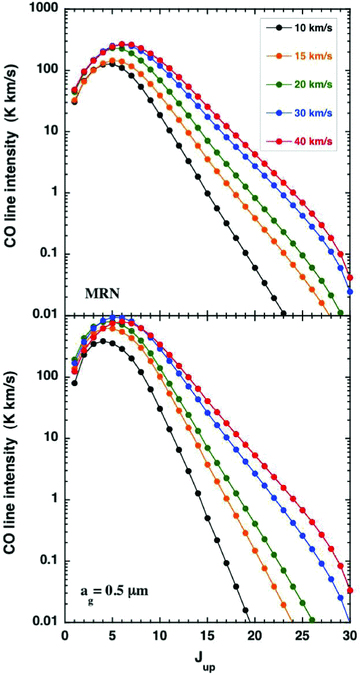
A comparison of the CO line intensities, TdV, for C‐type shock wave models of the specified speeds, calculated with either the grain‐size distribution of Mathis et al. (1977; MRN), for grain radii 0.3 ≥ag≥ 0.01 μm or single‐size grains of radius ag= 0.5 μm. The pre‐shock gas density is nH= 2 × 104 cm−3 and the initial magnetic field strength is B= 141 μG.
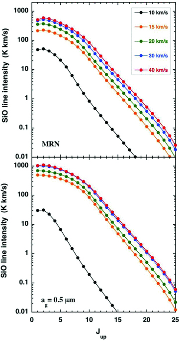
A comparison of the SiO line intensities, TdV, for C‐type shock wave models of the specified speeds, calculated with either the grain‐size distribution of Mathis et al. (1977; MRN), for grain radii 0.3 ≥ag≥ 0.01 μm or single‐size grains of radius ag= 0.5 μm. The pre‐shock gas density is nH= 2 × 104 cm−3 and the initial magnetic field strength is B= 141 μG.
Molecular hydrogen can be at least partially dissociated in shock waves, through collisions with H, He and H2. Molecules such as NH3 and H2O are, in turn, dissociated in collisions with the atomic hydrogen that is produced; the endothermicity of these dissociation reactions is higher for H2O (9265 K) than for NH3 (5170 K; see Table 1). The corresponding rates of collisional dissociation increase exponentially with the temperature of the neutral fluid and are proportional to the density of atomic hydrogen. Consequently, the degree of dissociation tends to increase with the shock speed and the pre‐shock gas density, other parameters being equal. However, the width of the shock wave, and hence the time of exposure of the molecules to the hot neutral fluid, is also significant. As may be seen from Fig. B1, this time is greater in the case of (large) single‐size grains than in the case of an MRN distribution of grain sizes. It follows that the relative abundance of NH3 and H2O varies with position in the shock wave, with the variation being most pronounced at high shock speeds and pre‐shock gas densities. This point is illustrated in Fig. B4, where we plot the ortho‐NH3 to ortho‐H2O, 572 GHz to 557 GHz, line ratio for both an MRN size distribution and single‐size grains.
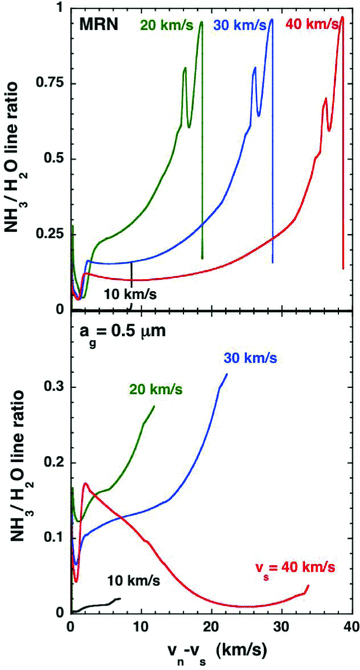
Plots of the 572 GHz ortho‐NH3 to the 557 GHz ortho‐H2O line ratio for C‐type shock wave models of the specified speeds, calculated with either the grain‐size distribution of Mathis et al. (1977; MRN), for grain radii 0.3 ≥ag≥ 0.01 μm or single‐size grains of radius ag= 0.5 μm. The pre‐shock gas density is nH= 2 × 104 cm−3 and the initial magnetic field strength is B= 141 μG.
The integrated line intensities of CO, SiO, and selected transitions of H2O and NH3, are provided for C‐type shock waves of speeds 10 ≤vs≤ 40 km s−1, nH= 2 × 104 cm−3 and B= 141 μG, for the two cases of an MRN size distribution and single‐size (ag= 0.5 μm) grains, in the online Supporting Information.
SUPPLEMENTARY MATERIAL
Additional Supporting Information may be found in the online version of this paper:
The integrated line intensities of CO, SiO and selected transitions of H2O and NH3, for C-type shock waves.
Please note: Wiley-Blackwell are not responsible for the content or functionality of any supporting materials supplied by the authors. Any queries (other than missing material) should be directed to the corresponding author for the article.
