


Abstract
With the aim of investigating galaxies with two strong simultaneous starbursts, we have extracted a sample of galaxies with double-peaked emission lines in their global spectra from the Sloan Digital Sky Survey (SDSS) spectral data base. We then fitted the emission lines Hα, Hβ, [O iii]λ5007, [N ii]λ6584, [S ii]λ6717 and [S ii]λ6731 of 129 spectra by two Gaussians to separate the radiation of the two (blue and red) components. A more or less reliable decomposition of all these emission lines has been found for 55 spectra. Using a standard Baldwin, Phillips & Terlevich (BPT) classification diagram, we have been able to divide the galaxies from our sample into two subsamples: Sample A consisting of 18 galaxies where both components belong to the photoionized class of objects, and Sample B containing 37 galaxies that show non-thermal ionization [active galactic nuclei (AGNs)]. We have examined the properties of the blue and red components, and found that the differences between radial velocities of components lie within 200–400 km s−1 for galaxies of both subsamples. The equivalent number of ionizing stars is in the range of 104–105 O7V stars for each component in the galaxies of Sample A. We have estimated the oxygen and nitrogen abundances as well as the electron temperatures for each component using the recent NS-calibration and from global spectra for galaxies from Sample A using both NS- and ON-calibration. We have found that the global oxygen abundance is typically in between the measured abundances of individual components for our sample of galaxies, and that both calibrations provide consistent global abundances. Finally, we suggest that the classical O/H–N/O diagram be used to test the reliability of the dividing lines between starburst-like objects and AGNs in the so-called BPT diagram.
1 INTRODUCTION
The study of starburst galaxies is very important for understanding both star formation and (chemical) evolution of galaxies. The Sloan Digital Sky Survey (SDSS, York et al. 2000) provides a very large data base of spectra of galaxies, which has been used in many studies of the chemical evolution of galaxies (see, e.g. Izotov et al. 2004; Kniazev et al. 2004; Tremonti et al. 2004; Pilyugin & Thuan 2007, 2011; Thuan, Pilyugin & Zinchenko 2010).
The SDSS spectra are obtained through 3-arcsec diameter fibres. At a redshift of z = 0.12 (which is the mean value of the redshifts of galaxies considered at the present study), the projected aperture diameter is ∼7 kpc. This suggests that the SDSS spectra of the considered galaxies are closer to global spectra (composite nebulae that include multiple star clusters), rather than to spectra of individual H ii regions. In a typical case, many individual H ii regions are distributed over the disc of a galaxy. Due to the rotation of galaxies, H ii regions will have different radial velocities depending on the inclination of their host galaxy. One may expect that the emission line profile in the global SDSS spectra of such composite nebulae in distant galaxies can be described by a Gaussian which is wider than that for an individual H ii region. If two strong starbursts take place in a galaxy and the giant H ii regions associated with those starbursts make a dominant contribution to the radiation in the emission lines then one could expect a double-peaked emission line profile in the global spectrum of the galaxy. While double-peaked emission lines have been extensively studied in active galactic nuclei (AGNs) and radio galaxies, double-starburst galaxies are as yet unexplored. These systems may induce errors in abundance determinations due to the mixing of two starburst events. Then, establishing the abundances for each component and the global abundances (using the ‘global flux’ in every emission line as the sum of fluxes from the blue and red components) will shed light on the impact of the double-peaked emission lines on global abundance determinations. To this aim, we have carried out a search for SDSS spectra of galaxies with double-peaked emission line profiles, revealing several hundred candidates where two strong starbursts can be observed simultaneously.
Here, we separate the radiation of two giant H ii regions associated with two different starbursts by the fitting of two Gaussians to the emission lines in the global spectra. We examine the properties of each component of these ‘binary starbursts’: the electron density, the oxygen and nitrogen abundances, and the number of ionizing stars they contain. These objects also provide an additional possibility to test how representative abundances derived from global spectra are for the whole galaxies. A comparison between oxygen abundances in the blue and red components and global oxygen abundances will tell us something about the reliability of the abundances derived from global spectra. We test the reliability of global abundances by comparison of global abundances obtained using two recent strong-line calibrations as well.
Finally, we suggest the use of the classical O/H–N/O diagram to test the credibility of the dividing lines between the starburst-like objects and the AGNs in the Baldwin, Phillips & Terlevich (1981) (BPT) classification diagram.
The paper is organized as follows. Decomposition of the double-peaked emission line profiles in the global SDSS spectra and the selection of galaxies are described in Section 2. The general properties of the selected sample of galaxies are given in Section 3. The oxygen and nitrogen abundances and the electron temperatures derived for individual (blue or red) components and from global spectra are discussed in Section 4, and Section 5 gives a brief summary of the main results.

The electron temperatures t are given in units of 104 K.
2 THE DATA
As the first step, we have extracted several hundred spectra of galaxies with double-peaked emission lines from data release 7 (Abazajian et al. 2009) of the Sloan Digital Sky Survey (SDSS). In our previous work we visually inspected SDSS spectra aiming to search for spectra where the two auroral lines [O iii]λ4363 and [N ii]λ5755 can be detected simultaneously (Pilyugin et al. 2010). We have also collected spectra with double-peaked emission lines. Although we have considered all the SDSS DR7 spectra, we do not suggest that our sample of SDSS spectra with double-peaked emission lines is exhaustive.
 on the interval corresponding to differences between radial velocities of the blue and red components from 120 to 600 km s−1. This range was divided into 160 intervals Δλi with a step of 3 km s−1. The best-fitting parameters for every interval of Δλi are derived by finding the minimum of the mean difference,
between the measured flux fobs(λk) and the flux f(λk) given by equation (8) on the wavelength interval between λa and λb. The ‘true’ values of  ,
,  ,
,  ,
,  ,
,  and
and  are then selected by comparing the minimum values of εi for different intervals of Δλi. In other words, we have used a two-step procedure to obtain the best-fitting parameters.
The fit to the [O iii]λ5007 line is obtained using the wavelength interval from λa= 4982 Å to λb= 5032 Å. The continuum flux fc is assumed to be constant between λa= 6523 Å and λb= 6608 Å in fitting of the Hα and [N ii]λ6584 lines, and between λa= 6690 Å and λb= 6760 Å in fitting of the [S ii]λ6717 and [S ii]λ6731 lines. The fits to the Hα, Hβ, [O iii]λ5007, [N ii]λ6584, [S ii]λ6717 and [S ii]λ6731 lines in the spectra (spSpec 280 51612 635) of the SDSS object J112655.58+004047.0 are shown in Fig. 1.
![The observed spectrum of the SDSS object J112655.58+004047.0 (spSpec 280 51612 635) and double-Gaussian fits to the emission lines Hβ, [O iii]λ5007, Hα, [N ii]λ6584, [S ii]λ6717 and [S ii]λ6731. The solid line is the observed line profile. The long-dashed (blue) lines are the profiles of the blue and red components, respectively, and the short-dashed (red) line is the sum of the blue and red components. A colour version of this figure is available in the online version.](https://oup.silverchair-cdn.com/oup/backfile/Content_public/Journal/mnras/419/1/10.1111_j.1365-2966.2011.19714.x/1/m_mnras0419-0490-f1.jpeg?Expires=1750202396&Signature=yVEaJeQRsw4ozKrZGgTFjaOaDQb-R1WejbxopiXCuwpmlCrMSs8kOZBb6k62uNgtpjihmZbw8ux97KDhMGnjUnZ4t47xYYvmpp5qgHRC0JBhBddVKh4Vq2EjyP0lfUhJWTJ6h0-LzKalZ6hXoa4t~sIbVwNyxNcwb15vJEWTTdtIOf-6AmsD6bzU-jDdkORfG5UR0jK6FoBBacZoXV9yEGlfpFlUweB-Yp1E0kwX3M6bptJwUQi-h2bvoO0IsFJ31Yb3PQCmtbopQ~h0L-jnX7aFjgpwnW0JeBrPiJktdXr5hB~cTEf5p7Gu9yV3w74P~bYwbruaBCKNOuYEFJWHRQ__&Key-Pair-Id=APKAIE5G5CRDK6RD3PGA)
The observed spectrum of the SDSS object J112655.58+004047.0 (spSpec 280 51612 635) and double-Gaussian fits to the emission lines Hβ, [O iii]λ5007, Hα, [N ii]λ6584, [S ii]λ6717 and [S ii]λ6731. The solid line is the observed line profile. The long-dashed (blue) lines are the profiles of the blue and red components, respectively, and the short-dashed (red) line is the sum of the blue and red components. A colour version of this figure is available in the online version.
We have found 129 spectra where a double-Gaussian fit can be obtained for each emission line. Unfortunately, the value of the parameter ε given by equation (9) cannot serve as an effective criterion for selecting spectra with reliable decompositions. First of all, the value of ε is a measure of the quality of the double-Gaussian fit to the global line profiles rather than a measure of the quality of the decomposition. In addition, the observed double-peaked line profiles are covered by about 10 wavelength points only at the SDSS spectroscopic resolution. Hence, the value of ε may be affected significantly by the noise from just one data point. Therefore we have selected spectra where the decomposition of the blue and red components for each emission line seems to be reliable, based upon visual inspection of the double-Gaussian fits (how well a double-peak is seen in each emission line), taking into account the limited quality of the SDSS spectra. Our final list contains 55 spectra. Certainly, our selection is somewhat subjective, but as for the spectra excluded from further consideration here, the only lines that cannot be reliably decomposed into two components are [S ii]λ6717 or/and [S ii]λ6731. The other lines can be fitted rather well by two Gaussians. Even if the [S ii]λ6717 and [S ii]λ6731 lines will not be used as separate lines in most of this study, we have used the fits to these lines as a test of the robustness of the sample.
Since measurements of the [N ii]λ6584 and [O iii]λ5007 lines are more reliable than those of the [N ii]λ6548 and [O ii]λ4959 lines, we have used equation (6) to obtain the value of N2 and equation (5) to determine the value of R3.
The measured emission fluxes F have been corrected for interstellar reddening. We have obtained the extinction coefficient C(Hβ) using the theoretical Hα-to-Hβ ratio (=2.86) and the analytical approximation to the Whitford interstellar reddening law by Izotov, Thuan & Lipovetsky (1994).
The redshift z and stellar mass MS of each galaxy were taken from the MPA/JHU catalogues.2 The techniques used to construct the catalogues are described in Brinchmann et al. (2004), Tremonti et al. (2004) and other publications of those authors.
3 GENERAL PROPERTIES OF THE SELECTED STARBURSTS
3.1 BPT classification diagram
The intensities of strong, easily measured lines can be used to separate different types of emission-line objects according to their main excitation mechanism (i.e. starburst or AGN). Baldwin et al. (1981) proposed a diagram (BPT classification diagram) where the excitation properties of H ii regions are studied by plotting the low-excitation [N ii]λ6584/Hα line ratio against the high-excitation [O iii]λ5007/Hβ line ratio. Using the BPT classification diagram, we have divided all galaxies from our sample into two subsamples. The first subsample (A) consists of 18 galaxies where both components (blue and red) are starburst-like objects. The galaxies in Sample A are listed in Table 1. The second subsample (B) contains 37 galaxies where one or both components show non-thermal ionization (here referred to as AGNs). It should be noted that all components, in all galaxies, in our sample have narrow lines regardless of their positions in the [N ii]λ6584/Hα versus [O iii]λ5007/Hβ diagram.
Oxygen and nitrogen abundances and electron temperatures of individual components as well as global values of Sample A.
| SDSS numbera | Spectrum numberb | 12+log(O/H)blueNS | 12+log(O/H)redNS | 12+log(N/H)blueNS | 12+log(N/H)redNS | tblueNS | tredNS |
| 12+log(O/H)globNS | 12+log(O/H)globON | 12+log(N/H)globNS | 12+log(N/H)globON | tglobNS | tglobON | ||
| J015847.30−101802.7 | 665 52168 018 | 8.41 | 8.45 | 7.44 | 7.37 | 0.89 | 0.87 |
| 8.43 | 8.45 | 7.41 | 7.45 | 0.88 | 0.86 | ||
| J084845.58+542329.1 | 446 51899 595 | 8.47 | 8.24 | 7.69 | 6.85 | 0.80 | 1.06 |
| 8.41 | 8.44 | 7.47 | 7.55 | 0.90 | 0.87 | ||
| J091911.35+531424.0 | 553 51999 639 | 8.48 | 8.50 | 7.67 | 7.57 | 0.80 | 0.79 |
| 8.49 | 8.46 | 7.63 | 7.46 | 0.80 | 0.83 | ||
| J103007.07+412353.5 | 1360 53033 186 | 8.30 | 8.41 | 6.95 | 7.15 | 1.00 | 0.96 |
| 8.37 | 8.42 | 7.07 | 7.25 | 0.97 | 0.95 | ||
| J103404.17+061210.2 | 999 52636 150 | 8.22 | 8.16 | 6.85 | 6.71 | 1.09 | 1.12 |
| 8.20 | 8.24 | 6.77 | 6.89 | 1.11 | 1.09 | ||
| J103822.61+505814.7 | 1009 52644 042 | 8.48 | 8.42 | 7.70 | 7.47 | 0.80 | 0.87 |
| 8.45 | 8.45 | 7.59 | 7.55 | 0.83 | 0.84 | ||
| J104137.27+103252.0 | 1600 53090 020 | 8.52 | 8.61 | 7.98 | 7.97 | 0.74 | 0.69 |
| 8.57 | 8.57 | 7.99 | 7.97 | 0.71 | 0.72 | ||
| J112655.58+004047.0 | 280 51612 635 | 8.49 | 8.42 | 7.73 | 7.53 | 0.78 | 0.86 |
| 8.46 | 8.44 | 7.64 | 7.55 | 0.82 | 0.83 | ||
| J113122.19−005606.4 | 281 51614 007 | 8.41 | 8.37 | 7.47 | 7.20 | 0.89 | 0.93 |
| 8.39 | 8.41 | 7.33 | 7.36 | 0.91 | 0.89 | ||
| J113413.84+533601.2 | 1014 52707 096 | 8.41 | 8.15 | 7.31 | 6.70 | 0.92 | 1.12 |
| 8.41 | 8.45 | 7.15 | 7.23 | 0.94 | 0.95 | ||
| J113515.65+234606.0 | 2501 54084 010 | 8.40 | 8.32 | 7.12 | 6.93 | 0.87 | 0.99 |
| 8.39 | 8.45 | 7.09 | 7.18 | 0.91 | 0.90 | ||
| J113835.63+281801.1 | 2220 53795 089 | 8.41 | 8.33 | 7.42 | 6.95 | 0.89 | 0.90 |
| 8.41 | 8.41 | 7.32 | 7.26 | 0.90 | 0.90 | ||
| J114234.66−030527.9 | 329 52056 320 | 8.42 | 8.33 | 7.38 | 6.97 | 0.87 | 0.97 |
| 8.37 | 8.43 | 7.06 | 7.13 | 0.93 | 0.93 | ||
| J124844.42+250522.6 | 2661 54505 412 | 8.43 | 8.55 | 7.59 | 8.01 | 0.83 | 0.72 |
| 8.47 | 8.44 | 7.73 | 7.58 | 0.80 | 0.82 | ||
| J132253.24+585942.2 | 959 52411 397 | 8.46 | 8.54 | 7.64 | 7.86 | 0.82 | 0.73 |
| 8.50 | 8.47 | 7.76 | 7.59 | 0.77 | 0.80 | ||
| J141439.58+033601.8 | 583 52055 137 | 8.38 | 8.47 | 7.44 | 7.66 | 0.89 | 0.80 |
| 8.42 | 8.44 | 7.54 | 7.56 | 0.84 | 0.83 | ||
| J142504.46+050556.7 | 584 52049 571 | 8.45 | 8.43 | 7.63 | 7.44 | 0.82 | 0.88 |
| 8.44 | 8.42 | 7.54 | 7.45 | 0.85 | 0.87 | ||
| J161555.12+420624.5 | 1171 52753 376 | 8.51 | 8.38 | 7.40 | 7.08 | 0.89 | 0.96 |
| 8.48 | 8.50 | 7.33 | 7.45 | 0.91 | 0.90 |
a The objects are listed in order of right ascension; b the spectrum number consists of the SDSS plate number, the modified Julian date of the observation, and the number of the fibre on the plate.
The theoretical Hα-to-Hβ ratio for thermally photoinized nebulae has been used for dereddening of measured emission lines in both subsamples. The application of the same dereddening algorithm to all objects can be justified as follows. The parameters which are dependent on the absolute fluxes are analysed in the present study only for the starburst-like objects (where this dereddening algorithm is correct). As for the AGNs, this dereddening algorithm can introduce an appreciable error in the dereddened line intensities. However, the dereddened line intensities in the AGNs serve only for classification of these objects. The wavelengths of the N ii]λ6584 and Hα lines (as well [O iii]λ5007 and Hβ) are very similar and, consequently, the [N ii]λ6584/Hα- and [O iii]λ5007/Hβ-line ratios are not that sensitive to the dereddening algorithm. Therefore, the adopted dereddening algorithm does not result in a significant shift of the position of the object in the [N ii]λ6584/Hα versus [O iii]λ5007/Hβ diagram and is not likely to result in misclassification of objects.
from Kewley et al. (2001). The lower panel in Fig. 2 shows the global data. The grey (in the printed version – light-blue in the colour version) filled circles show a large sample of SDSS emission-line galaxies from Thuan et al. (2010). The dark (black) filled circles show our sample of SDSS galaxies with double-peaked emission lines (global spectra, sum of blue and red components). The lines are the same as in the upper panel. We choose here to use the separation line from Kauffmann et al. (2003) (see below, Section 4).
![The [N ii]λ6584/Hα versus [O iii]λ5007/Hβ diagram. Upper panel: the open (blue) circles are the blue components and the (red) plus signs are the red components of the photoionized objects. The open (blue) squares are the blue components and the (red) crosses are the red components of the AGNs. The solid line separates objects with H ii spectra from those containing an AGN according to Kauffmann et al. (2003), while the dashed line is the same according to Kewley et al. (2001). Lower panel: the grey (light-blue) filled circles show a large sample of emission-line SDSS galaxies from Thuan et al. (2010). The dark (black) filled circles show our sample of SDSS galaxies with double-peaked emission lines (global spectra, sum of blue and red components). A colour version of this figure is available in the online version.](https://oup.silverchair-cdn.com/oup/backfile/Content_public/Journal/mnras/419/1/10.1111_j.1365-2966.2011.19714.x/1/m_mnras0419-0490-f2.jpeg?Expires=1750202396&Signature=tY9cU7hXbcQuKd5erB88atmt5R5dhuPSID8f8JOf740C4CSuoTNDXHmyNlhOBIGLUnf2VU23w-jtWt8wUyfEngyQVP6QTNk6MxN9LLDZH4R-WycQfPxNdK40o1fbpbLzjf-CUoqZijC1~D1nQZM8oObm1EQD1UyP75sFrdA5rl7C8DoO9pjYXYTZJR3nKl-HbHixQblgOtGhZHfEIaz3DT8DMZ0UZN3PbRzHZZSzBY43fcJWed3Z0TNH0gvXIVtx-V7PmVqGpxrPYni9oHofgqrlmboX~otjts-15SFWfuJKl3PGP4u9mEo-0BykXGokEboW7kR1xoAhenn663PByg__&Key-Pair-Id=APKAIE5G5CRDK6RD3PGA)
The [N ii]λ6584/Hα versus [O iii]λ5007/Hβ diagram. Upper panel: the open (blue) circles are the blue components and the (red) plus signs are the red components of the photoionized objects. The open (blue) squares are the blue components and the (red) crosses are the red components of the AGNs. The solid line separates objects with H ii spectra from those containing an AGN according to Kauffmann et al. (2003), while the dashed line is the same according to Kewley et al. (2001). Lower panel: the grey (light-blue) filled circles show a large sample of emission-line SDSS galaxies from Thuan et al. (2010). The dark (black) filled circles show our sample of SDSS galaxies with double-peaked emission lines (global spectra, sum of blue and red components). A colour version of this figure is available in the online version.
Fig. 2 shows that in the majority of cases both components belong either to starburst-like objects or to double-peaked AGNs. There seems to be a strong selection effect. Indeed the requirement that a reliable double-Gaussian fit can be obtained for each of the emission lines is satisfied for spectra with SDSS resolution only in cases when the contributions of the blue and red components are similar. As a result, our sample contains galaxies with similar [N ii]λ6584/Hα and [O iii]λ5007/Hβ fluxes for both components. Consequently, both components lie close to each other in the [N ii]λ6584/Hα versus [O iii]λ5007/Hβ diagram.
3.2 Velocity separation
Fig. 3 shows the difference between radial velocities of the blue and red components as a function of stellar mass (upper panel) and of redshift (lower panel). The open circles show galaxies from Sample A, while the plus signs show galaxies from Sample B. The difference between the radial velocities of the blue and red components is determined from the mean value of the differences for individual lines. The scatter is typically a few per cent, but less than 10 per cent in all the cases. Fig. 3 shows that this difference between the radial velocities ranges between 200 and 400 km s−1, and that it does not correlate with stellar mass, nor with redshift. However, the upper panel of Fig. 3 shows that the galaxies with AGN-like spectra are more massive, on average, than the galaxies with starburst-like spectra. This agrees with the conclusion by Kauffmann et al. (2003) that AGNs reside almost exclusively in massive galaxies.
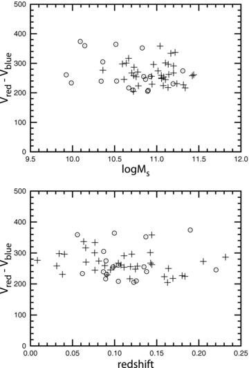
The difference between radial velocities of blue Vblue and red Vred components (in units of km s−1) as a function of the stellar mass of a galaxy (upper panel) and of redshift (lower panel). The open circles show galaxies from Sample A. The plus signs show galaxies from Sample B.
Here we will discuss the velocity separations of the double peaks and the Gaussian width parameters of the Hβ lines. It was noted above that the only lines that cannot be reliably decomposed into two components are [S ii]λ6717 or/and [S ii]λ6731 while the other lines can be fitted rather well by two Gaussians in 129 selected galaxies. Hence, all the 129 galaxies will be included in this particular discussion. The lower-limit difference between the radial velocities of the blue Vblue and red Vred components (∼200 km s−1) in our sample of galaxies is defined by the requirement that the two peaks in the line profile should be clearly separated. Smith et al. (2010) have selected AGNs from SDSS having double-peaked profiles of [O ii]λ4959, 5007 and other narrow emission lines by visual inspection of the quasar spectra. The lower-limit velocity separation of the double peaks in their sample is also around 200 km s−1, i.e. similar to that in our sample of galaxies.
The rotation velocity of large spiral galaxies is usually above 200 km s−1 and can reach about 300 km s−1 (see the compilation by Pilyugin, Vílchez & Contini 2004). The difference between the radial velocities of two H ii regions in a spiral galaxy with a large inclination can thus be around 400–600 km s−1. As an alternative interpretation, the large difference between radial velocities of blue and red components can be if components are parts of two merging systems. The largest difference between radial velocities of the blue and red components (∼400 km s−1) in our sample of galaxies is well within the range given above. One may expect that in the case where many individual H ii regions are distributed over the disc of a giant spiral galaxy with a large inclination, the emission line profile in the global single-peaked SDSS spectra of such composite nebulae can have a similar width.
3.3 Gaussian linewidth
We have extracted the linewidth of the Hβ line (σHβ) for 255 539 emission-line galaxies (with equivalent widths of the Hβ and Hα lines EW(Hβ) > 1.5, EW(Hα) > 1.5, and 2σHβ < 600 km s−1) from the SDSS data base. It should be noted that a single-Gaussian fit to the double-peaked emission line can be bad even as a first-order approximation (Fig. 4).
![The approximation of the observed Hβ line profile [dark (black) curve] by the single [long-dashed (red) curve] and two [short-dashed (blue) curve] Gaussians in the spectra of three galaxies from Sample A. A colour version of this figure is available in the online version.](https://oup.silverchair-cdn.com/oup/backfile/Content_public/Journal/mnras/419/1/10.1111_j.1365-2966.2011.19714.x/1/m_mnras0419-0490-f4.jpeg?Expires=1750202396&Signature=Y4YDaX7EjF69HRYizAKsg8qzzyAc17keN63vBlHc-n7sYaOvyiOpq9l5ke52BW6c43B07A~QZaxRfgpG5gEyJKwa1QAWitPofMJzCoMd-RFuGk3Od89Priscipo4mc9A3TXzPZSDwmLOwD5IV3lDU9A6CNIOc3tOvXfR~m7jXnbBPfjTMsSBWBxW-kq6yII64lWS6nSDdQ15P~SfYx4Dw8rl9UbvWBD8z2dsM4lqraKCu-HhlFchNflHn9hmaD3JGibE9XyDT3hqx3nyO4cYf4cJXSpRsD3DApW~EAlWssV1G1BDbncuwRPmPs1ULk5usMgBokINVusT2RKulpsCfg__&Key-Pair-Id=APKAIE5G5CRDK6RD3PGA)
The approximation of the observed Hβ line profile [dark (black) curve] by the single [long-dashed (red) curve] and two [short-dashed (blue) curve] Gaussians in the spectra of three galaxies from Sample A. A colour version of this figure is available in the online version.
Fig. 5 shows the Gaussian width parameter σHβ (in units of km s−1) as a function of redshift for a large sample of emission-line galaxies extracted from SDSS [grey (blue) filled circles], for the global spectra of the selected 129 SDSS galaxies with double-peaked emission lines [dark (black) filled circles], and for the blue and red components of those galaxies [open (red) triangles]. The values of the Gaussian width parameter σHβ for the global spectra (including our sample of 129 galaxies) were taken from the SDSS data base and measured for the blue and red components. Fig. 5 shows that the linewidths of the majority of the blue and red components in our sample of galaxies are within the range from ∼140 to ∼220 km s−1 and they occupy the same area as the majority of emission-line galaxies from SDSS. However, several components have larger widths, up to ∼300 km s−1. This suggests that some components can themselves be composite nebulae. The Gaussian width parameters of the global spectra of our sample of galaxies are situated above and along the upper envelope defined by the emission-line galaxies from SDSS. However, some of them are situated in the same region as the majority of the blue and red components. These are galaxies where the intensities of the blue and red components differ significantly. In such a case the single-Gaussian fit to the double-peaked emission line alone reproduces the strongest component as can be seen in the lower panel of Fig. 4. Thus, the large Gaussian width parameters of the global spectra cannot be a reliable criterion for selecting candidates for galaxies with double-peaked emission lines. Using this criterion, one will simply miss the galaxies where the intensities of the blue and red components differ significantly.
![The Gaussian width parameter (in units of km s−1) as a function of redshift for emission-line galaxies taken from SDSS [grey (blue) filled circles], for global spectra of the selected 129 SDSS galaxies with double-peaked emission lines [dark (black) filled circles], and for the blue and red components of those galaxies [open (red) triangles]. A colour version of this figure is available in the online version.](https://oup.silverchair-cdn.com/oup/backfile/Content_public/Journal/mnras/419/1/10.1111_j.1365-2966.2011.19714.x/1/m_mnras0419-0490-f5.jpeg?Expires=1750202396&Signature=CxhViWhz4SHp4ChcKVW-bd607rrXGaKYkrw7o4qu-vlwlsQwPhAC9Ml09nft239HTo4Vvw9-tB~6D1~Rig8hFBO0a~Dc1m~u0Dt-l3tg2MJOhGm3A5UJlLX0a7Yw2URCaF885bvYWGGQ7tj3TWUZaYKE5E9gHaBllbPZ4RnmcKVgYIaToiGHzHa17Asl5SomQSmS8ijv6HCnFAG1R4DEE7SEP3Ye6z0r90~hrNUtFPue6Y5z52rGVk8jI7I7zjtx7Pedum4lXZ3xdkziuTlCm4gqk5tDCKMxj2bdDjMBZ7OnpWw0Fqzb136ffXVPjESFw3eWw1lQISjJ-dZjtOTC4A__&Key-Pair-Id=APKAIE5G5CRDK6RD3PGA)
The Gaussian width parameter  (in units of km s−1) as a function of redshift for emission-line galaxies taken from SDSS [grey (blue) filled circles], for global spectra of the selected 129 SDSS galaxies with double-peaked emission lines [dark (black) filled circles], and for the blue and red components of those galaxies [open (red) triangles]. A colour version of this figure is available in the online version.
3.4 Starburst strength
An important characteristic of an H ii region is the number of ionizing stars it contains. Under the assumption of an ionization-bounded and dust-free nebula, the Hβ luminosity provides an estimate of the ionizing flux. The ionizing flux can be expressed in terms of the number of so-called equivalent O stars of a given subtype responsible for producing the ionizing luminosity. The number of zero-age main-sequence O7V stars, NO7V, is usually used to specify the ionizing flux. The value of NO7V can be easily derived from the observed Hβ luminosity and the Lyman continuum flux of an individual O7V star. The number of ionizing photons from an O7V star is NLc= 5.62 × 1048 s−1 (Martins, Schaerer & Hillier 2005) or NLc= 1.12 × 1049 s−1 (Vacca 1994). Here the value of NLc from Martins et al. (2005) has been adopted. If we instead adopt the value of NLc from Vacca (1994), the number of equivalent O stars increases by about a factor of 2. One ionizing photon from the star produces 0.157 Hβ photons (0.449 Hα photons) from the H ii region (Osterbrock & Ferland 2006). The density-bounded dust-free H ii region excited by one O7V star will have the Hβ luminosity 3.38 × 1036 erg s−1 or  and the Hα luminosity 7.64 × 1036 erg s−1 or
  . When these conditions (density-bounded and/or dust-free) are not met, the values of the number of equivalent O stars obtained here should be interpreted as lower limits.
 is obtained from the observed
  flux using the relation (Blagrave et al. 2007)
where C(Hβ) is the extinction coefficient.

where d is the distance in Mpc, c the speed of light in km s−1, and z the redshift. H0 is the Hubble constant, here assumed to be equal to 72 (±8) km s−1 Mpc−1 (Freedman et al. 2001). Since objects from Sample A have low redshifts (only two objects have z > 0.15) the low-redshift approximation for distance determination has been used.
The upper panel of Fig. 6 shows the equivalent number of O7V stars NO7V responsible for the excitation of blue and red components in galaxies from Sample A. The lower panel shows the ratio of equivalent numbers of O7V stars responsible for the excitation of blue and red components. An inspection of Fig. 6 shows that the typical value of the equivalent number of O7V stars in starbursts in galaxies from Sample A is in the range of 104–105. Kennicutt (1988) has given the mean Hα fluxes for the three brightest H ii regions in a sample of nearby galaxies. Those fluxes, converted to equivalent numbers of O7V stars, correspond to NO7V∼ 102. Thus, both the blue and red components in our sample of SDSS galaxies contain many more (up to 2–3 orders of magnitude) ionizing stars, when compared to the brightest H ii regions in nearby galaxies. Fig. 7 shows a comparison of the equivalent number of O7V stars, NO7V, for Sample A (the sum of the NO7V for blue and red components) and for a large sample of star-forming galaxies from SDSS. This sample of galaxies was selected from the MPA/JHU catalogues using the dividing line between starburst-like objects and AGNs from Kauffmann et al. (2003). The reddening-corrected Hβ flux is obtained using equation (12). Only the galaxies with EW(Hβ) > 1.5 and EW(Hα) > 1.5 are shown. Fig. 7 also shows that the number of ionizing stars in the galaxies with two starbursts from our Sample A is similar to that of galaxies (from SDSS) with a large number of ionizing stars.
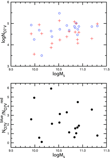
Upper panel: the equivalent number of O7V stars NO7V responsible for the excitation of H ii regions versus the host galaxy stellar mass for Sample A. The open (blue) circles show the blue components and the (red) plus signs show the red components. Lower panel: the ratio of equivalent numbers of O7V stars responsible for the excitation of the blue and red components. A colour version of this figure is available in the online version.
![The equivalent number of O7V stars NO7V responsible for the excitation of the H ii regions versus redshift for Sample A [dark (black) filled circles] and for star-forming galaxies taken from SDSS [grey (blue) filled circles]. A colour version of this figure is available in the online version.](https://oup.silverchair-cdn.com/oup/backfile/Content_public/Journal/mnras/419/1/10.1111_j.1365-2966.2011.19714.x/1/m_mnras0419-0490-f7.jpeg?Expires=1750202396&Signature=s~dYzL05WTJuA7Ac49wWQ~78v4X3GWzWZc0ehEbp8m3fzsiuWD0ccoG16SX854H9fZykOkhFc4jY~W3yCBSmqjHlnpEkDkhPFa~iryifgePwAKhIrQ3RIczbMcx4Thdp35WMEcj3uRm5wi3B3eswECejJ8KOEzTL4QKhSAYsweIdFH5karvP6xzCGqJhamG5VGLZx1zlGTKfJOt5jLrK3PYgZkq501ufmEgzUYetHKWgEjMegOHYzhgvTdTnaz9bIFfehbB-lYjhiSOq0KzYWm3JgyLGfRbWOEW4taIZrdelCV15vti0eOHR7dYHAfc5sT0I1z92K6OSUEx~gqZ81w__&Key-Pair-Id=APKAIE5G5CRDK6RD3PGA)
The equivalent number of O7V stars NO7V responsible for the excitation of the H ii regions versus redshift for Sample A [dark (black) filled circles] and for star-forming galaxies taken from SDSS [grey (blue) filled circles]. A colour version of this figure is available in the online version.
3.5 Electron density
Fig. 8 shows the density-sensitive [S ii]λ6717/[S ii]λ6731 line ratio as a function of the equivalent number of O7V stars, NO7V, in the starbursts. The open (blue) circles show the blue components. The (red) plus signs show the red components. The filled circles show the data from global spectra (sum of blue and red components). The expected zero density limit ([S ii]λ6717/[S ii]λ6731 = 1.44 at Ne=1 cm−3 with t2= 1.0) is shown by the solid line. The dashed and dotted lines show the line ratios corresponding to Ne=100 cm−3 ([S ii]λ6717/[S ii]λ6731 = 1.29) and Ne=200 cm−3 ([S ii]λ6717/[S ii]λ6731 = 1.18), respectively.
![The density-sensitive [S ii]λ6717/[S ii]λ6731 line ratio versus the equivalent number of O7V stars NO7V responsible for the excitation of H ii regions. The open (blue) circles show the blue components. The (red) plus signs show the red components. The filled circles show the sum of blue and red components. The solid line shows the zero-density limit (Ne=1 cm−3), the dashed line corresponds to the electron density Ne=100 cm−3, and the dotted line corresponds to the electron density Ne= 200 cm−3. A colour version of this figure is available in the online version.](https://oup.silverchair-cdn.com/oup/backfile/Content_public/Journal/mnras/419/1/10.1111_j.1365-2966.2011.19714.x/1/m_mnras0419-0490-f8.jpeg?Expires=1750202396&Signature=lnHGiWAVHcjSJfRNgUxb21R3SNvPAp7rDgxWe8Uxa7JadmlIhBB60SAAbWOxpkjtPlJ0KsCKDl8gE3TiUUXGiNLVwghuZDjhtAL859Vqs0EwBkABOdN6v3CowpQuxGZnjnlUXC5MQ0~2bVkraZNpozoCbf-ulKKc2bk00UBiR-g3EAV~AzCiPKE4XduQgK~TY-8vr~l-FFUg7KoFGTa~qGw375aF3eRWAP6EqYGhQh4N8TraL9WqjaXSEhYZdfhm2ShpYa5GrMmsRe5v3L1ek2r3XsUoRwUwkMv-wpP3s0mc3F4uVVOR0KiL1JUKKnbElVdxK7HX9T6e-FOul7sgNg__&Key-Pair-Id=APKAIE5G5CRDK6RD3PGA)
The density-sensitive [S ii]λ6717/[S ii]λ6731 line ratio versus the equivalent number of O7V stars NO7V responsible for the excitation of H ii regions. The open (blue) circles show the blue components. The (red) plus signs show the red components. The filled circles show the sum of blue and red components. The solid line shows the zero-density limit (Ne=1 cm−3), the dashed line corresponds to the electron density Ne=100 cm−3, and the dotted line corresponds to the electron density Ne= 200 cm−3. A colour version of this figure is available in the online version.
The density-sensitive [S ii]λ6717/[S ii]λ6731 line ratio in the global spectra of all the galaxies in our Sample A shows an electron density  cm−3 (filled circles in Fig. 8), with the majority of them having
  cm−3. Hence, they are all in the low-density regime, as is typical of the majority of extragalactic H ii regions (Zaritsky, Kennicutt & Huchra 1994; Bresolin et al. 2005; Gutiérrez & Beckman 2010). The [S ii]λ6717/[S ii]λ6731 line ratio in the blue and red components shows a larger scatter (see Fig. 8), which may be caused by the uncertainties in the line decomposition.
Two giant H ii regions located at different positions inside the disc (one H ii region can be associated with the circumnuclear star formation) may be responsible for the double-peaked emission lines in Sample A. However, the double-peaked emission lines in global spectra can be caused not only by two starbursts in the same galaxy, but also by two starbursts in two different galaxies, provided these galaxies are very closely located in the sky (projected on top of each other and thus detected within the same SDSS fibre). If the radiation from a star-forming region in a more distant galaxy passes through a less distant galaxy, one may expect that the extinction of the red component (star-forming region in the more distant galaxy) should be larger than the extinction of the blue component (star-forming region in the less distant galaxy). Fig. 9 shows the extinction coefficient C(Hβ) in the blue component versus the C(Hβ) in the red component for galaxies in Sample A. Fig. 9 also shows that there is no systematic difference between the values of the extinction coefficient C(Hβ) in the blue and red components. It should be noted, however, that the more distant galaxies can have slightly lower radial velocities than the less distant ones due to the random component of their radial velocities.
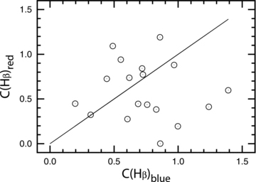
The extinction C(Hβ) in the blue component versus the extinction C(Hβ) in the red component for galaxies from Sample A.
4 ABUNDANCES AND TEMPERATURES
It is impossible to divide the [O ii]λ3727+λ3729 doublet into a blue and a red component at the SDSS spectral resolution. Therefore, we have used NS-calibration to determine abundances and the t2 electron temperatures in the blue and red components. The NS-calibration is an empirical calibration for the determination of oxygen and nitrogen abundances as well as electron temperatures in H ii regions where the nebular oxygen line [O ii]λ3727+λ3729 is not available (Pilyugin & Mattsson 2011). The NS-calibration relations express the abundances (and electron temperatures) in terms of the fluxes in the strong emission lines of O++, N+ and S+ and have been derived using the spectra of the H ii regions with well-measured electron temperatures as calibration data points. The NS-calibration provides reliable oxygen and nitrogen abundances for the H ii regions of all metallicities. The resultant NS-calibration abundances and electron temperatures are given in Table 1.
The left-hand panels of Fig. 10 show the comparison of oxygen abundances (upper panel), nitrogen abundances (middle panel) and t2 electron temperatures (lower panel) in the blue components and the same in the red components of galaxies from Sample A. Fig. 10 also shows that the oxygen and nitrogen abundances and t2 electron temperatures in the blue and red components are close to each other, which may reflect a strong selection effect. Indeed, as has already been noted above, at the limited SDSS spectral resolution, more or less reliable double-Gaussian fits to the emission lines ([O iii]λ5007, [N ii]λ6584, [S ii]λ6717 and [S ii]λ6731) can be obtained if the blue and red components make comparable contributions to the ‘global lines’. Hence, we have selected spectra with double-peaked emission lines where the intensities of all these lines in the blue and red components are similar and, consequently, the abundances are similar too.
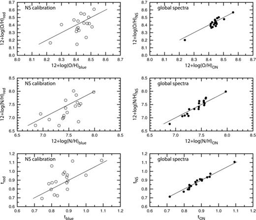
Left-hand panels: comparison among oxygen abundances (upper panel), nitrogen abundances (middle panel) and t2 electron temperatures (lower panel) in blue components and the same in the red components of the galaxies from Sample A. Right-hand panels: comparison among oxygen abundances (upper panel), nitrogen abundances (middle panel) and t2 electron temperatures (lower panel) determined from global line fluxes using the NS-calibration with the same derived using the ON-calibration. The solid lines represent equal values.
Since the SDSS spectra are closer to global spectra of galaxies rather than to spectra of individual H ii regions, the abundances determined from the SDSS spectra are ‘global abundances'. For our sample of galaxies we can determine the ‘global flux’ in every emission line as the sum of fluxes from the blue and red components, and estimate the global abundances using the NS-calibration. However, as the global flux in the [O ii]λ3727+λ3729 doublet can be measured in the spectra considered here, it is possible to estimate the global oxygen and nitrogen abundances and t2 electron temperatures using another empirical calibration, the ON-calibration (Pilyugin, Vílchez & Thuan 2010). The ON-calibration relations express the abundances (and electron temperatures) in terms of the fluxes in the strong emission lines O++, O+ and N+. It has also been derived using the spectra of H ii regions with well-measured electron temperatures as calibration data points.
The resultant global abundances and electron temperatures are given in Table 1. The right-hand panels of Fig. 10 show a comparison of global oxygen abundances (upper panel), nitrogen abundances (middle panel) and t2 electron temperatures (lower panel) in Sample A determined using the NS- and ON-calibrations. Fig. 10 also shows that the oxygen and nitrogen abundances, as well as the t2 electron temperatures, derived using the NS- and ON-calibrations, are in a good agreement, which can be considered as evidence that our abundances and temperatures are realistic.
As was noted above, the [S ii]λ6717/[S ii]λ6731 line ratio in the blue and red components shows a larger scatter than that in the global spectra (see Fig. 8), which may be caused by the uncertainties in the line decomposition. How do such uncertainties affect the derived abundances in the blue and red components? We argue that it can be estimated in the following way. It is known that the majority of extragalactic H ii regions are in the low-density regime (Zaritsky et al. 1994; Bresolin et al. 2005; Gutiérrez & Beckman 2010). The global spectra of all galaxies in our Sample A also show a low electron density having  cm−3 (Fig. 8). Then one can expect that the blue and red components also have a low electron density and, consequently, the Rs = [S ii]λ6717/[S ii]λ6731 line ratio in their spectra should be within the interval defined by the Rs values at Ne = 100 and 1 cm−3.
Let us first assume Rs at Ne = 100 cm−3 is the true value (Rstrue). Then the uncertainties in the line ratio in the blue components can be quantified by the value cb = Rsb/Rstrue. If the cb is larger/smaller than unity then the flux in the [S ii]λ6717 line is over-/underestimated by a factor of cb, 1 up to cb and/or the flux in the [S ii]λ6731 line is under-/overestimated by a factor of cb, 2 up to cb so that cb, 1/cb, 2= cb. One can estimate the corrected flux in the sulphur lines as (S2)cor= [S ii]λ6717/cb, 1+ [S ii]λ6731/cb, 2. It is evident that the error in S2 is a maximum when cb, 1= cb and cb, 2= 1 if [S ii]λ6717 > [S ii]λ6731 and when cb, 1= 1 and cb, 2= 1/cb if [S ii]λ6717 < [S ii]λ6731. We have then considered the two extreme cases. We have found two values of the corrected flux in the sulphur lines. The uncertainties in this line ratio in the red components can be quantified by the value cr= Rsr/Rstrue. The corrected flux (S2)cor in the sulphur lines can be estimated in the same way for the red components. The obtained values of cb and cr for galaxies in Sample A are all in the range of ∼0.7 to ∼1.3. As a result, the difference between the corrected flux (S2)cor and the observed flux (S2)obs in the sulphur lines does not exceed ∼15 per cent for any object. We plot the corrected flux (S2)cor against the observed one (S2)obs in the upper panel of Fig. 11 [open (red) circles].
![Upper panel: the corrected flux (S2)cor against the observed flux (S2)obs in the sulphur lines for the blue and red components in the galaxies in Sample A. The open (red) circles show the case when the corrected values have been estimated assuming the ‘true’ line ratio [S ii]λ6717/[S ii]λ6731 = 1.44 which corresponds to the electron density Ne= 100 cm−3 (see text). The filled (blue) circles show the corrected values obtained assuming the true line ratio [S ii]λ6717/[S ii]λ6731 = 1.29 which corresponds to the electron density Ne= 1 cm−3. The solid line shows the case of equal values. Lower panel: the corrected oxygen abundances (O/H)NS, cor against the observed abundances (O/H)NS, obs in the blue and red components in the galaxies in Sample A. The meanings of the symbols are the same as in the upper panel. The solid line shows the case of equal values. A colour version of this figure is available in the online version.](https://oup.silverchair-cdn.com/oup/backfile/Content_public/Journal/mnras/419/1/10.1111_j.1365-2966.2011.19714.x/1/m_mnras0419-0490-f11.jpeg?Expires=1750202396&Signature=N~M4J~hPQBf9eTLcjM-5tMUSnmrQEPtJM7YRPr8MA1mk5R3FrfFiiJj~luOzIXxQyq4GdyJI2xhykcm40Ua4MZiSyba0GjqyGG~FEdmVJc373GjddgdVsDurSImng85QweH32y3ExbDPQWaCm43VoKCAagf18U3LRnH5X-KAMlXMw8fW7wQJz7oiypcTFadhOTpKLeUs8fCnLKaaea8re2zq94w40sqExyibEb4ANgaRTG01dwvPPsPRKNOZH104LaKb3aPHzfOQHVjnlklNC19DYkVOiezLeGc-sTJiN9bdgPAFLmVNvBFfPHf5fnbkV6~D6LfnjU-zCnz9ltrCHQ__&Key-Pair-Id=APKAIE5G5CRDK6RD3PGA)
Upper panel: the corrected flux (S2)cor against the observed flux (S2)obs in the sulphur lines for the blue and red components in the galaxies in Sample A. The open (red) circles show the case when the corrected values have been estimated assuming the ‘true’ line ratio [S ii]λ6717/[S ii]λ6731 = 1.44 which corresponds to the electron density Ne= 100 cm−3 (see text). The filled (blue) circles show the corrected values obtained assuming the true line ratio [S ii]λ6717/[S ii]λ6731 = 1.29 which corresponds to the electron density Ne= 1 cm−3. The solid line shows the case of equal values. Lower panel: the corrected oxygen abundances (O/H)NS, cor against the observed abundances (O/H)NS, obs in the blue and red components in the galaxies in Sample A. The meanings of the symbols are the same as in the upper panel. The solid line shows the case of equal values. A colour version of this figure is available in the online version.
Let us now assume that the Rs at Ne = 1 cm−3 is the true Rstrue value. We plot the corrected flux (S2)cor against the observed one (S2)obs in the upper panel of Fig. 11 [filled (blue) circles]. The obtained values of cb and cr for galaxies in Sample A are again within the range of ∼0.7 to ∼1.3 and the difference between the corrected flux (S2)cor and the observed flux (S2)obs in the sulphur lines for blue and red components never exceeds ∼15 per cent.
One may consider the measured global Rsg= [S ii]λ6717/[S ii]λ6731 as being the true value instead of the Rs at Ne = 100 and at 1 cm−3. In such a case the differences between the corrected fluxes (S2)cor and flux (S2)obs in the sulphur lines in the blue and red components are usually less than ∼10 per cent.
We have found the corrected oxygen abundances (O/H)NS, cor in blue and red components through the NS-calibration using the values of corrected flux (S2)cor in the sulphur lines. The corrected oxygen abundances (O/H)NS, cor against the observed abundances (O/H)NS, obs are shown in the lower panel of Fig. 11. The lower panel of Fig. 11 shows that the difference between the corrected oxygen abundance (O/H)NS, cor and the observed abundance (O/H)NS, obs is less than 0.03 dex in all cases. This is because the coefficients of the terms with log S2 in the NS-calibration relations for oxygen abundance determinations are less than unity for all classes of H ii regions (hot, warm and cold) (Pilyugin & Mattsson 2011). Consequently, the uncertainty in S2 which is less than <15 per cent (or less than ∼0.07 dex) results in an error in log(O/H)NS, cor less than 0.03 dex. The difference between the corrected nitrogen abundance (N/H)NS, cor and the observed abundance (N/H)NS, obs is slightly larger, up to 0.07 dex. This is because the coefficients of the terms with log S2 in the NS-calibration relations for nitrogen abundance determinations are close to unity for cold and warm H ii regions (Pilyugin & Mattsson 2011). Hence, the given value of the uncertainty in S2 (up to 15 per cent or up to 0.07 dex) results in a similar error in log(N/H)NS, cor. Thus, the errors in the (O/H)NS and the (N/H)NS abundances caused by the uncertainties in the sulphur line decomposition are relatively small and do not affect the results significantly.
The O/H–N/O diagram provides an additional possibility to test the correctness of the determined oxygen and nitrogen abundances. The upper panel of Fig. 12 shows the O/H–N/O diagram for Sample A. The open circles show abundances derived using the NS-calibration for blue components; the plus signs show the same for red components. The filled grey (light-blue) circles show Te-based abundances in the calibration sample of H ii regions in nearby galaxies (the compilation of data from Pilyugin et al. 2010). Fig. 12 also shows that the abundances derived using the NS-calibration occupy the same region in the O/H–N/O diagram as the Te-based abundances of the calibration sample, which implies that our NS-calibration abundances are correct.
![The O/H–N/O diagram. Upper panel: the open circles show abundances derived using the NS-calibration for blue components of galaxies of Sample A; the plus signs show that for red components. The filled grey (light-blue) circles show Te-based abundances in the sample of best studied H ii regions in nearby galaxies (the compilation of data from Pilyugin et al. 2010). Lower panel: the same as the upper panel but for galaxies that lie in the [N ii]λ6584/Hα versus [O iii]λ5007/Hβ diagram between the separation lines after Kauffmann et al. (2003) and after Kewley et al. (2001) (see Fig. 2). A colour version of this figure is available in the online version.](https://oup.silverchair-cdn.com/oup/backfile/Content_public/Journal/mnras/419/1/10.1111_j.1365-2966.2011.19714.x/1/m_mnras0419-0490-f12.jpeg?Expires=1750202396&Signature=Lk9RlgaLmjYHSdEWL04dTDaY0RGSo~weLPhkEwALUeqk7u8BhwsQGffZXcHKaubXEznmj~DslVqcnfN6M~pwe2xtxMNYjaQbh0hKCmPwoxk1uBc7UYGf97c0U~PLA-gFQ7Kv5if-Imx-sWEV6QxPRORBah38wo4AqgmLto05ltcnPFQ5qr~fvvp9gHKMFxjYtmHL0Tm6tVR5LlJQMfYQl5UbXAuyRh4YAPinAGaFiPImINDJosWUy9m4PUBlbvb-hNEIgpI7zpmkx3Ozex2x~4713YWLbpUTinJs9JuQrCCaQdqtwXifWK0jHm0Wv18cMTfte5f~c1GyGyLnxKaD3A__&Key-Pair-Id=APKAIE5G5CRDK6RD3PGA)
The O/H–N/O diagram. Upper panel: the open circles show abundances derived using the NS-calibration for blue components of galaxies of Sample A; the plus signs show that for red components. The filled grey (light-blue) circles show Te-based abundances in the sample of best studied H ii regions in nearby galaxies (the compilation of data from Pilyugin et al. 2010). Lower panel: the same as the upper panel but for galaxies that lie in the [N ii]λ6584/Hα versus [O iii]λ5007/Hβ diagram between the separation lines after Kauffmann et al. (2003) and after Kewley et al. (2001) (see Fig. 2). A colour version of this figure is available in the online version.
The exact location of the dividing line between H ii regions and AGNs is still controversial (see, e.g. Kewley et al. 2001; Kauffmann et al. 2003; Stasińska et al. 2006). The objects that lie between the dividing lines [according to Kauffmann et al. (2003) and Kewley et al. (2001)] in the [N ii]λ6584/Hα versus [O iii]λ5007/Hβ diagram (see Fig. 2) are starburst-like objects if the dividing line of Kewley et al. (2001) is used but they are AGN-like objects (or, at least, they are not purely thermally photoionized objects) if the dividing line of Kauffmann et al. (2003) is used. Note, however, that the dividing line suggested by Stasińska et al. (2006) is very similar to that of Kauffmann et al. (2003).
The O/H–N/O diagram may also provide an indirect way to decide which curve [that according to Kauffmann et al. (2003) or that according to Kewley et al. (2001)] outlines best the area occupied by starburst-like objects in the BPT diagram. If objects that lie between these lines are starburst-like objects, the emission line fluxes in their spectra correspond to thermally photoionized objects. The NS-calibration (and other strong-line calibrations) developed for thermally photoionized nebulae will then provide reliable oxygen and nitrogen abundances for these objects, which will occupy the same region in the O/H–N/O diagram as H ii regions in nearby galaxies. If, on the other hand, the [N ii] fluxes are produced by non-thermal radiation or at least are enhanced by the contribution of non-thermal radiation, using the NS-calibration on these nebulae will result in too high nitrogen abundances. One may expect that the positions in the O/H–N/O diagram will be shifted significantly as compared to the positions of thermally photoionized H ii regions in nearby galaxies. The lower panel of Fig. 12 shows the O/H–N/O diagram for galaxies that lie between the two dividing lines in the [N ii]λ6584/Hα versus [O iii]λ5007/Hβ diagram together with the positions of thermally photoionized H ii regions in nearby galaxies. The positions of the galaxies considered here show a systematic shift towards a higher N/O ratio compared to the positions of the thermally photoionized H ii regions in nearby galaxies, which suggest that the emission lines are distorted by the contribution of non-thermal radiation, i.e. they are not purely thermal phoionization objects. If this is the case, the line according to Kauffmann et al. (2003) is to be favoured as it outlines the area occupied by certainly starburst-like objects in the BPT diagram. It has been assumed (e.g. by Juneau et al. 2011) that the line from Kewley et al. (2001) can be considered as the curve outlining the area occupied by ‘pure’ AGNs in the BPT diagram, and that objects that lie between the curves according to Kauffmann et al. (2003) and Kewley et al. (2001) are composite objects where both a starburst and an AGN make contributions. However, this interpretation is not indisputable (Cid Fernandes et al. 2010, 2011).
Comparison of oxygen abundances in the blue and red components and the global oxygen abundances tell us something about how representative/correct the abundances derived from the global spectra are. Fig. 13 shows the difference between oxygen abundances in the blue component and the global oxygen abundances versus the difference between oxygen abundances in the red component and the global oxygen abundances for galaxies in Sample A. Furthermore, Fig. 13 clearly shows that there is an anticorrelation between the two abundance differences described above. This means the global oxygen abundance obtained using the NS-calibration is typically in between the oxygen abundances of the blue and red components.
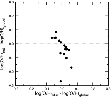
The difference between oxygen abundances in the blue component and the global oxygen abundances versus the difference between oxygen abundances in the red component and the global oxygen abundances for galaxies in Sample A.
5 CONCLUSIONS
We have extracted several hundred galaxies from the SDSS spectral data base with double-peaked emission lines in their global spectra. Among other possibilities (e.g. double-peaked AGNs), one may expect such line profiles if two strong starbursts take place simultaneously in a galaxy. We have fitted the emission lines (Hα, Hβ, [O iii]λ5007, [N ii]λ6584, [S ii]λ6717 and [S ii]λ6731) by two Gaussians in 129 spectra to separate the flux of the two (blue and red) components. A more or less reliable decomposition of the emission lines has been found for 55 spectra.
Using the standard classification [N ii]λ6584/Hα versus [O iii]λ5007/Hβ diagram and the dividing lines after Kauffmann et al. (2003), we have divided the galaxies from our sample into two subsamples: Sample A consisting of 18 galaxies where both components belong to the photoionized objects, and Sample B containing 37 galaxies that show non-thermal ionization (AGN). All the blue and red components have narrow lines regardless of their positions in the [N ii]λ6584/Hα versus [O iii]λ5007/Hβ diagram.
The differences between radial velocities of the blue and red components lie between 200 and 400 km s−1 for both subsamples. The equivalent number of ionizing stars is within the range of 104–105 O7V stars for each component in Sample A.
We have estimated the oxygen and nitrogen abundances as well as the electron temperatures for each component, and for the global spectra in Sample A, using the recent NS-calibration. We have found that the global oxygen abundance is typically in between the oxygen abundances of the blue and red components. This conclusion is based on a small sample of galaxies which, by selection, have red and blue line components of similar flux. To confirm (or reject) our conclusion a larger sample of galaxies should be considered. Applying the ON-calibration on the global spectra shows that the ON-calibration and NS-calibration give oxygen and nitrogen abundances and electron temperatures which are in a good agreement.
The O/H–N/O diagram for the galaxies in our sample gives indirect evidence suggesting that the dividing line in the [N ii]λ6584/Hα versus [O iii]λ5007/Hβ diagram from Kauffmann et al. (2003) outlines well the area occupied by starburst-like objects.
We also find that two giant H ii regions located at different positions inside the disc (one H ii region may be associated with circumnuclear star formation) seem to be responsible for the double-peaked emission lines in the spectra of Sample A. However, two starbursts in two different galaxies which are projected on top of each other, as alternative explanations of the origin of the double-peaked emission lines, cannot be excluded. Photometric and spectroscopic observations with a higher resolution may help us to resolve this issue.
Footnotes
The catalogues are available at http://www.mpa-garching.mpg.de/SDSS/
LSP and IAZ acknowledge support from the Cosmomicrophysics project of the National Academy of Sciences of Ukraine. Part of this work was supported by the Spanish Plan Nacional de Astronomía y Astrofísica under grants AYA2008-06311-C02-01, AYA2007-67965-C03-02 and AYA2010-21887-C04-01.
Funding for SDSS and SDSS-II has been provided by the Alfred P. Sloan Foundation, the Participating Institutions, the National Science Foundation, the US Department of Energy, the National Aeronautics and Space Administration, the Japanese Monbukagakusho, the Max Planck Society, and the Higher Education Funding Council for England. The SDSS web site is http://www.sdss.org/.
SDSS is managed by the Astrophysical Research Consortium for the Participating Institutions. The Participating Institutions are the American Museum of Natural History, Astrophysical Institute Potsdam, University of Basel, University of Cambridge, Case Western Reserve University, University of Chicago, Drexel University, Fermilab, the Institute for Advanced Study, the Japan Participation Group, Johns Hopkins University, the Joint Institute for Nuclear Astrophysics, the Kavli Institute for Particle Astrophysics and Cosmology, the Korean Scientist Group, the Chinese Academy of Sciences (LAMOST), Los Alamos National Laboratory, the Max-Planck-Institute for Astronomy (MPIA), the Max-Planck-Institute for Astrophysics (MPA), New Mexico State University, Ohio State University, University of Pittsburgh, University of Portsmouth, Princeton University, the United States Naval Observatory, and the University of Washington.
REFERENCES
