


Abstract
In this paper, a new method is proposed to estimate the broad-line region sizes of ultraviolet (UV) lines RuvBLR. It is applied to 3C 273. First, we derive the time lags of radio emission relative to broad emission lines Lyα and C iv by the z-transformed discrete correlation function (ZDCF) method. The broad lines lag the 5-, 8-, 15-, 22- and 37-GHz emission. The measured lags τuvob are of the order of years. For a given line, τuvob decreases as the radio frequency increases. This trend results from the radiative cooling of relativistic electrons. Both UV lines have a lag of τuvob=−2.74+0.06− 0.25 yr relative to the 37-GHz emission. These results are consistent with those derived from the Balmer lines in Paper I. Secondly, we derive the time lags of the lines Lyα, C iv, Hγ, Hβ and Hα relative to the 37-GHz emission by the flux randomization/random subset selection (FR/RSS) Monte Carlo method. The measured lags are τob=−3.40+0.31− 0.05, −3.40+0.41− 0.14, −2.06+0.36− 0.92, −3.40+1.15− 0.20 and −3.56+0.35− 0.18 yr for the lines Lyα, C iv, Hγ, Hβ and Hα, respectively. These estimated lags are consistent with those derived by the ZDCF method within the uncertainties. Based on the new method, we derive RuvBLR= 2.54+0.71− 0.35 to 4.01+0.90− 1.16 and 2.54+0.80− 0.43 to 4.01+0.98− 1.24 light-years for the Lyα and C iv lines, respectively. Considering the uncertainties, these estimated sizes are consistent with those obtained in the classical reverberation mapping for the UV and the Balmer lines. This indicates that their emitting regions are not separated so large as in the classical mapping of the UV and optical lines. These results seem to depart from the stratified ionization structures obtained in the classical mapping.
1 INTRODUCTION
Based on the photoionization assumption and the time lags between both variations of broad emission lines and continuum, reverberation mapping observations are able to determine the sizes of broad-line regions (BLR) for type 1 active galactic nuclei (AGNs; see e.g. Peterson 1993; Kaspi & Netzer 1999; Wandel, Peterson & Malkan 1999; Kaspi et al. 2000, 2005, 2007; Peterson et al. 2000, 2004, 2005; Vestergaard & Peterson 2006). The classical reverberation mapping is very successful in estimates of the BLR sizes. In these reverberation mapping observations, the stratified ionization structures of the BLRs are found for various types of broad emission lines, such as the Balmer lines and the He ii and He i lines seen in NGC 5548 (e.g. Clavel et al. 1991) and Mrk 110 (Kollatschny et al. 2001; Kollatschny 2003), and the Balmer lines and the Lyα and C iv lines seen in 3C 273 (Paltani & Türler 2005). The higher ionized lines respond systematically faster to the continuum variations. The separation of emission regions for these lines spans a large range. The higher ionized lines are emitted at the smaller distances from the ionizing continuum source.
The photoionization assumption requires that the frequency of ionizing continuum must not be lower than those of the emission lines produced through the photoionization process (e.g. Peterson 1993). The ultraviolet (UV) and optical continua are used as the ionizing continuum in these reverberation mapping observations. This treatment leads to underestimation of the BLR sizes RBLR, as seen in e.g. 3C 273 (Paltani & Türler 2005). For the Balmer lines of 3C 273, the BLR sizes derived from the UV continuum around 1300 Å are between two and four times larger than those from the optical continuum around 5000 Å. Furthermore, their estimates are in excellent agreement with each other (Paltani & Türler 2005), while in Kaspi et al. (2000) the Hα lag is 60 per cent larger than that of Hγ. It seems to be appropriate to regard the UV continuum as the ionizing continuum of the Balmer lines. For the UV lines Lyα and C iv, it should be appropriate to regard the extreme ultraviolet (EUV) and soft X-ray continua as the ionizing continuum. Wandel et al. (1999) regarded the EUV photons as the ionizing source of Hβ. Wandel (1997) showed that the soft X-rays are better to represent the ionizing flux. The photons above 912 Å are believed to be the main sources of line formation via photoionization, and they should be related to the emission lines seen in the near-ultraviolet (NUV) and optical regimes (Telfer et al. 2002). Thus it seems to be inapposite of using the UV continuum as the ionizing continuum of the UV lines to estimate the BLR sizes.
Disturbances in the central engine are likely transported outward along the relativistic jets. This was supported by observations that dips in the X-ray emission are followed by ejections of bright superluminal knots in the radio jets of AGNs (Marscher et al. 2002; Chaterjee et al. 2009; Arshakian et al. 2010). The events in the central engine will have a direct effect on the events in the radio jets (e.g. Marscher et al. 2002; Chaterjee et al. 2009). According to the reverberation mapping model (e.g. Blandford & McMee 1982), the events in the central engine also have a direct effect on the events in the BLR through the photoionization process. Thus it is expected that there should exist correlations between both variations of the broad emission lines from the BLR and the radio emission from the relativistic jet aligned with the line of sight. Especially, the correlations have time lags of the broad lines relative to the radio emission and the time lags are related to the position of radio-emitting region Rradio (Liu, Bai & Wang 2011, hereafter Paper I). Both optical and UV lines should give the same Rradio from their time lags relative to the radio emission. In this paper, we give a method to estimate the BLR sizes of the UV lines from the BLR sizes of the optical lines and their time lags relative to the radio emission.
2 METHOD
For the UV and optical broad emission lines, one can estimate the time lags of lines by using the radio emission as the common reference. As τuvob and τoptob are measured, one can estimate RuvBLR from RoptBLR, which is obtained in the reverberation mapping for the optical lines with an appropriate ionizing continuum. This new method can improve the classical reverberation mapping, especially on blazars that have strongly beamed emission at optical, UV and X-ray bands and also have strong radio emission.
3 APPLICATION TO 3C 273
The flat spectrum radio quasar 3C 273 was first identified as a quasar at redshift z = 0.158 by Schmidt (1963). It is one of the best studied AGNs in all bands (e.g. von Montigny et al. 1997; Türler et al. 1999; Soldi et al. 2008). It is also one of the bright extragalactic objects in the γ-ray sky. Its jet is one-sided, with no signs of emission from the counterjet side (Unwin et al. 1985). The blue-bump observed in 3C 273 is attributed to thermal continuum emission from the inner accretion disc (Shields 1978). Fe Kα lines observed in 3C 273 are shown to be from an accretion disc around a supermassive black hole (Yaqoob & Serlemitsos 2000; Torres et al. 2003). The supermassive black hole accreting material to form accretion disc powers the central engine in this object.
3.1 Data and analysis of time lags
This paper makes use of data from the 3C 273 data base hosted by the ISDC1 (Türler et al. 1999). We consider the radio light curves used in Paper I. Light curves of broad UV lines Lyα and C iv are taken from Paltani & Türler (2003). The sampling rates of the Lyα and C iv lines are around six times per year, which are comparable with those of the Balmer lines used in Paper I. First, we employ the same analysis method for the UV lines as the Balmer lines Hα, Hβ and Hγ used in Paper I.
As in Paper I, the z-transformed discrete correlation function (ZDCF; Alexander 1997) is used to analyse the time lags that are preferred to be characterized by the centroid τcent of the ZDCF. The centroid time lag τcent is computed by using all the points with correlation coefficients r≥ 0.8rmax, where rmax is the maximum of correlation coefficients in the ZDCF bumps closer to the zero-lag. The calculated ZDCFs between the radio and broad-line light curves are presented in Fig. 1. The horizontal and vertical error bars in Fig. 1 represent the 68.3 per cent confidence intervals in the time lags and the relevant correlation coefficients, respectively. The ZDCFs in Fig. 1 have a common significant feature, i.e. the negative lag closer to the zero-lag. All the ZDCF bumps closer to the zero-lag have a good profile. The measured time lags are listed in Table 1. The centroid τcent is calculated by τcent=∑τ(i)r(i)/∑r(i), where τ(i) and r(i) are the values of the ith data pair with r≥ 0.8rmax. The errors of τcent are calculated by Δτ±cent={∑[Δτ±(i)r(i) +τ(i)Δr±(i)]∑r(i) −∑τ(i)r(i)∑Δr±(i)}/[∑r(i)]2, where Δτ±(i) and Δr±(i) are the relevant errors of τ(i) and r(i), respectively.
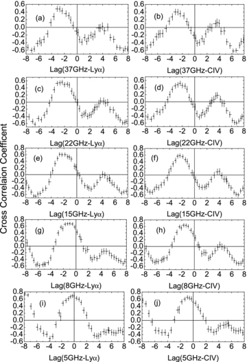
ZDCFs between Lyα and 37 GHz (a), 22 GHz (c), 15 GHz (e), 8 GHz (g) and 5 GHz (i); ZDCFs between C iv and 37 GHz (b), 22 GHz (d), 15 GHz (f), 8 GHz (h) and 5 GHz (j). The x-axis is in units of yr.
Time lags between emission lines and radio emission. The sign of time lag is defined as τcent=tradio−tline. Time lags are in units of yr.
| Lines | 5 GHz | 8 GHz | 15 GHz | 22 GHz | 37 GHz |
| C iv | −0.93+0.06−0.21 | −1.67+0.04−0.18 | −2.29+0.05−0.22 | −2.34+0.05−0.23 | −2.74+0.06−0.25 |
| Lyα | −0.24+0.05−0.20 | −1.16+0.05−0.22 | −2.08+0.04−0.20 | −2.17+0.06−0.23 | −2.74+0.06−0.25 |
| Lines | 5 GHz | 8 GHz | 15 GHz | 22 GHz | 37 GHz |
| C iv | −0.93+0.06−0.21 | −1.67+0.04−0.18 | −2.29+0.05−0.22 | −2.34+0.05−0.23 | −2.74+0.06−0.25 |
| Lyα | −0.24+0.05−0.20 | −1.16+0.05−0.22 | −2.08+0.04−0.20 | −2.17+0.06−0.23 | −2.74+0.06−0.25 |
Our results show that the UV line variations lag the radio variations of 5, 8, 15, 22 and 37 GHz (see Fig. 1). The measured time lags are of the order of years (see Table 1). For a given line, the relevant time lags generally decrease as radio frequency increases from 5 to 37 GHz. This trend most likely results from the radiative cooling of relativistic electrons (see Paper I). These results are consistent with those obtained in Paper I. Hereafter, τcent is equivalent to τob.
The uncertainties of each point in the ZDCFs only take into account the uncertainties from the measurements by Monte Carlo simulation. Thus the uncertainties in the cross-correlation results will be estimated by using the model-independent FR/RSS Monte Carlo method described by Peterson et al. (1998). The quantities we are concerned with are related to the time lags of Lyα, C iv, Hα, Hβ and Hγ relative to the 37-GHz emission. Thus we only recompute the uncertainties of time lags for these five lines relative to the 37-GHz emission. The median of distribution of the time lags estimated by Monte Carlo simulations of 1000 runs is taken to be the time lag of line relative to the 37-GHz emission. The confidence intervals are estimated on the basis of the distribution of the time lags simulated. The calculated results are listed in Table 2. The time lags are presented with centroid and peak values. For these five lines, their time lags are well consistent with each other within ±1σ. These time lags of Hα, Hβ and Hγ listed in Table 2 are well consistent with those listed in table 1 of Paper I. The good agreements between these time lags estimated by the FR/RSS method and the ZDCF method confirm the reliability of the results of Paper I. Here, the uncertainties of time lags are larger than those estimated in the ZDCF method. This indicates underestimation of the uncertainties in the ZDCF method. Thus the uncertainties presented in Table 2 will be used in the relevant calculations of uncertainties.
Time lags between emission lines and 37-GHz emission. The sign of time lag is defined as τ=tradio−tline. Time lags are in units of yr. The numbers in brackets give the ±1σ, ±2σ and ±3σ confidence intervals.
| Lines | τcent | τpeak |
| Lyα | −3.40 {+0.31−0.05 {+0.68−0.19 {+1.12−1.00 | −3.40 {+0.10−0.10 {+0.90−0.10 {+2.00−1.10 |
| C iv | −3.40 {+0.41−0.14 {+0.95−0.51 {+1.42−1.05 | −3.40 {+0.20−0.10 {+1.00−1.00 {+1.90−1.10 |
| Hγ | −2.06 {+0.36−0.92 {+0.51−1.54 {+0.56−2.68 | −1.90 {+0.30−1.50 {+0.40−1.80 {+0.40−3.40 |
| Hβ | −3.40 {+1.15−0.20 {+1.90−0.44 {+2.06−0.90 | −3.40 {+1.80−0.30 {+1.90−0.50 {+2.00−1.10 |
| Hα | −3.56 {+0.35−0.18 {+0.86−0.95 {+0.96−1.14 | −3.60 {+0.20−0.10 {+1.00−1.00 {+1.00−1.60 |
3.2 Estimation of BLR sizes
Both UV lines, Lyα and C iv, have a time lag of τuvob=−2.74 yr relative to the 37-GHz emission (see Table 1). Based on the typical size of optical lines Hα, Hβ and Hγ, RoptBLR = 2.70 light-years (ly) (Paltani & Türler 2005), τoptob=−2.86 yr obtained in Paper I for the Balmer lines, τuvob=−2.74 yr and z = 0.158, we obtain RuvBLR = 2.60 ly from equation (2). Without considering the uncertainties, RuvBLR = 2.60 ly seems to be larger than those values of 1.2–1.9 ly obtained in the reverberation mapping (Paltani & Türler 2005). Furthermore, the lines Lyα and C iv have the same time lag of τuvob=−2.74 yr relative to the 37-GHz emission. These BLR sizes estimated by equation (2) for the lines Lyα and C iv are in excellent agreement with each other. These above results are based on the ZDCF method.
From equation (2), we have the uncertainty transfer expression ΔRuvBLR=ΔRoptBLR+ (Δτoptob+Δτuvob)c/(1 +z), which is the maximum uncertainty transfer expression and will maximize |ΔRuvBLR| due to possible combinations of ΔRoptBLR, Δτoptob and Δτuvob. Based on τcent listed in Table 2, equation (2) and RoptBLR of Paltani & Türler (2005), we estimate RuvBLR for the lines Lyα and C iv in virtue of the lines Hα, Hβ and Hγ. The transferred uncertainties are estimated by the uncertainty transfer expression with the ±1σ, ±2σ and ±3σ confidence intervals of τcent and RoptBLR. The estimated results are presented in Table 3. These estimated RuvBLR are consistent with each other within ±1σ. There seems to be a ‘flaw’ in the 3σ uncertainties of RuvBLR in the cases of the lines Hβ and Hγ, due to which the 3σ uncertainty causes RuvBLR to be negative (see Table 3). In fact, this ‘flaw’ just means that within 3σ uncertainty, RuvBLR is consistent with zero. These above results are based on the model-independent FR/RSS Monte Carlo method (Peterson et al. 1998), which contains the DCF method (Edelson & Krolik 1988).
RuvBLR estimated for the Lyα and C iv lines in the cases of the Hα, Hβ and Hγ lines. RuvBLR is in units of ly. The numbers in brackets give the transferred uncertainties from the ±1σ, ±2σ and ±3σ confidence intervals of RoptBLR, τoptob and τuvob.
| Lines | Hα | Hβ | Hγ |
| Lyα | 2.54 {+0.71−0.35 {+1.66−1.34 {+2.38−2.41 | 2.58 {+1.45−0.41 {+2.64−0.87 {+3.46−2.84 | 4.01 {+0.90−1.16 {+1.74−2.18 {+2.45−5.81 |
| C iv | 2.54 {+0.80−0.43 {+1.89−1.62 {+2.64−2.45 | 2.58 {+1.54−0.48 {+2.87−1.15 {+3.72−2.88 | 4.01 {+0.98−1.24 {+1.97−2.46 {+2.71−5.85 |
| Lines | Hα | Hβ | Hγ |
| Lyα | 2.54 {+0.71−0.35 {+1.66−1.34 {+2.38−2.41 | 2.58 {+1.45−0.41 {+2.64−0.87 {+3.46−2.84 | 4.01 {+0.90−1.16 {+1.74−2.18 {+2.45−5.81 |
| C iv | 2.54 {+0.80−0.43 {+1.89−1.62 {+2.64−2.45 | 2.58 {+1.54−0.48 {+2.87−1.15 {+3.72−2.88 | 4.01 {+0.98−1.24 {+1.97−2.46 {+2.71−5.85 |
These RuvBLR estimated from the ZDCF method are consistent with those from the FR/RSS method within the uncertainties. The BLR sizes of the lines Lyα and C iv derived from the classical mapping are consistent with those presented in Table 3 within about ±2σ (see table 1 of Paltani & Türler 2005). These agreements indicate for both UV lines that these estimated RuvBLR are reliable and reasonable. Our results indicate that the separation between the BLRs of the lines Lyα and C iv are not so large as in the classical mapping (see table 1 of Paltani & Türler 2005). Our results also indicate for 3C 273 that the BLRs of UV lines are blended with or very close to those of optical lines (see table 4 of Paltani & Türler 2005).
4 DISCUSSION
The soft X-rays and the EUV continuum might be suitable to be used as the ionizing continuum for the Lyα and C iv lines. The soft X-rays are better to represent the ionizing flux (Laor 1990; Wandel 1997; Fiore et al. 1998). Wandel et al. (1999) regarded the EUV photons as the ionizing source of Hβ. The photons above 912 Å are believed to be the main sources of line formation via photoionization and should be related to the emission lines seen in the NUV and optical regimes (Telfer et al. 2002). However, the soft X-ray data are not available for many AGNs (e.g. Wandel et al. 1999). For blazars, the central ionizing continua will be strongly contaminated by the beamed emission from the relativistic jets, so that the blue-bump is not observable for most of blazars. Paltani, Courvoisier & Walter (1998) showed for 3C 273 that the optical continuum is strongly contaminated by the beamed emission from the relativistic jet and it appears unsuitable for studying the time lags between the ionizing continuum and the lines. Paltani & Türler (2005) argued that the UV continuum is much closer to the ionizing continuum than the optical continuum used by Kaspi et al. (2000). They used the 1300-Å continuum to infer the time lags of the Balmer lines and found better estimate for the optical BLR than Kaspi et al. (2000). The underlying physical condition in the photoionization model is that the frequencies of ionizing photons must not be lower than those of the emission lines generated via the photoionization process. Thus it is appropriate to regard the 1300-Å continuum as the ionizing continuum of the Hα, Hβ and Hγ lines because its frequency is higher than those of the lines. However, it should not be appropriate to regard the 1300-Å continuum as the ionizing continuum of the Lyα line because its frequency is less than that of the line.
There are several fundamental assumptions made in the reverberation mapping, and one of them is that there is a simple, although not necessarily linear, relationship between the observable continuum and the ionizing continuum that is driving the lines (Peterson 1993). The assumption cannot be tested directly. The close correspondence between continuum and line light curves gives us some confidence that this assumption is valid at some level of approximation (Peterson 1993). However, observations indicate a complicated relationship between variations of optical/UV and EUV/X-ray bands, e.g. Seyfert type 1 AGN NGC 4051 (Shemmer et al. 2003; Arévalo et al. 2008). The complex X-ray, EUV, UV and optical correlations are explained as a possible combination of X-ray reprocessing, thermal Compton upscattering of optical/UV seed photons and disturbances propagating from outer (optically emitting) parts of accretion disc into its inner (X-ray emitting) region (Shemmer et al. 2003; Arévalo et al. 2008). The complex relationships between these bands indicate that it is difficult to choose the ionizing continuum and its appropriate agency. This new method we proposed to estimate the BLR size of the UV lines could avoid the choice of the ionizing continuum and its agency.
The complex relationships between the UV, EUV and X-ray continuum light curves may depend on the origin of energies emitted at these bands. If the UV continuum is produced via thermal reprocessing of the X-rays, the X-rays will lead the UV photons. If the UV, EUV and X-rays are generated via viscous dissipation in accretion disc, the UV will lead the EUV and X-rays. The EUV and X-ray emission might be from the same origin. Observations of NGC 5548 for around 10 days show no time lag of X-rays from EUV flux on time-scales longer than a day (Haba et al. 2003). If the X-rays are produced by the upscattering of UV seed photons, e.g. the X-rays are generated in hotter corona and the UV seed photons are from disc, then the UV variations will lead the X-rays. The lag of the X-rays relative to the UV variations corresponds to the light travel time between the seed photon source and a Compton upscattering region. This case seems to be supported by observations of NGC 3516 that the optical variations lead the X-rays by ∼100 days (Maoz, Edelson & Nandra 2000). Their monitoring lasted for ∼550 days. They showed that the correlation signal at 100 days is entirely due to the slow (variability time-scale ≳30 d) components of the light curves. During the whole monitoring period, the more rapidly changing components of the light curves are uncorrelated at any lag. The light-travel distance of this lag of X-rays relative to optical variations is much larger than the BLR size of ∼11 light-days (Wanders et al. 1999). These outbursts, which dominate this lag of ∼100 days, in the optical and X-ray light curves have a variability time-scale of the order of ∼100 days. Observations of NGC 5548 for ∼10 days show that the time lag between the EUV and X-ray flux is negligible relative to the light travel time of the BLR size (see Haba et al. 2003). Observations of NGC 3783 spanning 2 yr show that the optical light curves lag the X-rays by 3–9 d (Arévalo et al. 2009). This delay points at optical variability produced by X-ray reprocessing. This time lag is comparable to that of optical lines relative to the continuum, ∼8 d (Reichert et al. 1994; Stirpe et al. 1994). The large time lags between these continuum bands should exist in the long-term correlations, e.g. NGC 3516. The small lags should exist in the short-term correlations, e.g. NGC 4151 and 7469 (Edelson et al. 1996; Nandra et al. 1998). The light curves used to estimate the lags for NGC 4151 and 7469 span time intervals  30 d. It is possible that the light curves used to measure the lags do not have enough time-spans, so that the large lags cannot be measured even if they indeed exist. These observational facts indicate complex relationships between these continuum bands and between the time lags within these bands and the BLR sizes. Thus the choice of ionizing continuum would significantly influence the time lags of emission lines relative to the observable continua, e.g. 3C 273 (see Paltani & Türler 2005).
According to the results of this paper, if the UV BLR size is taken to be 2.6 ly for 3C 273, which means that if we had known the light curve of the ionizing continuum (say the X-ray light curve), the time lag would have been 2.6 yr. On the other hand, the UV lines are lagging the UV continuum by about 1.5 yr (Paltani & Türler 2005). This means that the UV continuum light curve must lag the X-ray light curve by about 1.1 yr, which means that the UV-emitting place is far from the X-ray emitting place by 1.1 ly. The UV continuum light curve has a characteristic variability time-scale ∼2.0 yr, which is estimated from the zero-crossing time of the autocorrelation function (ACF) of its light curve. The zero-crossing time of the ACF of light curve is a well-defined quantity and is used as a characteristic variability time-scale (e.g. Netzer et al. 1996; Alexander 1997; Giveon et al. 1999). There is a simple relation between the ACF and the first-order structure function that is used in variability studies to estimate the variability time-scale (Giveon et al. 1999). If this characteristic time-scale ∼2.0 yr corresponds to the size of the UV-emitting region in accretion disc, the UV-emitting position will be ∼1.0 ly far from the place that emits the X-rays. This distance of ∼1.0 ly is consistent with that value of ∼1.1 ly deduced above. Thus it is a reasonable size for the accretion disc, wherein the place that emits the UV continuum is far from the place that emits the X-rays by 1.1 ly.
For the Balmer lines Hα, Hβ and Hγ of 3C 273, the BLR sizes derived from the 1300-Å continuum are between two and four times larger than those from the optical continuum around 5000 Å (Paltani & Türler 2005). Furthermore, their estimates are in excellent agreement with each other, while in Kaspi et al. (2000) the Hα lag is 60 per cent larger than the Hγ lag. Thus the lines Lyα and C iv should have larger BLR sizes as the soft X-rays rather than the 1300-Å continuum are taken to be the ionizing continuum. However, the soft X-rays do not have enough data for 3C 273 (Paltani & Türler 2003). Our new method resolves the problem to choose the ionizing continuum. Based on equation (2), RoptBLR = 2.70 ly, τoptob=−2.86 yr, τuvob=−2.74 yr and z = 0.158, we obtain RuvBLR = 2.60 ly for the lines Lyα and C iv. If the time lags of the lines derived by the FR/RSS method are used to estimate the UV BLR sizes by virtue of the Balmer lines, then RuvBLR = 2.54–4.01 ly. These estimated sizes are consistent with each other within ±1σ. The BLR sizes of the lines Lyα and C iv obtained in the classical mapping are consistent with these estimated sizes within about ±2σ (see Table 3 of this paper and table 1 of Paltani & Türler 2005). Considering the uncertainties, the BLR sizes of the lines Hα, Hβ and Hγ are well consistent with these estimated sizes of the lines Lyα and C iv (see table 4 of Paltani & Türler 2005). These results indicate that the BLRs of UV lines are blended with or very close to those of optical lines. Our results seem to depart from the stratified ionization structures obtained in the classical mapping.
The new method proposed in this paper is based on the method proposed in Paper I. The key of the two methods requires that the central disturbance signals are transported to the BLR and the jets. This key requirement of the two methods is supported by observational research (Marscher et al. 2002; Chaterjee et al. 2009; Arshakian et al. 2010) and theoretical research (e.g. Blandford & McMee 1982; Meier, Koide & Uchida 2001; Koide et al. 2002). The central disturbance signals transported to the BLR and the jets are likely the physical link between both variations of the emission lines from the BLR and the beamed emission from the relativistic jet aligned with the line of sight.
In Paper I, we found for the broad Balmer lines that the lags for a given line generally decrease as radio frequency increases and that this trend results from the radiative cooling of relativistic electrons. For the UV lines Lyα and C iv, there is the same trend as for the Balmer lines (see Table 1). The measured lags τoblag between the 5-, 8-, 15-, 22- and 37-GHz emission were compared with the differences of Δτcent between τcent for the Balmer lines (see fig. 7 in Paper I). In this paper, we compare τoblag with Δτcent for the UV lines in Fig. 2. The line of Δτcent=τoblag is consistent with the measured data points for both the Balmer lines and the UV lines (see Fig. 2). This agreement further confirms that the trend, i.e. the lags for a given line generally decrease as radio frequency increases, results from the radiative cooling of relativistic electrons.
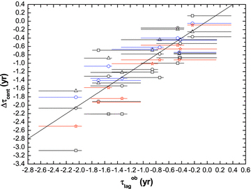
Δτcent between τcent for the five emission lines versus τoblag. Circles denote Hα, squares denote Hβ, triangles denote Hγ, blue hexagons denote C iv and red pentacles denote Lyα. Solid line is for Δτcent=τoblag.
The broad-line light curves do not experience relativistic shortening of variation time-scales. The light curves generated by a relativistic jet closely aligned to the line of sight experience the relativistic shortening of variation time-scales. The relativistic effects would not have significant influence on the estimates of time lags between the broad lines and the radio emission (see Paper I). For testing the correctness of the time lags measured by these ZDCFs, we compare the 37-GHz light curve with the broad-line light curves moved horizontally and vertically (see Fig. 3). For the negative lags used (see Fig. 1), the line light curves are moved left by 2.7 yr. These moved line light curves basically follow the variation trend of the radio light curve (see Fig. 3). This indicates that the measured lags of τuvob=−2.74 yr are reliable and reasonable. For the optical lines Hα, Hβ and Hγ, there are the negative lags and the positive lags relative to the 37-GHz emission (see Paper I). The lags should be positive or negative; however, the current data do not allow us to discriminate between the two cases for the Balmer lines. On the contrary, there are only the negative lags for the Lyα and C iv lines relative to the 37-GHz emission because these UV light curves span much longer time intervals than these optical line light curves do. The longer interval light curves do indeed resolve the problem of the negative or positive lags emerging in Paper I, due to the shortage of interval spans of these optical line light curves.
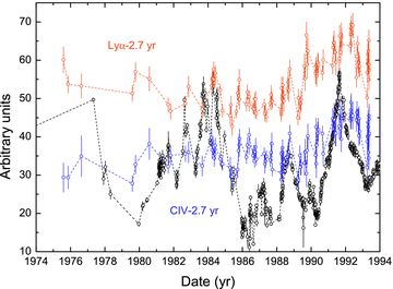
Comparison of the 37-GHz light curve with the Lyα and C iv line light curves moved along the x- and y-axes.
5 CONCLUSIONS
In this paper, we propose a new method to estimate the BLR sizes of the UV lines, RuvBLR. It is applied to 3C 273. We derive the time lags of the radio emission relative to the broad emission lines Lyα and C iv. These broad lines lag the 5-, 8-, 15-, 22- and 37-GHz emission. The measured lags τuvob are of the order of years. For a given line, τuvob generally decreases as radio frequency increases. This trend results from the radiative cooling of relativistic electrons. Both the Lyα and C iv lines have a time lag of τuvob=−2.74 yr relative to the 37-GHz emission. These results are consistent with those derived from the Balmer lines in Paper I. Based on τuvob=−2.74 yr, τoptob=−2.86 yr, RoptBLR = 2.70 ly and z = 0.158, we obtain RuvBLR = 2.60 ly from equation (2). The time lags estimated by the FR/RSS method are τuvob=−3.40+0.31− 0.05 and −3.40+0.41− 0.14 yr for the lines Lyα and C iv, respectively. These estimated lags are consistent with those lags estimated by the ZDCF method. The time lags estimated by the FR/RSS method are τoptob=−3.56+0.35− 0.18, −3.40+1.15− 0.20 and −2.06+0.36− 0.92 yr for the lines Hα, Hβ and Hγ, respectively, relative to the 37-GHz emission. These estimated lags are well consistent with those lags estimated by the ZDCF method in Paper I. These lags estimated by the FR/RSS method for the UV lines and the Balmer lines are well consistent with each other within the uncertainties. Based on these estimated lags, RoptBLR obtained in the classical mapping and equation (2), we derive the BLR sizes of the UV lines. These estimated sizes of Lyα are RuvBLR = 2.54+0.71− 0.35, 2.58+1.45− 0.41 and 4.01+0.90− 1.16 ly in the cases of Hα, Hβ and Hγ, respectively. These estimated sizes of C iv are RuvBLR = 2.54+0.80− 0.43, 2.58+1.54− 0.48 and 4.01+0.98− 1.24 ly in the cases of Hα, Hβ and Hγ, respectively. These estimated sizes are well consistent with each other within ±1σ. These estimated sizes of the UV lines are consistent with those UV BLR sizes obtained in the classical mapping within about ±2σ (see Table 3 of this paper and table 1 of Paltani & Türler 2005). Considering the uncertainties, these estimated sizes of the UV lines are well consistent with the BLR sizes of the Balmer lines obtained in the classical mapping (see table 4 of Paltani & Türler 2005). These results indicate that the BLRs of UV lines are blended with or very close to those of the optical lines. Our results seem to depart from the stratified ionization structures obtained in the classical mapping.
We are grateful to the anonymous referee for constructive comments and suggestions leading to significant improvement of this paper. HTL and SKL thank the West PhD project of the Training Programme for the Talents of West Light Foundation of the CAS and the National Natural Science Foundation of China (NSFC; Grant 10903025) for financial support. JMB acknowledges the support of the NSFC (Grants 10973034 and 10778702). JMW is supported by the NSFC (Grant 10733010). JMB and JMW acknowledge the support of the 973 Programme (Grant 2009CB824800).
REFERENCES
