Angular correlation function of 1.5 million luminous red galaxies: clustering evolution and a search for baryon acoustic oscillations Free

Abstract

1 INTRODUCTION

The galaxy two-point function whether in its correlation function or power spectrum form has long been recognized as a powerful statistical tool for studying large-scale structure (LSS) of the Universe (Peebles 1980). In an isotropic and homogeneous Universe, if the density fluctuation arises from a Gaussian random process, the two-point correlation function, ξ(r), and its Fourier transform, P(k), contain a complete description of such fluctuations. It has been used to measure the clustering strength of galaxies in numerous galaxy surveys (see e.g. Groth & Peebles 1977; Shanks et al. 1989; Baugh & Efstathiou 1993; Ratcliffe et al. 1998) and the observed ξ(r) is reasonably well represented by a power law of the form ξ(r) = (r/r₀)^−1.8 over a large range of scales, ≈100 h⁻¹ kpc–10 h⁻¹ Mpc, where r₀ is approximately 5 h⁻¹ Mpc.

More recently, large galaxy redshift surveys have become available [Sloan Digital Sky Survey (SDSS): York et al. 2000, Two-degree-Field Galaxy Redshift Survey (2dFGRS): Colless et al. 2001] and these surveys provide a perfect opportunity to exploit the two-point function as a tool to constrain cosmological parameters (Hawkins et al. 2003; Cole et al. 2005; Eisenstein et al. 2005; Tegmark et al. 2006; Percival et al. 2007) which in turn provides an excellent test for our current understanding of the Universe and the processes by which the LSS were formed.

In the past, when galaxy redshift surveys were less available, the angular correlation function, w(θ), was heavily utilized in the analysis of imaging galaxy samples. The spatial correlation function, ξ(r), can be related to w(θ) via Limber’s equation (Limber 1953), alternatively w(θ) can be inverted to ξ(r) using Lucy’s iterative technique (Lucy 1974), both approaches providing a means to recover the 3D clustering information numerically. Even today, galaxy imaging surveys still tend to cover a bigger area of the sky and occupy a larger volume than redshift surveys and therefore could offer a route to a more accurate estimation of the correlation function and power spectrum (see e.g. Baugh & Efstathiou 1993). One of the disadvantages of using w(θ) is the dilution of the clustering signal from projection and hence any small-scale/sharp feature which might exist in the 3D clustering may not be observable in w(θ).

As mentioned above, the correlation function at small to intermediate scales can be approximately described by a single power law which also results in a power-law w(θ) but with a slope of 1 −γ. However with larger sample sizes, recent analyses of galaxy distributions start to show a deviation from a simple power law (Zehavi et al. 2005b; Phleps et al. 2006; Ross et al. 2007; Blake, Collister & Lahav 2008, see also Shanks et al. 1983). This poses a challenge for a physical explanation and understanding of non-linear evolution of structure formation. Several authors attempted to fit such correlation function using a description of halo model framework (e.g. Cooray & Sheth 2002) invoking a transition between one- and two-halo terms which occurs at ≈1 h⁻¹ Mpc where the feature is observed. This distance scale could potentially be used as a ‘standard ruler’ in tracking the expansion history of the Universe, provided that its physical origin is well understood and the scale can be accurately calibrated.

Another feature in the correlation function predicted by the standard Λcold dark matter (ΛCDM) model is the ‘baryon acoustic oscillations’ (BAO). BAO arise from sound waves that propagated in the hot plasma of tightly coupled photons and baryons in the early Universe. As the Universe expands and temperature drops below 3000 K, and photons decouple from the baryons at the so-called ‘epoch of recombination’. The sound speed drops dramatically and oscillatory pattern imprinted on the baryon distribution as well as the temperature distribution of the photons which approximately 13 billions years after the big bang revealed as the acoustic oscillations in the temperature anisotropies of the cosmic microwave background. The equivalent but attenuated feature exists in the clustering of matter, as baryons fall into dark matter potential wells after the recombination. In recent years, the acoustic peak scale in the LSS has been proposed as a potential ‘standard ruler’ (e.g. Blake & Glazebrook 2003; Glazebrook et al. 2007; McDonald & Eisenstein 2007) for constraining the dark energy equation of state (w=p/ρc²) and its evolution.

For the BAO approach to the study of dark energy to yield a competitive result, a large survey of several million galaxies is generally required (Blake & Glazebrook 2003; Seo & Eisenstein 2003; Parkinson et al. 2007; Angulo et al. 2008). A galaxy spectroscopic redshift survey would require a substantial amount of time and resources. An alternative route which will enable a quicker and larger area covered is through the use of photometric redshift (hereafter photo-z) at the expense of the ability to probe the radial component directly. The photo-z errors are usually worse than spectroscopic redshift errors, but this can be compensated by a larger survey and deeper imaging.

The potential of the distribution of luminous red galaxies (LRGs) as a powerful cosmological probe has long been appreciated (Gladders & Yee 2000; Eisenstein et al. 2001, hereafter E01). Their intrinsically high luminosities provide us with at least two advantages, one being the ability to observe such a population out to a greater distance whilst the other is the possibility of detecting the small overdensity of the BAO in matter distribution at ≈100 h⁻¹ Mpc owing to their high linear bias.1 In addition, their typically uniform spectral energy distributions (SEDs) allow a homogeneous sample to be selected over the volume of interest. Moreover, the strong 4000 Å break in their SEDs makes them an ideal candidate for the photometric redshift route or even a colour–magnitude cut as demonstrated by the success of the target selection algorithm of three LRG spectroscopic follow-ups using SDSS imaging. In fact, the first clear detection of the BAO in the galaxy distribution came from the analysis of LRG clustering at low redshift (Eisenstein et al. 2005).

Here, we shall present new measurements of the angular correlation functions determined from colour-selected LRG samples. We shall show that this route provides redshift distribution, n(z), widths that are close to the current photo-z accuracy, with none of the associated systematic problems. Indeed, one of our aims is to assess the efficiency of this route to BAO measurement compared to a full 3D redshift correlation function. This possibility arises because the n(z) width that we obtain is comparable to the ≈100 h⁻¹ Mpc scale of the expected acoustic peak.

A similar clustering analysis measuring w(θ) of LRGs with photo-zs has been carried out by Blake et al. (2008). Equipped with a higher-redshift LRG selection algorithm whose effectiveness has been tested with the new LRG spectroscopic redshift survey, the VST-AAΩATLAS pilot run (Ross et al. 2008a), our approach is an improvement over Blake et al. (2008) as it probes an almost four times larger cosmic volume and we extend the analysis to large scales to search for the BAO peak.

The layout of this paper is as follows. An overview of the galaxy samples used here is given in Section 2. Section 3 describes the techniques for estimating the angular correlation functions and their statistical uncertainties. We then present the correlation results in Section 4. In Section 5, the clustering evolution of these LRGs are discussed. We then investigate a possibility of the acoustic peak detection in the w(θ) from the combined sample in Section 6. Finally, the summary and conclusions of our study are presented in Section 7.

2 DATA

The galaxy samples used in this study were selected photometrically from SDSS DR5 (Adelman-McCarthy et al. 2007) imaging data based on three LRG spectroscopic redshift surveys with ⁠, 0.55 and 0.7 (E01; Cannon et al. 2006, hereafter C06; Ross et al. 2008a). In summary, these surveys utilized a crude but effective determination of photometric redshift as the strong 4000 Å feature of a typical LRG SED moves through SDSS g, r, i and z bandpasses (Fukugita et al. 1996; Smith et al. 2002). In each survey, a two-colour system (either g−r versus r−i or r−i versus i−z) suitable for the desired redshift range was used in conjunction with r- or i-band magnitude to select luminous intrinsically red galaxies. The method employed by these surveys has been proven to be highly effective in selecting LRGs in the target redshift range. The full selection criteria will not be repeated here but a summary of the algorithms and any additional criteria will be highlighted below (see E01; C06; Ross et al. 2008a for further details). Redshift distributions, n(z), of the LRGs from the spectroscopic surveys utilized in this work are shown in Fig. 1. The LRG samples corresponding to the above n(z) have been carefully selected to match our selection criteria hence these n(z) will be assumed in determining the 3D correlation functions, ξ(r), from their projected counterparts, w(θ), via the Limber (1953) equation.

Figure 1

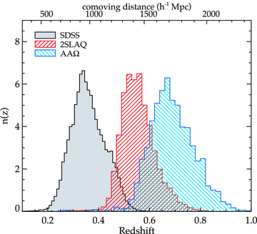
Normalized redshift distributions, n(z), of the three LRG spectroscopic surveys used as the basis for selection criteria in this study.

Open in new tabDownload slide

All magnitudes and colours are given in SDSS AB system and are corrected for extinction using the Galactic dust map of Schlegel, Finkbeiner & Davis (1998). In this analysis, we only used the galaxy samples in the most contiguous part of the survey, i.e. the northern Galactic cap (NGC). All colours described below refer to the differences in ‘model’ magnitudes (see Lupton et al. 2001, for a review on model magnitudes) unless otherwise stated.

Hereafter, we shall refer to the photometrically selected sample (not to be confused with the spectroscopic sample from which they are associated) at average redshift of 0.35, 0.55 and 0.7 as the ‘SDSS LRG’, ‘2SLAQ LRG’ and ‘AAΩ LRG’, respectively.

2.1 SDSS LRG

The sample used here is similar to the target sample of the recently completed SDSS-LRG spectroscopic survey which contains ≈100 000 spectra and cover over 1 h⁻³ Gpc³. These objects are classified as LRGs on the basis of their colours and magnitudes following E01. The sample is approximately volume-limited up to z≈ 0.38 and spans out to z≈ 0.5. The selection is done using (g−r) and (r−i) colours coupled with r-band (Petrosian 1976) magnitude system. The algorithm is designed to extract LRGs in two different (but slightly overlapped) regions of the gri colour space and hence using two selection criteria (Cut I and Cut II in E01) as naturally suggested by the locus of early-type galaxy on this colour plane (see Fig. 2). The tracks shown in Fig. 2 were constructed using a spectral evolution model of stellar populations (Bruzual & Charlot 2003) with output spectra mimicking a typical SED of the LRGs. The stellar populations were formed at z≈ 10 and then evolve with two different scenarios, namely (i) passive evolution of an instantaneous star formation (single burst), and (ii) exponentially decayed star formation rate (SFR) with e-folding time of 1 Gyr. Solar metallicity and Salpeter (1955) initial mass function (IMF) were assumed in both evolutionary models.

Figure 2

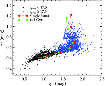
The colour–colour plot of SDSS LRG Cut I and II showing their positions on the gri colour plane compared to the predicted colour–colour locus (observer frame) of typical early-type galaxies as a function of redshift (see text for more details). Each solid circle denotes the redshift evolution of the colour–colour tracks at the interval of 0.1 beginning with z = 0.1 (bottom left).

Open in new tabDownload slide

We used the same colour–magnitude selection as that described by E01 but with additional restriction on the r-band apparent magnitudes of the objects, i.e. r_petro≥ 17.5. This is due mainly to two reasons, (i) to separate out the objects with z < 0.2 because Cut I is too permissive and allows under-luminous objects to enter the sample below redshift 0.2 as also emphasized by E01, and (ii) to tighten the redshift distribution of our sample while maintaining the number of objects and its average redshift (see Fig. 3).

Figure 3

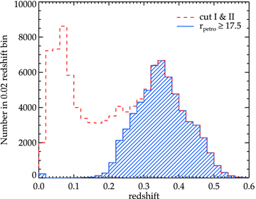
The number of objects as a function of redshift from SDSS-LRG spectroscopic redshift survey, also shown is the subset of Cut I and II with additional magnitude cut, r_petro≥ 17.5, applied.

Open in new tabDownload slide

The selection criteria mentioned above also have another star–galaxy separation algorithm apart from the pipeline PHOTO classification (Lupton et al. 2001). This was done by setting a lower limit on the differences in r-band point spread function (PSF) magnitudes and model magnitudes as most galaxies populate the upper part of r_PSF−r_model space compare to the foreground star of similar apparent magnitude. The algorithm has been proven to be quite effective (less than 1 per cent stellar contamination) for this range of redshift and magnitude although Cut II needs a more restrictive threshold, r_PSF−r_model > 0.5 as compared to 0.3 for Cut I.

In practice, the LRG sample described here can be extracted from the SDSS DR5 imaging data base using the Structured Query Language (SQL) query by setting the flag PRIMTARGET to GALAXY_RED. This yields a catalogue of approximately 200 000 objects which after applying the additional magnitude cut mentioned above becomes 106 699 objects and results in the sky surface density of about 13 objects per square degree.

2.2 2SLAQ LRG

The 2dF-SDSS LRG and Quasar Survey (2SLAQ) is the spectroscopic follow-up of intermediate- to high-redshift (z > 0.4) LRGs from photometric data of SDSS DR4 (Adelman-McCarthy et al. 2006) using the two-degree Field (2dF) instrument on the Anglo-Australian Telescope (AAT). This survey is now completed and contains approximately 13 000 bona fide LRGs with over 90 per cent at 0.45 < z < 0.8 in two narrow equatorial strips covering 180 deg². The primary sample of the survey (Sample 8; C06) was selected using (g−r) versus (r−i) colours and ‘de Vaucouleurs’i-band magnitude (17.5 < i_deV < 19.8). The colour selection of Sample 8 is similar to that of Cut II which utilizes the upturn of the early-type galaxy locus in gri colour plane and hence is immune against the confusion with the late-type galaxy locus at higher redshift (see fig. 2 in E01) but the scattering up in colour of interlopers from lower redshift and contamination of M-stars can also affect the accuracy of the selection. The latter could be prevented by using a similar method for star–galaxy separation as described in the last section but in this case we used the i-band magnitude rather than the r band. Following C06, two criteria were used,

1

and

2

where radius_deV(i) is de Vaucouleurs radius fit of the i-band photometry. As reported by C06, approximately 5 per cent of the cool dwarf M-stars are still present in their sample and we shall assume this value when correcting for the dilution of the correlation signal due to the uncorrelated nature of foreground stars and the LRGs. In this work, we only use Sample 8 as this provides us with a narrower n(z) and higher average redshift than the whole 2SLAQ sample.

A sample of 655 775 photometrically selected LRG candidates (≈5 per cent stellar contamination) is returned by the SDSS DR5 ‘Best Imaging’ data base when the Sample 8 selection criteria are used in the SQL query from table GALAXY. Objects with BRIGHT or SATURATED or BLENDED but not DEBLENDED flags are not included in our sample.

2.3 AAΩ LRG

The AAΩ-AAT LRG Pilot observing run was carried out in 2006 March by Ross et al. (2008a, and references therein) as a ‘Proof of Concept’ for a large spectroscopic redshift survey, VST-AAΩATLAS, using the new AAΩ instrument on the AAT. The survey was designed to target photometrically selected LRGs out to z≈ 1.0 with the average redshift of 0.7. The target sample was observed in three 2dF including the COSMOS field (Scoville et al. 2007), the COMBO-17 S11 field (Wolf et al. 2001), and 2SLAQ d05 field (C06).

We follow the survey main selection criteria, 19.8 < i_deV≤ 20.5, together with the riz colour cuts as described by Ross et al. (2008a). In summary, the cut utilizes the upturn of the early-type galaxy colour–colour locus similar to that used by 2SLAQ and SDSS-LRG surveys. The turning point of the track on the riz colour plane occurs at z = 0.6–0.7 as the 4000 Å feature moves from the SDSS r to i band whilst this happens at z≈ 0.4 in the gri case. The selection technique has been proven to work reasonably well by the observed redshift distribution. This is further confirmed by the ongoing AAT-AAΩ LRG project, the down-sized version of the VST-AAΩATLAS survey, designed to observe several thousands of LRG redshifts for photo-z calibration and a clustering evolution study. The n(z) (Fig. 1) used in inferring the 3D clustering information also includes ≈2000 AAΩ LRG redshifts taken during the run in June 2008.

As emphasized by Ross et al. (2008a), the stellar contamination in the sample can be readily reduced to ≈16 per cent by imposing star–galaxy separation in the z-band without any significant loss of genuine galaxies. Although the level of contamination could be further reduced by using near-infrared photometry, we do not attempt it here as there is no infrared survey that covers the entire SDSS DR5 NGC sky with similar depth. Therefore, we shall use the quoted contamination fraction when correcting the measured w(θ) for the same reason mentioned in Section 2.2. Since no expression for star–galaxy separation is given in Ross et al. (2008a), here such a procedure is performed using an equation defining the dashed line in their fig. 3,

3

Applying the above selection rules on the ‘Best Imaging’ data of the SDSS DR5 yields a photometric sample of 800 346 high-redshift LRG candidates with the sky surface density of approximately 110 objects per square degree. As with the 2SLAQ-LRG sample, objects with BRIGHT or SATURATED or BLENDED but not DEBLENDED flags are discarded from our sample.

3 ESTIMATING w(θ) AND ITS ERROR

3.1 Optimal estimator and techniques

The two-point correlation function, ξ(r), measures the excess probability of finding a pair of objects separated by distance r relative to that expected from a randomly distributed process. The joint probability of finding two objects of interest (in this case the LRGs) in the volume elements δV₁ and δV₂ separated by a distance r is given by

4

where n is the number space density of the sample. In practice, redshift of individual object is required to estimate the separation between a given pair. However if such redshift information is not available as in this study, the sky projected version, w(θ), can be used to analyse the clustering property of the sample instead. The 2D equivalent of equation (4) is

5

where ℵ is the surface density of the objects and δP(θ) is now the joint probability of finding two objects in solid angle δΩ₁ and δΩ₂ separated by angle θ.

Two possible routes for estimating w(θ) are the pixelization of galaxy number overdensity, and pair counting. The pixelization approach usually requires less computation time but its smallest scale probed is limited by the pixel size. We choose to follow the latter. To calculate w(θ) using the pair counting method, one usually generates a random catalogue whose angular selection function is described by the survey. The number of random points are generally required to be 10 times the number of objects or more. This is necessary to reduce the shot noise. Our random catalogue for each sample has ≈20 times the number of LRGs in SDSS and 10 times for 2SLAQ and AAΩ-pilot (see the next section for details on how this was achieved).

We compute w(θ) using the minimum variance estimator of Landy & Szalay (1993). It is also an unbiased estimator (Martínez & Saar 2002) for the two-point correlation function (2PCF) as it can be reduced to the exact theoretical definition of 2PCF, i.e. a variance of density fluctuation in Gaussian field, ξ (r) =〈δ (x) δ (x+r)〉. The form of this estimator is

6

where DD(θ) is the number of LRG–LRG pairs with angular separation within the angular bin centres at θ. DR(θ) and RR(θ) are the numbers of LRG–random and random–random pairs, respectively. The N_rd/N ratio is required for normalization. N_rd is the total number of random points and N is the total number of LRGs. We use a logarithmic binwidth of Δlog (θ/arcmin) = 0.176 for θ = 0.1 to 50 arcmin and a linear binwidth of 20 arcmin at scales larger than 50 arcmin.

The uncertainty in the number density of the sample could lead to a bias in the estimation of w(θ) when using the Landy–Szalay estimator especially at large scales where the amplitude is small and hence we also utilize the Hamilton (1993) estimator, given by

7

which requires no normalization. We used the Hamilton estimator to cross-check our w_LS for each sample and found the difference given by the two estimators to be negligible in all three samples.

For the purpose of determining statistical uncertainty in our measurement, three methods of estimating the errors are considered. The first method is the simple Poisson error given by

8

For the second method, field-to-field error, we split the sample into 24 subfields of approximately equal size. These subfields are large enough for estimating the correlation function up to the scale of interest. This is simply a standard deviation of the measurement in each subfield from the best estimate and is calculated using

9

where N is the total number of subfields, w_i(θ) is a measurement from the ith subfield and w(θ) is measured using the whole sample. The deviation of the angular correlation function computed in each subfield is weighted by DR_i(θ)/DR(θ) to account for their relative sizes.

The third method is the jackknife (JK) resampling. This is a method of preference in a number of correlation studies (see e.g. Scranton et al. 2002; Zehavi et al. 2005a; Ross et al. 2007). The JK errors are computed using the deviation of w(θ) measured from the combined 23 subfields out of the 24 subfields. The subfields are the same as used for the estimation of field-to-field error above. w(θ) is calculated repeatedly, each time leaving out a different subfield and hence results in a total of 24 measurements. The JK error is then

10

where is now an angular correlation function estimated using the whole sample except the ith subfield and is approximately 23/24 with slight variation depending on the size of the resampling field.

The w(θ) measured from a restricted area are known to suffer from a negative offset called ‘integral constraint’, ic, which tends to force the fluctuation on the scales of the survey to zero (Groth & Peebles 1977), i.e. w_est(θ) =w(θ) −ic. The integral constraint can be estimated from the random pair counts drawn from the same angular selection function (Section 3.2) as the data (see e.g. Roche & Eales 1999);

11

where we assume our fiducial ΛCDM model (see Section 4.2) for w_model. The ic for the SDSS, 2SLAQ and AAΩ-LRG samples are 4 × 10⁻⁴, 1.5 × 10⁻⁴ and 8 × 10⁻⁵, respectively. These are much smaller than the w(θ)’s amplitudes in the angular ranges being considered in this paper, as expected given the large sky coverage of the SDSS data.

It is well known that the correlation function bins are correlated which could affect the confidence limit on the parameter estimation performed under the assumption that each data point is independent. Comparison of the estimated error using the field-to-field and JK techniques to the simple Poisson error can give a rough estimate of the deviation from the independent point assumption. This is plotted in Fig. 4 which shows that the assumption is valid on small scales where Poisson error is a fair estimate of the statistical uncertainty. However the same cannot be said on large scales where the data points are correlated and the independent point assumption no longer holds. At these scales, such statistical uncertainty is likely to be dominated by edge-effects and cosmic variance.

Figure 4

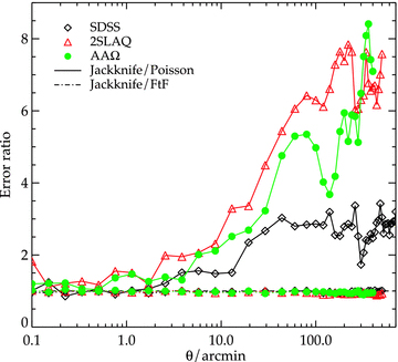
The ratio of JK to Poisson and field-to-field errors on the measurements of w(θ). The open diamonds, triangles and solid circles give the error ratios of w(θ) estimated from SDSS, 2SLAQ and AAΩ LRG, respectively.

Open in new tabDownload slide

Fig. 4 also shows that the errors estimated using field-to-field and JK methods are in good agreement at all angular scales except for 2SLAQ and AAΩ samples where the JK errors are slightly smaller towards the large scales but still agree within 10 per cent. The errors quoted in later sections are estimated using the JK resampling method.

The covariance matrix allows the correlation between each bin to be quantified and can be used in the fitting procedure to de-correlate the separation bins. We calculate the covariance matrix from the JK resampling using

12

where is the mean angular correlation function of all the JK subsamples in the jth bin. Note that the difference between and w(θ) estimated using the whole sample is negligible. We then proceed to compute the ‘correlation coefficient’, ⁠, defined by

13

Fig. 5 shows the correlation coefficients for the three samples which are strongly correlated at the largest scale considered and less at small scales confirming the simple correlation test using Poisson errors. Note that for the purpose of model fittings in the large-scale sections (Sections 4.2, 4.3 and 6) where a more stable covariance matrix is required, we increase the number of resampling fields to 96 subregions with approximately equal area. The size of these subregions is also big enough for the largest scale being considered in this paper. The correlation coefficients constructed from these 96 JK resampling are shown in Fig. A1 for the three LRG samples.

Figure 5

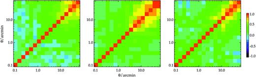
The correlation coefficients, ⁠, showing the level of correlation between each angular separation bin for SDSS, 2SLAQ and AAΩ LRG (left to right). Note that for each sample we only show up to the angular separation which corresponds to ≈20 h⁻¹ Mpc where later we shall attempt to fit power-law forms to the measured w(θ)s.

Open in new tabDownload slide

Figure A1

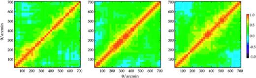
The correlation coefficients, ⁠, out to very large angular separations. These are derived from the covariance matrices (equation 13) via 96 JK re-sampling fields. Three panels show for SDSS, 2SLAQ and AAΩ-LRG samples from left to right.

Open in new tabDownload slide

We use the kd-trees code (Moore et al. 2001) to minimize the computation time required in the pair counting procedure. The angular correlation function is estimated using the method described above and then corrected for stellar contamination which reduce the amplitude by a factor (1 −f)², where f is the contamination fraction for each sample given in Section 2.

3.2 Constructing random catalogues

In order to calculate the angular correlation function accurately, a random catalogue is required. This catalogue consists of randomly distributed points with the total number at least 10 times that of the data. Each random point is assigned a position in Right Ascension (RA) and Declination (DEC). Since our sample spans a wide range in DEC (see Fig. 6 for the SDSS DR5 sky coverage), care must be taken to keep the surface number density constant assuming the survey completeness is constant and uniform throughout. Only the random points that satisfy the angular selection function of the survey as defined by the mask are selected.

Figure 6

An equal area Aitoff projection of a random catalogue described in Section 3.2. The red/grey highlighted regions indicate the areas where adjacent stripes are overlapped. Note that the shading is purely diagrammatic to show the overlap regions and is unrelated to galaxy density.

Open in new tabDownload slide

The mask is constructed from ‘BEST’ DR5 imaging sky coverage given2 in the survey coordinate (λ, η) and stripe number. The sky is drift scanned in a strip parallel to η and two strips are required to fill a stripe (York et al. 2000). Each stripe is wide and their centres are separated by ⁠. In addition to the ‘BEST’ sky coverage mask, we also exclude regions in the quality ‘holes’ and regions defined as ‘BLEEDING’, ‘BRIGHT_STAR’, ‘TRAIL’ and ‘HOLE’ in the ‘mask’ table given by the SDSS data base. The final mask is applied to both our data and random catalogues.

Note that further away from the survey equator (RA₂₀₀₀ = 185°), the adjacent stripes become overlapped which account for almost 20 per cent of the sky coverage. The ‘BEST’ imaging data base only keep the best photometry of the objects which have been detected more than once in the overlap regions. At the faint magnitude limit of our sample, this could lead to a higher completeness in the overlap region and introduces bias in the estimated correlation function. This issue has also been addressed by Blake et al. (2007). They compared the measurement from the sample which omits the overlap region against their best estimate and found no significant difference. We follow their approach by excluding the overlap regions and re-calculating the angular correlation function of our faintest apparent magnitude sample, AAΩ-LRG, where the issue is expected to be the most severe. We found no significant change compared to our best estimate using the whole sample.

3.3 Inferring 3D clustering

The angular correlation function estimated from the same population with the same clustering strength will have a different amplitude at a given angular scale if they are at different depths (redshifts) or have different redshift selection functions, ϕ(z). Therefore in order to accurately compare the clustering strengths of different samples inferred from w(θ), one needs to know the sample ϕ(z). Even if the redshifts of individual galaxies are not available, their 3D clustering information can be recovered if the sample redshift distribution, n(z), is known. The equation that relates the spatial coherence length, r₀, to the amplitude of w(θ) is usually referred to as Limber’s equation.

Recently, the accuracy of Limber’s equation has been called into question. This is due to the assumption made for Limber’s approximation that the selection function, ϕ(z), varies much more slowly than ξ(r) in addition to the flat-sky (small angle) approximation. It was shown by Simon (2007) that such an assumption would lead to w(θ) being overestimated at large angle where the breakdown scale becomes smaller for narrower ϕ(z) (see Fig. 7). Here, we shall use the relativistic generalization of Limber’s equation suggested by Phillipps et al. (1978) but without the approximation mentioned above. Following Phillipps et al. (1978) for the comoving case,

14

The source’s radial distribution, f(z), is simply given by the galaxy selection function, ϕ(z), as

15

where χ is the radial comoving distance, n_c(z) is the comoving number density of the sources and r=r(θ, z₁, z₂) is a comoving separation of the galaxy pair. We shall assume a spatially flat cosmology (see Section 4.2) hence

16

Note that equation (14) can also be used to relate a non-power-law spatial correlation function to w(θ) unlike the conventional power-law approximation of Limber’s equation (Phillipps et al. 1978).

Figure 7

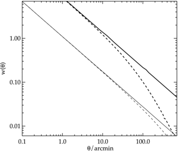
The angular correlation function computed using the full (dashed-lines) and approximate (solid-lines) Limber equation, derived using a power law, ξ(r) = (r/r₀)^−γ where r₀ = 10 h⁻¹ Mpc and γ = 1.8 with the SDSS LRG n(z) for the thin lines and much narrower n(z) (±0.01 centred at z = 0.35) for the thick lines.

Open in new tabDownload slide

Fig. 7 shows w(θ) computed using equation (14) (dashed lines) compared to the conventional Limber’s approximation (solid lines) for a power-law ξ(r) with clustering length 10 h⁻¹ Mpc and γ = 1.8. The effect of a much narrower redshift distribution (thick lines) is also shown where the break scale becomes smaller and the power-law slope of w(θ) asymptotically approaches that of ξ(r), agreeing with the finding of Simon (2007). We shall use equation (14) together with the known n(z) to infer the 3D spatial clustering of the LRGs.

4 RESULTS

4.1 Power-law fits

We first look at the angular correlation function measured from the LRG sample at scales less than 1° corresponding to approximately 20 h⁻¹ Mpc where previous studies suggested that the spatial 2PCF can be described by a single power law of the form ξ(r) = (r/r₀)^−γ (typically γ = 1.8) and a single power-law w(θ) with slope 1 −γ is expected (see Fig. 7). However in this study, we find a deviation from a single power law with a break in the slope at ≈1 h⁻¹ Mpc in all three samples (less significant for the SDSS LRG). The measurement has a steeper slope at small scales (<1 h⁻¹ Mpc) and is slightly flatter on scales up to ≈20 h⁻¹ Mpc where it begins to drop sharply (see Figs 8 and 9). The inflexion feature at ≈1 h⁻¹ Mpc has also been reported in the spatial and semi-projected, w_p(σ), correlation function by many authors (e.g. Zehavi et al. 2005a; Phleps et al. 2006; Ross et al. 2007; Blake et al. 2008) and detections go back as far as Shanks et al. (1983). We shall return to discuss these features in the halo model framework (Section 4.3).

Figure 8

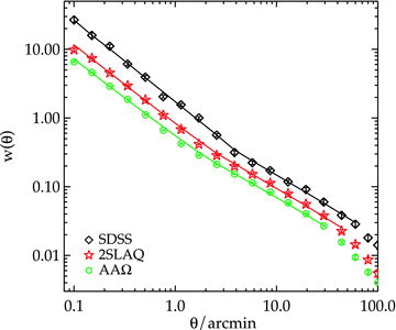
The angular correlation function measured from the three LRG samples. The solid lines are the projection of best-fitting double power-law ξ(r) with r₀ and γ given in Table 2 for each sample. The break scales occur at approximately a few arcmin depending on the average redshift of the sample. This corresponds to a comoving separation of ≈1 h⁻¹ Mpc (see Fig. 9).

Open in new tabDownload slide

Figure 9

The angular correlation function with the best-fitting single (red dashed line) and double (blue solid line) power law for the SDSS, 2SLAQ and AAΩ LRGs. Lower panels show the fitting residuals for the single (circles) and double (triangles) power law.

Open in new tabDownload slide

If we first consider w(θ) at scales smaller and larger than the break point separately, each can be approximately described by a power law with a slope of ≈−1.15 (γ = 2.15), and ≈−0.83 (γ = 1.83), respectively. A more detailed analysis is performed by fitting a set of models to the measured w(θ) using a chi-squared minimization method with the full covariance matrix constructed from the JK resampling (see Section 3.1). This allows us to quantify the significance of the deviation from the single power law by comparing its goodness of fit to a double power law. We proceed by calculating

17

where N is the number of angular bins, Δw(θ_i) is the difference between the measured angular correlation function and the model for the ith bin, and is the inverse of covariance matrix.

The single power-law fit is of the form w(θ) = (θ/θ₀)^{(1 −γ)}. We also recover the spatial clustering length, r₀, and its slope through the fitting via equation (14). For a double power law, the fitting procedure is performed separately at the scales smaller and larger than θ_b, corresponding to ≈1 h⁻¹ Mpc for all three samples (see Fig. 9). The largest scale considered in the fitting for all cases is ≈20 h⁻¹ Mpc where a steeper drop-off of w(θ) is observed.

In Fig. 9, the best-fitting power laws for all three samples are shown. The summary of the best-fitting parameters is given in Table 2. Equations (14) and (17) are then used to find the spatial clustering lengths and slopes that best describe our w(θ) results. The best-fitting clustering slopes from r₀−γ analysis using Limber’s equation are in good agreement with that from θ₀−γ and hence we only report the latter in Table 2. If we require continuity in the double power-law ξ(r) at the break scale, such a scale can be constrained by the pair of best-fitting r₀-γ for each sample. From Table 2, the double power-law break for the SDSS, 2SLAQ and AAΩ samples is then at 2.2, 1.9 and 1.3 h⁻¹ Mpc, respectively [see Section 5.2 for further discussion of the possible small-scale evolution of ξ(r)]. By assuming the 1 h⁻¹ Mpc break instead of aforementioned values, the w(θ) is underestimated by ≈10 per cent for the SDSS case (less for the other two samples) which is only localized to around θ_b. The clustering length (single power law), r₀, ranges from 7.5 to 8.7 h⁻¹ Mpc, consistent with highly biased luminous galaxies. Single power-law fits to the data can be ruled out at high statistical significance. While the double power law gives better fits to the data than the single power law, their χ²_red values indicate that such a model is still not a good fit to the data, given the small statistical errors. Nevertheless, to the first order, the double power-law fits provide a good way of quantifying the spatial clustering strength of the samples via the use of Limber’s equation.

Table 2

Open in new tab

Parameters for the power-law fits to the angular correlation function derived from three LRG samples. The best-fitting parameters given are defined such that w(θ) = (θ/θ₀)^{1 −γ} and ξ(r) = (r/r₀)^−γ. The parameters for the best-fitting double power law are given in two rows whereas the θ < θ_b result is given in the top row. Also given are the corresponding 1σ error for each parameter.

Sample		ng (h3 Mpc−3)	Single power law				Double power law			χ2red
			θ0(arcmin)	γ	r0(h−1 Mpc)	χ2red	θ0(arcmin)	γ	r0(h−1 Mpc)
SDSS	0.35	1.1 × 10−4	1.69 ± 0.03	2.07 ± 0.01	8.70 ± 0.09	16.2	1.57 ± 0.05	2.19 ± 0.03	7.35 ± 0.08	2.2
							1.05 ± 0.09	1.85 ± 0.04	9.15 ± 0.16
2SLAQ	0.55	3.2 × 10−4	0.87 ± 0.01	2.01 ± 0.01	7.50 ± 0.04	57.5	0.83 ± 0.01	2.16 ± 0.01	6.32 ± 0.03	3.9
							0.60 ± 0.03	1.84 ± 0.02	7.78 ± 0.05
AAΩ	0.68	2.7 × 10−4	0.57 ± 0.01	1.96 ± 0.01	7.56 ± 0.03	42.8	0.56 ± 0.01	2.14 ± 0.01	5.96 ± 0.03	3.4
							0.38 ± 0.02	1.81 ± 0.02	7.84 ± 0.04

Sample		ng (h3 Mpc−3)	Single power law				Double power law			χ2red
			θ0(arcmin)	γ	r0(h−1 Mpc)	χ2red	θ0(arcmin)	γ	r0(h−1 Mpc)
SDSS	0.35	1.1 × 10−4	1.69 ± 0.03	2.07 ± 0.01	8.70 ± 0.09	16.2	1.57 ± 0.05	2.19 ± 0.03	7.35 ± 0.08	2.2
							1.05 ± 0.09	1.85 ± 0.04	9.15 ± 0.16
2SLAQ	0.55	3.2 × 10−4	0.87 ± 0.01	2.01 ± 0.01	7.50 ± 0.04	57.5	0.83 ± 0.01	2.16 ± 0.01	6.32 ± 0.03	3.9
							0.60 ± 0.03	1.84 ± 0.02	7.78 ± 0.05
AAΩ	0.68	2.7 × 10−4	0.57 ± 0.01	1.96 ± 0.01	7.56 ± 0.03	42.8	0.56 ± 0.01	2.14 ± 0.01	5.96 ± 0.03	3.4
							0.38 ± 0.02	1.81 ± 0.02	7.84 ± 0.04

Table 2

Open in new tab

Parameters for the power-law fits to the angular correlation function derived from three LRG samples. The best-fitting parameters given are defined such that w(θ) = (θ/θ₀)^{1 −γ} and ξ(r) = (r/r₀)^−γ. The parameters for the best-fitting double power law are given in two rows whereas the θ < θ_b result is given in the top row. Also given are the corresponding 1σ error for each parameter.

Sample		ng (h3 Mpc−3)	Single power law				Double power law			χ2red
			θ0(arcmin)	γ	r0(h−1 Mpc)	χ2red	θ0(arcmin)	γ	r0(h−1 Mpc)
SDSS	0.35	1.1 × 10−4	1.69 ± 0.03	2.07 ± 0.01	8.70 ± 0.09	16.2	1.57 ± 0.05	2.19 ± 0.03	7.35 ± 0.08	2.2
							1.05 ± 0.09	1.85 ± 0.04	9.15 ± 0.16
2SLAQ	0.55	3.2 × 10−4	0.87 ± 0.01	2.01 ± 0.01	7.50 ± 0.04	57.5	0.83 ± 0.01	2.16 ± 0.01	6.32 ± 0.03	3.9
							0.60 ± 0.03	1.84 ± 0.02	7.78 ± 0.05
AAΩ	0.68	2.7 × 10−4	0.57 ± 0.01	1.96 ± 0.01	7.56 ± 0.03	42.8	0.56 ± 0.01	2.14 ± 0.01	5.96 ± 0.03	3.4
							0.38 ± 0.02	1.81 ± 0.02	7.84 ± 0.04

Sample		ng (h3 Mpc−3)	Single power law				Double power law			χ2red
			θ0(arcmin)	γ	r0(h−1 Mpc)	χ2red	θ0(arcmin)	γ	r0(h−1 Mpc)
SDSS	0.35	1.1 × 10−4	1.69 ± 0.03	2.07 ± 0.01	8.70 ± 0.09	16.2	1.57 ± 0.05	2.19 ± 0.03	7.35 ± 0.08	2.2
							1.05 ± 0.09	1.85 ± 0.04	9.15 ± 0.16
2SLAQ	0.55	3.2 × 10−4	0.87 ± 0.01	2.01 ± 0.01	7.50 ± 0.04	57.5	0.83 ± 0.01	2.16 ± 0.01	6.32 ± 0.03	3.9
							0.60 ± 0.03	1.84 ± 0.02	7.78 ± 0.05
AAΩ	0.68	2.7 × 10−4	0.57 ± 0.01	1.96 ± 0.01	7.56 ± 0.03	42.8	0.56 ± 0.01	2.14 ± 0.01	5.96 ± 0.03	3.4
							0.38 ± 0.02	1.81 ± 0.02	7.84 ± 0.04

The best-fitting slopes at small scales show a slight decrease with increasing redshift, similar to that found by Wake et al. (2008). The SDSS-LRG sample is more strongly clustered than the rest as expected. This is simply because the SDSS-LRG sample is intrinsically more luminous than the 2SLAQ and AAΩ-LRG samples, and is not an indication of evolution.

The galaxy number density (see Table 2) is calculated from the unnormalized n(z), assuming the redshift distribution from the spectroscopic surveys as described in Section 2. This is galaxy pair-weighted by n²(z) (see e.g. Ross & Brunner 2009)

18

where Ω_obs is the observed area of the sky, χ(z) is the comoving distance to redshift z and c is the speed of light. The samples’ pair-weighted average redshifts determined in the similar manner as n_g are consistent with their median redshifts and are given in Table 2.

To this end, we cut back the faint magnitude limit of 2SLAQ and AAΩ LRGs to i_deV < 19.32 and 20.25, respectively. These cuts are imposed in order to select the samples of galaxies whose comoving number densities are approximately matched to that of the SDSS LRG. The K+e corrected i-band absolute magnitudes of these samples are presented in Fig. 10. We see that their absolute magnitudes are also approximately matched. We note that we do not attempt to match the LRGs’ colour of different samples here. This would then allow us to roughly constrain the evolution of LRG clustering up to z≈ 0.68 (see Section 5). A summary of the properties of these samples and the best-fitting parameters is given in Table 3. The measured w(θ)s are shown in Fig. 11(a).

Figure 10

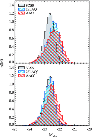
Top: the i-band absolute magnitude distribution of the spectroscopic LRG catalogues. All photometry is galactic-extinction corrected using dust map of Schlegel et al. (1998) and K+e corrected to z = 0 using the early-type galaxy templates from Bruzual & Charlot (2003). Bottom: the distribution of the absolute magnitude after applying a faint limit cut to 2SLAQ and AAΩ LRG in order to match the comoving number density of the SDSS LRG.

Open in new tabDownload slide

Table 3

Open in new tab

Properties and the best-fitting parameters for double power law of w(θ) measured from the SDSS-density matched samples.

Sample	Number	Magnitude		ng (h3 Mpc−3)	Double power law
					γ	r0(h−1 Mpc)	χ2red
2SLAQ*	182 841	17.5 < ideV < 19.32	0.53	1.2 × 10−4	2.25 ± 0.02	6.33 ± 0.04	2.1
					1.80 ± 0.02	8.88 ± 0.08
AAΩ*	374 198	19.8 < ideV < 20.25	0.67	1.1 × 10−4	2.20 ± 0.02	6.25 ± 0.03	1.7
					1.76 ± 0.03	9.08 ± 0.06

Sample	Number	Magnitude		ng (h3 Mpc−3)	Double power law
					γ	r0(h−1 Mpc)	χ2red
2SLAQ*	182 841	17.5 < ideV < 19.32	0.53	1.2 × 10−4	2.25 ± 0.02	6.33 ± 0.04	2.1
					1.80 ± 0.02	8.88 ± 0.08
AAΩ*	374 198	19.8 < ideV < 20.25	0.67	1.1 × 10−4	2.20 ± 0.02	6.25 ± 0.03	1.7
					1.76 ± 0.03	9.08 ± 0.06

Table 3

Open in new tab

Properties and the best-fitting parameters for double power law of w(θ) measured from the SDSS-density matched samples.

Sample	Number	Magnitude		ng (h3 Mpc−3)	Double power law
					γ	r0(h−1 Mpc)	χ2red
2SLAQ*	182 841	17.5 < ideV < 19.32	0.53	1.2 × 10−4	2.25 ± 0.02	6.33 ± 0.04	2.1
					1.80 ± 0.02	8.88 ± 0.08
AAΩ*	374 198	19.8 < ideV < 20.25	0.67	1.1 × 10−4	2.20 ± 0.02	6.25 ± 0.03	1.7
					1.76 ± 0.03	9.08 ± 0.06

Sample	Number	Magnitude		ng (h3 Mpc−3)	Double power law
					γ	r0(h−1 Mpc)	χ2red
2SLAQ*	182 841	17.5 < ideV < 19.32	0.53	1.2 × 10−4	2.25 ± 0.02	6.33 ± 0.04	2.1
					1.80 ± 0.02	8.88 ± 0.08
AAΩ*	374 198	19.8 < ideV < 20.25	0.67	1.1 × 10−4	2.20 ± 0.02	6.25 ± 0.03	1.7
					1.76 ± 0.03	9.08 ± 0.06

Figure 11

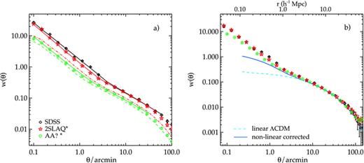
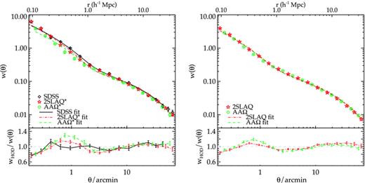
(a) The angular correlation function measured from the SDSS LRG and the brighter magnitude limit samples drawn from 2SLAQ and AAΩ sample (symbols). The solid lines are the projection of the best-fitting double power-law ξ(r) with the parameters shown in Table 3. For comparison, the dot–dashed and dashed lines are w(θ) measured from the whole 2SLAQ and AAΩ samples, respectively. (b) Same as (a) but now scaled to AAΩ depth and taking into account the relative amplitude due to the different n(z) widths (see text for more details).

Open in new tabDownload slide

As expected, the amplitudes of the brighter cut 2SLAQ and AAΩ samples (denoted by 2SLAQ* and AAΩ* hereafter) are higher than the original sample. In its raw form, w(θ) measured from 2SLAQ* increases relative to 2SLAQ more than AAΩ relative to AAΩ*, due to the narrower redshift distribution of the 2SLAQ* sample. However, if we perform a double power-law fit to these results, the large-scale, ≳1 h⁻¹ Mpc, clustering lengths are very similar and agree within ≈1σ statistical error. To the first order these large-scale clustering lengths are also consistent with that of the SDSS LRGs. We shall investigate the clustering evolution of these LRG samples further in Section 5.

4.2 Comparison of the clustering form to the standard ΛCDM model

We shall compare our w(θ) measurements to the predictions of the standard ΛCDM model in the linear perturbation theory of structure growth framework along with the non-linear correction. For the theoretical models, we first generate matter power spectra, using the ‘camb’ software (Lewis, Challinor & Lasenby 2000). In the case of non-linear correction, the software has the ‘halofit’ routine (Smith et al. 2003) implemented. Such matter power spectra, P_m(k, z), are then output at the average redshift of each sample. The matter correlation function, ξ_m(r), is then obtained by Fourier transforming these matter power spectra using

19

Under the assumption that galaxies trace dark matter haloes, the galaxy correlation function, ξ_g(r), is related to the underlying dark matter by the bias factor, b_g, via

20

Therefore, the bias factor is expected to be a function of scale unless galaxies cluster in exactly the same manner as the dark matter does at all scales. However, at large scales, i.e. the linear regime, the bias factor is approximately scale-independent over almost a decade of scales (Verde et al. 2002; Ross, Brunner & Myers 2008b).

Although we found the clustering lengths and hence the amplitude of ξ(r) to be very similar for the SDSS, 2SLAQ* and AAΩ* samples, the evolution in the dark matter clustering means that the linear bias could be a strong function of redshift as we shall see in the next section where we investigate the clustering evolution in more detail. The evolution of structures in linear theory framework is described by the linear growth factor, D(z) (e.g. Peebles 1984; Carroll, Press & Turner 1992) such that

21

recall that ⁠, where r = |r₁−r₂ |, then

22

The linear growth factor is unity at the present epoch, by definition, and decreases as a function of redshift. The ξ_m(r, z) therefore decreases as the redshift increases hence given that the number-density/luminosity-matched samples have similar ξ_g(r) amplitudes suggests that the bias increases as a function of redshift.

We proceed by projecting the predicted ξ_m(r) using equation (14). Our fiducial models assume a ΛCDM Universe with Ω_Λ = 0.73, Ω_m = 0.27, f_baryon = 0.167, σ₈ = 0.8, h = 0.7 and n_s = 0.95. The linear bias factor is then estimated by fitting the matter w(θ) to our measurements for the comoving separation of ≈ 6–60 h⁻¹ Mpc, using the full covariance matrices. The best-fitting linear bias (χ²_red) for SDSS, 2SLAQ*, AAΩ*, 2SLAQ and AAΩ samples are 2.09 ± 0.05(1.2), 2.20 ± 0.04(0.65), 2.33 ± 0.03(0.66), 1.98 ± 0.03(0.53) and 2.07 ± 0.02(1.2), respectively. The measured biases are consistent with the results from other authors. For example, Tegmark et al. (2006) analysed P(k) of SDSS LRG and found b(z = 0.35) = 2.25 ± 0.08 for the best-fitting σ₈ = 0.756 ± 0.035 and for our fiducial σ₈ this becomes b = 2.12 ± 0.12. Ross et al. (2007) found 2SLAQ LRG b = 1.66 ± 0.35 using the redshift-space distortion analysis. Padmanabhan et al. (2007), using C(l) of SDSS+2SLAQ photo-z sample, found that b(z = 0.376) = 1.94 ± 0.06 and b(z = 0.55) = 1.8 ± 0.04 (assumed σ₈ = 0.9), for our fiducial σ₈ these are b = 2.18 ± 0.07 and b = 2.02 ± 0.05, respectively.

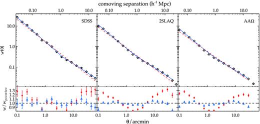
Fig. 11(b) shows the full scaling of the w(θ)s, accounting for their survey differences. First, the w(θ) of the SDSS, and 2SLAQ* samples scaled in the angular direction according to their average redshifts and relative to the AAΩ* sample. The amplitudes are then scaled to obtain a fair comparison for samples with different redshift distributions. This is done by taking the relative amplitudes of the projections of a power-law ξ(r) of the same clustering strength but projected through different n(z) widths. Since the observed large-scale clustering lengths are very similar, ≈9 h⁻¹ Mpc, the scaled w(θ)s in these ranges agree reasonably well. The figure also shows the best-fitting biased non-linear model for the AAΩ* sample. Our w(θ) shapes in the ranges 6 ≲r≲ 60 h⁻¹ Mpc can be described very well by the perturbation theory in the standard flat ΛCDM Universe (see the χ²_red for the best-fitting bias factor given above). However, at smaller scales the theory underestimates the clustering amplitude, as expected for early-type galaxies. As we shall see in Section 4.3, the reason for this may lie in the details of how the LRGs populate their dark matter halo hosts.

4.3 Halo model fits

We fit a halo model (e.g. Peacock & Smith 2000; Berlind & Weinberg 2002; Cooray & Sheth 2002) to our angular correlation function results. One of the key ingredients of the halo model is the halo occupation distribution (HOD) which tells us how the galaxies populate dark matter haloes as a function of halo mass. Recently, the model has been used to fit various data sets as a means to physically interpret the galaxy correlation function and gain insight into their evolution (e.g. White et al. 2007; Blake et al. 2008; Brown et al. 2008; Wake et al. 2008; Ross & Brunner 2009; Zheng et al. 2009).

Here, we use a three-parameter HOD model (e.g. Seo, Eisenstein & Zehavi 2008; Wake et al. 2008) which distinguishes between the central and satellite galaxies in a halo (Kravtsov et al. 2004). The mean number of galaxies residing in a halo of mass M is

23

where the number of central galaxy is either zero or one with the mean given by

24

We assume that only haloes with a central galaxy are allowed to host satellite galaxies. In such a halo, the satellite galaxies are distributed following an NFW profile (Navarro, Frenk & White 1997) around a central galaxy at the centre of the halo. We also assume that their numbers follow a Poisson distribution (Kravtsov et al. 2004) with a mean

25

The NFW profile is parametrized by the concentration parameter c≡r_vir/r_s where r_vir is the virial radius and r_s is the characteristic scale radius. We assume Bullock et al. (2001) parametrization of the halo concentration as a function of mass and redshift,

26

where M_* is the typical collapsing mass and is determined by solving equation (42) with σ(M_*) =δ_c(0).

The galaxy number density predicted by a given HOD is then

27

where n(M) is the halo mass function; here we use the model given by Sheth & Lemson (1999). The effective galaxy linear bias can be determined from the HOD;

28

where b(M) is the halo bias as a function of mass, for which we use the model of Sheth, Mo & Tormen (2001) plus the improved parameters of Tinker et al. (2005) (see Section 5.1.2, equation 41). The average mass of haloes hosting such a galaxy population is then

29

Moreover, the satellite fraction of the galaxy population is given by

30

The galaxy power spectrum/correlation function can then be modelled as having a contribution at small scales that arises from galaxy pairs in the same dark matter halo (one-halo term). On the other hand, the galaxy pairs in two separate haloes (two-halo term) dominate at larger scales,

31

The one-halo term can be distinguished into central–satellite, P_cs(k), and satellite–satellite, P_ss(k), contributions (see e.g. Skibba & Sheth 2009);

32

and

33

where u(k, M) is the Fourier transform of the NFW profile, and we have simplified the number of satellite–satellite pairs 〈N_s(N_s− 1)〉 to 〈N_s(M)〉², i.e. Poisson distribution.

For two-halo term, we implement the halo exclusion, ‘n′_g-matched’, and scale-dependent halo bias, b(M, r), of Tinker et al. (2005);

34

where P_m(k) is a non-linear matter power spectrum (see Section 4.2), M_lim(r) is the mass limit at separation r due to halo exclusion and n′_g is the restricted galaxy number density (equation B13 of Tinker et al. 2005). The scale-dependent halo bias is given by (Tinker et al. 2005)

35

where ξ_m is the non-linear correlation function (see Section 4.2).

The galaxy correlation function is then the Fourier transform of the power spectrum which can be calculated separately for one- and two-halo terms. For the two-halo term, we need to correct the galaxy pairs from the restricted galaxy density to the entire galaxy population. This is done by

36

where ξ′_2h(r) is the Fourier transform of equation (34).

We then project the predicted galaxy correlation function to w(θ) using equation (14) for a range of HOD parameters. The best-fitting model for each of our sample is then determined from chi-square minimization using the full covariance matrix. Note that we exclude angular bins corresponding to scales smaller than 0.1 h⁻¹ Mpc because any uncertainty in the ξ(r) model at very small scales, r≲ 0.01 h⁻¹ Mpc, can have a strong effect on w(θ) even at these scales due to the projection. The best-fitting M_min, M₁ and α and the associated values for n_g, M_eff, F_sat and b_lin are given in Table 4. The 1σ uncertainties on the best-fitting M_min, M₁ and α are determined from the parameter space where Δχ²≤ 1. For n_g, M_eff, F_sat and b_lin which depend on the three main HOD parameters, this becomes Δχ²≤ 3.53. Fig. 12 shows the best-fitting HOD for each sample; the coloured solid lines are the mean number of LRGs per halo with the central and satellite contributions shown separately as the dashed and dotted lines, respectively.

Table 4

Open in new tab

Best-fitting HOD parameters.

Sample		Mmin (1013h−1 M⊙)	M1 (1013h−1 M⊙)	α	ng (10−4h3 Mpc−3)	Meff (1013h−1 M⊙)	Fsat (per cent)	blin	χ2red
SDSS	0.35	2.5 ± 0.2	29.5 ± 2.5	1.58 ± 0.04	1.3 ± 0.4	6.4 ± 0.5	8.1 ± 1.8	2.08 ± 0.05	3.1
2SLAQ*	0.53	2.2 ± 0.1	27.3 ± 2.0	1.49 ± 0.03	1.3 ± 0.3	4.7 ± 0.2	7.0 ± 0.8	2.21 ± 0.04	7.7
AAΩ*	0.67	2.1 ± 0.1	23.8 ± 2.0	1.76 ± 0.04	1.2 ± 0.2	4.3 ± 0.2	5.7 ± 0.7	2.36 ± 0.04	10.1
2SLAQ	0.55	1.10 ± 0.07	13.6 ± 1.1	1.42 ± 0.02	3.2 ± 0.5	3.4 ± 0.2	10.0 ± 1.1	1.97 ± 0.03	14.2
AAΩ	0.68	1.02 ± 0.03	12.6 ± 1.0	1.50 ± 0.03	3.1 ± 0.4	3.0 ± 0.1	9.0 ± 0.09	2.08 ± 0.03	13.6

Sample		Mmin (1013h−1 M⊙)	M1 (1013h−1 M⊙)	α	ng (10−4h3 Mpc−3)	Meff (1013h−1 M⊙)	Fsat (per cent)	blin	χ2red
SDSS	0.35	2.5 ± 0.2	29.5 ± 2.5	1.58 ± 0.04	1.3 ± 0.4	6.4 ± 0.5	8.1 ± 1.8	2.08 ± 0.05	3.1
2SLAQ*	0.53	2.2 ± 0.1	27.3 ± 2.0	1.49 ± 0.03	1.3 ± 0.3	4.7 ± 0.2	7.0 ± 0.8	2.21 ± 0.04	7.7
AAΩ*	0.67	2.1 ± 0.1	23.8 ± 2.0	1.76 ± 0.04	1.2 ± 0.2	4.3 ± 0.2	5.7 ± 0.7	2.36 ± 0.04	10.1
2SLAQ	0.55	1.10 ± 0.07	13.6 ± 1.1	1.42 ± 0.02	3.2 ± 0.5	3.4 ± 0.2	10.0 ± 1.1	1.97 ± 0.03	14.2
AAΩ	0.68	1.02 ± 0.03	12.6 ± 1.0	1.50 ± 0.03	3.1 ± 0.4	3.0 ± 0.1	9.0 ± 0.09	2.08 ± 0.03	13.6

Table 4

Open in new tab

Best-fitting HOD parameters.

Sample		Mmin (1013h−1 M⊙)	M1 (1013h−1 M⊙)	α	ng (10−4h3 Mpc−3)	Meff (1013h−1 M⊙)	Fsat (per cent)	blin	χ2red
SDSS	0.35	2.5 ± 0.2	29.5 ± 2.5	1.58 ± 0.04	1.3 ± 0.4	6.4 ± 0.5	8.1 ± 1.8	2.08 ± 0.05	3.1
2SLAQ*	0.53	2.2 ± 0.1	27.3 ± 2.0	1.49 ± 0.03	1.3 ± 0.3	4.7 ± 0.2	7.0 ± 0.8	2.21 ± 0.04	7.7
AAΩ*	0.67	2.1 ± 0.1	23.8 ± 2.0	1.76 ± 0.04	1.2 ± 0.2	4.3 ± 0.2	5.7 ± 0.7	2.36 ± 0.04	10.1
2SLAQ	0.55	1.10 ± 0.07	13.6 ± 1.1	1.42 ± 0.02	3.2 ± 0.5	3.4 ± 0.2	10.0 ± 1.1	1.97 ± 0.03	14.2
AAΩ	0.68	1.02 ± 0.03	12.6 ± 1.0	1.50 ± 0.03	3.1 ± 0.4	3.0 ± 0.1	9.0 ± 0.09	2.08 ± 0.03	13.6

Sample		Mmin (1013h−1 M⊙)	M1 (1013h−1 M⊙)	α	ng (10−4h3 Mpc−3)	Meff (1013h−1 M⊙)	Fsat (per cent)	blin	χ2red
SDSS	0.35	2.5 ± 0.2	29.5 ± 2.5	1.58 ± 0.04	1.3 ± 0.4	6.4 ± 0.5	8.1 ± 1.8	2.08 ± 0.05	3.1
2SLAQ*	0.53	2.2 ± 0.1	27.3 ± 2.0	1.49 ± 0.03	1.3 ± 0.3	4.7 ± 0.2	7.0 ± 0.8	2.21 ± 0.04	7.7
AAΩ*	0.67	2.1 ± 0.1	23.8 ± 2.0	1.76 ± 0.04	1.2 ± 0.2	4.3 ± 0.2	5.7 ± 0.7	2.36 ± 0.04	10.1
2SLAQ	0.55	1.10 ± 0.07	13.6 ± 1.1	1.42 ± 0.02	3.2 ± 0.5	3.4 ± 0.2	10.0 ± 1.1	1.97 ± 0.03	14.2
AAΩ	0.68	1.02 ± 0.03	12.6 ± 1.0	1.50 ± 0.03	3.1 ± 0.4	3.0 ± 0.1	9.0 ± 0.09	2.08 ± 0.03	13.6

Figure 12

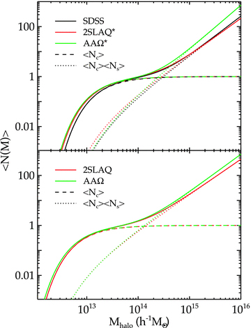
The mean number of LRGs per halo as a function of mass (solid lines) from the best-fitting HOD for the SDSS, 2SLAQ*, AAΩ* samples (top) and 2SLAQ, AAΩ samples (bottom). The central and satellite contributions for each sample are shown as the dashed and dotted lines.

Open in new tabDownload slide

As expected, the LRGs populate rather massive dark matter haloes with the masses ≈10¹³–10¹⁴h⁻¹ M_⊙. At approximately the same redshift, the more luminous samples, 2SLAQ* and AAΩ*, are hosted by more massive haloes than fainter samples. Most of the LRGs, >90 per cent, are central galaxies in their dark matter haloes; the satellite fraction is only 10 per cent or less with the increasing trend towards low redshift. This can be explained in the framework of halo mergers at lower redshift (see Section 5.2.2). The best-fitting linear bias factors for all samples are in excellent agreement with the values derived in Section 4.2. Also the galaxy number density from the best-fitting halo model is consistent with that derived from equation (18) (see Tables 2 and 3).

Note that, to the first order, our best-fitting HODs are compatible with the measurements from other authors although a direct comparison with samples selected differently may not be simple. For example, our SDSS sample has similar space density (although at higher redshift, z = 0.35 versus 0.3) as the sample studied by Seo et al. (2008). Our M₁/M_min and satellite fraction are in excellent agreement with their model 11 (their best-fitting N-body evolved HOD). But their α is somewhat lower which is caused by the higher σ₈ = 0.9 value (Wake et al. 2008) and the lower average redshift. Their M₁ and M_min are also somewhat higher than our best-fitting values for the same reason as for α. Another example, our best-fitting M₁, M_min, b_lin and F_sat for 2SLAQ* sample are in good agreement with Wake et al. (2008)z = 0.55 2SLAQ selection, although our values are somewhat higher which may be due to our lower galaxy number density, implying that our sample contains rarer and more biased objects.

The best-fitting models for w(θ) are shown in Fig. 13, comparing to the data. Both the models and data are scaled to account for the projection effect (see Section 4.2) and are plotted at the depth of AAΩ*/AAΩ sample. We immediately see that while the fits at the large scales (r≳ 3 h⁻¹ Mpc) are good, the fits at the small scales and at r≈ 1 − 2 h⁻¹ Mpc are rather poor especially for the higher redshift samples. This is evident in the high best-fitting reduced chi-square values in Table 4. Given our small error bars, this may indicate that a more complicated halo model may be needed, e.g. five/six parameters HOD, an improved halo-exclusion model (see fig. 11 of Tinker et al. 2005), or different halo concentration parametrization. Another important point to note is that the HOD formalism assumes a volume-limited sample, which we do not have here. This means that our observed galaxy number density corresponds to a cut-off which evolves with redshift rather than a cut-off in halo mass or LRG luminosity. Nevertheless, to the first order the HOD fits generally describe the shape and amplitude of our measured w(θ), and we believe that the derived b_lin and M_eff are reasonably robust despite the statistically poor fits.

Figure 13

The best-fitting HOD models for the SDSS, 2SLAQ*, AAΩ* samples (left) and 2SLAQ, AAΩ samples (right). These are scaled to the AAΩ*/AAΩ depth similar to that shown in Fig. 11(b). The bottom panels show the ratios between the best-fitting HOD models and the measured correlation functions.

Open in new tabDownload slide

5 EVOLUTION OF LRG CLUSTERING AND DARK MATTER HALO MASSES

5.1 Intermediate scales

We study the LRGs clustering and dark matter halo mass evolution by employing the methods used by Croom et al. (2005) and da Ângela et al. (2008) to analyse their quasi-stellar object (QSO) samples. We then proceed by considering the small-scale clustering evolution in the framework of the halo model.

5.1.1 Clustering evolution

In this section, we make an attempt to quantify the clustering evolution of the LRGs via the use of the w(θ)’s measured from the number-density (roughly luminosity) matched samples as presented in the last section. We shall first compare the result at the intermediate scales, 1 ≳r≳ 20 h⁻¹ Mpc, to the simple long-lived model of Fry (1996). The model assumes that galaxies are formed at a particular time in the past and their clustering evolution is determined by the influence of gravitational potential where no galaxies are destroyed/merged or new population created, hence preserving the comoving number density. In such a model the galaxy linear bias is given by

37

and as we saw in Section 4.2 that ξ_m(r, z) =D²(z)ξ_m(r, 0), the clustering evolution is such that

38

We shall also compare the data directly to the linear theory prediction for dark matter evolution in the ΛCDM model, ξ(r, z) ∝D²(z). In addition, we shall also check the stable clustering and no-evolution (comoving) clustering models of Phillipps et al. (1978). The stable model refers to clustering that is virialized and therefore stable in proper coordinates. For a ξ(r) with r measured in comoving coordinates, the stable model has evolution ξ(r) ∝ (1 +z)^{γ− 3} and the no-evolution model has ξ(r) independent of redshift. At these intermediate scales, the clustering is unlikely to be virialized so the stable model is shown mainly as a reference point. From equation (38), the no-evolution model represents the high bias limit of the long-lived model of Fry (1996). The stable and comoving models are similar to the long-lived model in that they both assume that the comoving galaxy density remains constant with redshift.

In order to quantify the clustering amplitude of each sample, we shall use the integrated correlation function in a 20 h⁻¹ Mpc sphere as also utilized by several authors (e.g. Croom et al. 2005; da Ângela et al. 2008; Ross et al. 2008a). The volume normalization of this quantity is then given by

39

The 20 h⁻¹ Mpc radius is chosen to ensure a large enough scale for linear theory to be valid and in our case the power law with γ≈ 1.8 remains a good approximation up to ≈20 h⁻¹ Mpc. Furthermore, the non-linearity at small scales does not significantly affect the clustering measurements, when averaged over this range of scales.

The integrated correlation function, ξ₂₀, approach also provides another means of measuring the linear bias of the sample. For this, we again assume scale-independent bias which is a reasonable assumption in the linear regime. The bias measured in this way is given by

40

The mass-integrated correlation functions are again computed assuming our fiducial cosmological model using the matter power spectra output from camb. The values for ξ_{20, m} used here are 0.153, 0.126 and 0.112 for z = 0.35, 0.55 and 0.68, respectively.

The ξ_{20, g} is calculated using the best-fitting double power-law parameters for each sample. The results are plotted in Fig. 14(a) along with the best-fitting linear theory evolution (long-dashed line), stable clustering (dotted line), long-lived (dashed line) and no-evolution models (dot-dot–dashed line). The linear bias factors measured using the ξ₂₀ approach are given in Table 5 and are also presented in Fig. 14(b). The bias factors determined here are in good agreement with the large-scale ΛCDM (Section 4.2) and HOD (Section 4.3) best-fitting models.

Figure 14

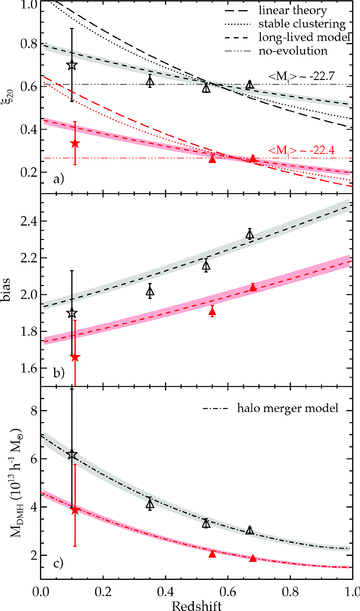
(a): The LRG ξ₂₀ measurements as a function of redshift and luminosity. The data at z≈ 0.1 (stars) are taken from the correlation functions of early-type galaxies in 2dFGRS (Norberg et al. 2002). Open and solid symbols correspond to the samples with median absolute magnitude, M_i− 5log₁₀h=−22.7 (SDSS/2SLAQ*/AAΩ*) and −22.4 (2SLAQ/AAΩ). The best fits for various models are also shown (see text for more details). The lower luminosity data have been lowered by 0.2 for clarity. (b) The LRG linear biases as a function of redshift and luminosity, comparing to the best-fitting long-lived model. (c) The typical mass of dark matter haloes occupied by the LRGs as estimated from the halo bias function. The dot–dashed lines are the best-fitting evolution model of dark matter halo mass via the merger framework (Lacey & Cole 1993).

Open in new tabDownload slide

Table 5

Open in new tab

Summary of the estimated LRG and 2dFGRS early-type galaxy bias factor and M_DMH as a function of redshift and luminosity.

Sample		−5log10h	b	MDMH (1013h−1 M⊙)
SDSS	0.35	−22.67	2.02 ± 0.04	4.1 ± 0.3
2SLAQ*	0.53	−22.69	2.16 ± 0.04	3.3 ± 0.2
AAΩ*	0.67	−22.60	2.33 ± 0.03	3.1 ± 0.1
2SLAQ	0.55	−22.40	1.91 ± 0.03	2.1 ± 0.1
AAΩ	0.68	−22.37	2.04 ± 0.02	1.9 ± 0.1
N02E1	≈0.1	−22.68	1.90 ± 0.23	6.2 ± 2.2
N02E2	≈0.1	−22.40	1.66 ± 0.20	3.9 ± 1.5

Sample		−5log10h	b	MDMH (1013h−1 M⊙)
SDSS	0.35	−22.67	2.02 ± 0.04	4.1 ± 0.3
2SLAQ*	0.53	−22.69	2.16 ± 0.04	3.3 ± 0.2
AAΩ*	0.67	−22.60	2.33 ± 0.03	3.1 ± 0.1
2SLAQ	0.55	−22.40	1.91 ± 0.03	2.1 ± 0.1
AAΩ	0.68	−22.37	2.04 ± 0.02	1.9 ± 0.1
N02E1	≈0.1	−22.68	1.90 ± 0.23	6.2 ± 2.2
N02E2	≈0.1	−22.40	1.66 ± 0.20	3.9 ± 1.5

Table 5

Open in new tab

Summary of the estimated LRG and 2dFGRS early-type galaxy bias factor and M_DMH as a function of redshift and luminosity.

Sample		−5log10h	b	MDMH (1013h−1 M⊙)
SDSS	0.35	−22.67	2.02 ± 0.04	4.1 ± 0.3
2SLAQ*	0.53	−22.69	2.16 ± 0.04	3.3 ± 0.2
AAΩ*	0.67	−22.60	2.33 ± 0.03	3.1 ± 0.1
2SLAQ	0.55	−22.40	1.91 ± 0.03	2.1 ± 0.1
AAΩ	0.68	−22.37	2.04 ± 0.02	1.9 ± 0.1
N02E1	≈0.1	−22.68	1.90 ± 0.23	6.2 ± 2.2
N02E2	≈0.1	−22.40	1.66 ± 0.20	3.9 ± 1.5

Sample		−5log10h	b	MDMH (1013h−1 M⊙)
SDSS	0.35	−22.67	2.02 ± 0.04	4.1 ± 0.3
2SLAQ*	0.53	−22.69	2.16 ± 0.04	3.3 ± 0.2
AAΩ*	0.67	−22.60	2.33 ± 0.03	3.1 ± 0.1
2SLAQ	0.55	−22.40	1.91 ± 0.03	2.1 ± 0.1
AAΩ	0.68	−22.37	2.04 ± 0.02	1.9 ± 0.1
N02E1	≈0.1	−22.68	1.90 ± 0.23	6.2 ± 2.2
N02E2	≈0.1	−22.40	1.66 ± 0.20	3.9 ± 1.5

To extend the redshift range, we shall compare our results to the clustering of early-type galaxies in 2dFGRS studied by Norberg et al. (2002) that roughly match the absolute magnitude of our samples after the K+e-correction. These are the samples with and ⁠, being compared to the SDSS/2SLAQ*/AAΩ* and 2SLAQ/AAΩ data and denoted as N02E1 and N02E2 in Table 5, respectively. We proceed in a similar fashion to the procedure described above and use the author’s best-fitting power law to estimate the ξ_{20, g}s and hence the bias values (see Table 5).

Both luminosity bins can be reasonably fitted by the long-lived model. The best-fitting models for the M_i− 5log₁₀h=−22.7 and −22.4 samples have b(0) = 1.93 ± 0.02 and 1.74 ± 0.02 with χ² = 7.34 [3 degrees of freedom (d.o.f.)] and 4.11 (2 d.o.f.), respectively, i.e. 1.5 − 1.9σ deviation. This is interesting given the lack of number density evolution seen in the LRG luminosity function by Wake et al. (2006). Nevertheless, it is intriguing that such a simple model gets so close to fitting data over the wide redshift range analysed here.

The stable model and the linear theory (with constant bias) model rise too quickly as the redshift decreases, excluded at >99.99 per cent confidence. However, the comoving model also gives a good fit to the SDSS/2SLAQ*/AAΩ* data in Fig. 14(a), as expected from the lack of evolution shown in Fig. 11(b). For this model to be exactly correct it would suggest that there was an inconsistency in these results with the underlying ΛCDM halo mass function. More certainly, we conclude that the evolution of the LRG clustering seems very slow. This general conclusion agrees with previous work (White et al. 2007; Wake et al. 2008). The latter author also only found a marginal rejection of the long-lived model from the large-scale clustering signal (1.8σ) compared to 1.9σ here. They found a much stronger rejection of a ‘passive’ evolution model from the small-scale LRG clustering and we shall return to this issue in Section 5.2.

5.1.2 LRG dark matter halo masses

The large-scale galaxy bias is roughly the same as that of the dark matter haloes which is a known function of mass threshold. Thus by measuring the clustering of the LRGs one can infer the typical mass of the haloes they reside in. The procedure employed here is similar to that used by Croom et al. (2005) and da Ângela et al. (2008) to estimate the dark matter halo masses of QSOs.

An ellipsoidal collapse model relating a halo bias factor to its mass was developed by Sheth et al. (2001) as an improvement over an earlier spherical collapse model of Mo & White (1996). In this analysis, we shall use the expression given in Sheth et al. (2001) and the revised parameters of Tinker et al. (2005) which were calibrated to give better fits to a wide range of σ₈ values for variants of ΛCDM model;

41

where a = 0.707, b = 0.35 and c = 0.80. ν is defined as ν=δ_c(z)/σ(M_DMH, z). δ_c is the critical density for collapse, and is given by δ_c = 0.15(12π)^2/3Ω_m(z)^0.0055 (Navarro et al. 1997). The rms fluctuation of the density field as a function of mass M_DMH at redshift z is σ(M_DMH, z) =σ(M_DMH)D(z) where σ(M_DMH) is given by

42

P(k) is the linear power spectrum of density perturbations and w(kr) is the window function, given by (Peebles 1980)

43

for a spherical top-hat function. The radius r can be related to mass via

44

where ρ₀=Ω⁰_mρ⁰_crit is the present mean density of the Universe, given by ρ₀ = 2.78 × 10¹¹Ω⁰_mh² M_⊙ Mpc⁻³. Here, we use the transfer function, T(k), fitting formula given by Eisenstein & Hu (1998) to construct P(k), assuming our fiducial cosmology (see Section 4.2).

The estimated dark matter halo masses of the LRG samples are given in Table 5 and plotted in Fig. 14(c). Note that the formalism of estimating dark matter halo masses from the galaxy biases used here assumes one galaxy per halo and can overestimate the threshold mass for a given value of bias (Zheng, Coil & Zehavi 2007). This is particularly true when we consider the mass estimated from equation (41) as the threshold mass, minimum mass required for a halo to host at least one galaxy and compare the results derived here to M_min from the best-fitting HOD (Section 4.3). However, if it is used as an estimate for the average mass of the host halo then it is underestimated by ≈40 per cent compared to the value given by the HOD due to the one galaxy per halo assumption.

Next, we attempt to fit the derived dark matter halo masses of these LRGs to the halo merger framework in hierarchical models of galaxy formation. We use the formalism discussed by Lacey & Cole (1993) to predict the median M_DMH of the descendants of virialized haloes at z = 1 for a given halo mass and fit this to our data. In essence, the model gives the probability distribution of the haloes with mass M₁ at time t₁ evolving into a halo of mass M₂ at time t₂ via merging. Fig. 14(c) shows the best-fitting models for the M_DMH evolution estimated in this way. These models appear to be good fits to both luminosity bins with the best-fitting M_DMH(z = 1) = 2.32 ± 0.07 × 10¹³h⁻¹ M_⊙ and 1.47 ± 0.05 × 10¹³h⁻¹ M_⊙ for the L≳ 3L* and ≳ 2L* samples, respectively.

The most massive haloes hosting these luminous early-type galaxies appear to have tripled their masses over the past 7 Gyr (i.e. half cosmic time) in stark contrast to the little evolution observed in the LRG stellar masses over the same period (see e.g. Wake et al. 2006; Cool et al. 2008). This lack of evolution contradicts the predictions in the standard hierarchical models of galaxy formation where one expects the most massive galaxies to form late via ‘dry’ merging of many less massive galaxies. However, this comes with a caveat that the M_DMH at z∼ 0 is an extrapolation [assuming Lacey & Cole (1993) halo merging model] of the z = 0.35–0.7 measurements and the constraint on the M_DMH(z = 0.1) is much weaker than the higher redshift results.

5.2 Small-scale clustering evolution

Finally, we discuss the evolution of the correlation function at scales corresponding to r < 1 h⁻¹ Mpc. We concentrate on comparing the number density matched AAΩ* and 2SLAQ* samples to the SDSS sample. As can be seen in Fig. 11(b), while at larger scales the w(θ) show amplitudes that are remarkably independent of redshift, at smaller scales the high redshift AAΩ* sample appears to have a lower amplitude than the lower redshift surveys. Here, we compare the clustering in non-linear regime to two clustering evolution models, namely stable clustering and HOD evolution models.

5.2.1 Stable clustering model

The stable model describes the clustering in the virialized regime and hence stable (unchanged) in proper coordinates (e.g. Phillipps et al. 1978). Therefore, assuming this model one expect the spatial correlation function to evolve as ξ(r)∝(1 +z)^{γ− 3}, where r is measured in comoving coordinates and γ is the power-law slope of the correlation function. Fig. 15 shows the small-scale, r≲ 1 h⁻¹ Mpc, w(θ) of the SDSS sample plus its best-fitting double power-law model, comparing to the evolved w(θ) from the z1 = 0.53 and 0.67 best-fitting models. Their ratios to the z = 0.35 best-fitting model are shown in the bottom panel with the shaded regions representing 1σ uncertainties in the best-fitting models. We see that the evolved z1 = 0.67 stable model underpredicts the z = 0.35 w(θ) somewhat but otherwise is within the 1σ regions of each other with the probability of acceptance P(<χ²) = 0.827. The agreement between the evolved z1 = 0.53 and the z = 0.35 is better, P(<χ²) = 0.999, given that the redshift difference is smaller. Note that the stable clustering model overpredicts the clustering amplitude at r≳ 1 h⁻¹ Mpc which is also observed in Fig. 14(a) as expected.

Figure 15

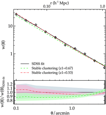
The small-scale w(θ) at z = 0.35 evolved from the best-fitting double power law of AAΩ* (green dashed line) and 2SLAQ* (red dot–dashed line) samples, assuming stable clustering model. The ratios of the evolved w(θ)s to the best-fitting double power law of SDSS sample are shown in the bottom panel. The shaded regions signify 1σ uncertainties in the best-fitting models.

Open in new tabDownload slide

The physical picture that is suggested is that the inflexion in the correlation function may represent the boundary between a virialized regime at small scales and a comoving or passively evolving biased regime at larger scales. As noted by Hamilton et al. (1991) and Peacock & Dodds (1996), the small-scale, non-linear, DM clustering is clearly expected from N-body simulations to follow the evolution of the virialized clustering model. However, for galaxies in a ΛCDM context, the picture may be more complicated.

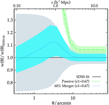
For example, by comparing the 2SLAQ and SDSS-LRG redshift surveys using the semi-projected correlation function, Wake et al. (2008) have suggested that a passively evolving model is rejected, weakly from the large-scale evolution but more strongly from the evolution at small scales. Wake et al. (2008) interpret the clustering evolution using an HOD description based on the ΛCDM halo mass function. Their ‘passive’ model predicts a far faster evolution at small scales than is given by our stable clustering (see Fig. 16). Our stable model is certainly passive in that it is based on the idea that the comoving number density of galaxies is independent of redshift. However, the passive HOD model of Wake et al. (2008) requires only 7.5 per cent of LRGs to merge between z = 0.55 and 0.19 to reconcile the slow LRG density and clustering evolution in the ΛCDM model. We shall see in the next section if this model can also accommodate our z = 0.68 clustering result while maintaining such a low merger rate.

Figure 16

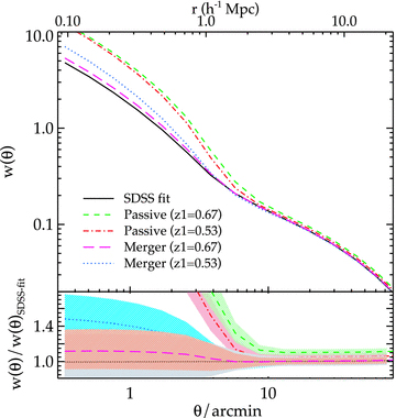
The predicted SDSS LRG w(θ) from passively (f_no-merge = 1) evolving the best-fitting HODs of 2SLAQ* (z1 = 0.53, red dot–dashed line) and AAΩ* (z1 = 0.67, green dashed line) samples. The results when central galaxies from high-redshift samples are allowed to merge (see text for more detail) are also shown, blue dotted and magenta long-dashed lines. The bottom panel shows the ratios of the evolved w(θ)s to the SDSS best fit, and the shaded regions signify the 1σ uncertainties.

Open in new tabDownload slide

5.2.2 HOD evolution

In Section 5.1.1, we found using the large-scale linear bias that the long-lived model (Fry 1996) is only marginally rejected at 1.5–1.9σ. This is in good agreement with the similar analysis of Wake et al. (2008). However, they argued that if the small-scale clustering signal was also taken into consideration, the long-lived model can be ruled out at much higher significance (>99.9 per cent).

Recall that our goodness of fit (based on the minimum χ²) for the halo models is rather poor (see Table 4). This may be an indication that a more complicated model may be needed, e.g. five-parameters HOD and/or a better two-halo-exclusion prescription, etc., given our small error bars. Nevertheless, the HOD fit generally describes the shape and amplitude of our measured w(θ) between 0.1 and 40 h⁻¹ Mpc. Therefore, at the risk of overinterpreting these HOD fits, we make a further test of the long-lived model by evolving the best-fitting HODs of the higher redshift samples to the SDSS-LRG average redshift.

Following the methods described in Wake et al. (2008, and references therein), the mean number of galaxies hosted by haloes of mass M at later time, z₀, is related to the mean number of galaxies in haloes of mass m, 〈N(m)〉, at earlier time, z₁, via

45

where N(m, M) is the conditional halo mass function of Sheth & Tormen (2002) which is the generalization of Lacey & Cole (1993) results, and C(M) and S(M) are the number of objects which used to be central and satellite galaxies.

We then model the central galaxy counts in the low-redshift haloes assuming that the progenitor counts in these haloes is ‘sub-Poisson’ (Sheth & Lemson 1999; Seo et al. 2008; Wake et al. 2008) such that

46

where N_max = int(M/M_min). This model is favoured by the Wake et al. (2008) analysis and is also seen in the numerical models of Seo et al. (2008). The mean number of satellite galaxies in the low-redshift haloes is then given by

47

where f_no-merge is the fraction of unmerged low-z satellite galaxies which were high-z central galaxies. This model is called ‘central–central mergers’ in Wake et al. (2008), where the more massive high-z central galaxies are more likely to merge with one another or the new central galaxy rather than satellite–satellite mergers.

For the long-lived model, we set f_no-merge = 1. The results of passively evolving the best-fitting HODs from z1 = 0.67 (AAΩ*) and z1 = 0.53 (2SLAQ*) to z0 = 0.35 are shown in Fig. 16 along with the SDSS best-fitting model. At large scales (r≥ 5 h⁻¹ Mpc), the long-lived model can only be marginally rejected at no more than 2σ for the AAΩ* case and is consistent within 1σ in the case of 2SLAQ*. However, if we now consider the small-scale, r < 1 h⁻¹ Mpc, clustering signal we see from the bottom panel of Fig. 16 that the long-lived model becomes increasingly inconsistent with the best-fitting model at z = 0.35. For r≥ 0.5 h⁻¹ Mpc, the long-lived model can be rejected at 99.88 and >99.99 per cent significance using the evolved 2SLAQ* and AAΩ* HODs, respectively. The much higher clustering signal at small scales is caused by far too many satellite galaxies in the low-redshift haloes being predicted by the long-lived model. This also results in the higher satellite fractions than observed; both evolved 2SLAQ* and AAΩ* give F_sat = 18 ± 1 per cent at z = 0.35 compared to 8.1 ± 1.8 seen in the SDSS best fit.

Next, we assume the central–central mergers model (Wake et al. 2008) and attempt to match the large-scale clustering signal of the evolved HOD from high-z to the z = 0.35 best-fitting model. As argued by Wake et al. (2008) and here, this is more likely to happen than the satellite–satellite merging case. The f_no-merge parameters in equation (47) required to give the best matches to the large-scale clustering amplitude of the SDSS best fit are 0.2 and 0.1 for the 2SLAQ* and AAΩ* case, respectively. The new w(θ)s determined from these models are plotted in Fig. 16 as the blue dotted and magenta long-dashed lines. We can see that the z1 = 0.67 evolved w(θ) at small scales is in excellent agreement with the SDSS best-fitting model. The predicted satellite fraction, F_sat = 7.8 ± 0.9, is also consistent with the SDSS best-fitting value. For the z1 = 0.53 case, the small-scale clustering signal is still somewhat stronger than the SDSS best-fitting model but otherwise are within 1σ confidence regions of each other, and the predicted F_sat = 10.5 ± 1.3 is also somewhat higher than the best-fitting value. The galaxy number density is reduced due to these central–central merger by ≈6 and 11 per cent for the z1 = 0.53 and 0.67, respectively. However, note that this is two to three times smaller than the fractional errors of our best-fitting n_g, ≈20 per cent.

In order to get a handle on the merger rates which can then be compared to the previous results of White et al. (2007) and Wake et al. (2008), we follow their method of adjusting the galaxy number density. This is because for this type of analysis the galaxy samples at different redshifts are usually designed to have the same space density. Merging means that the space density of the low-z sample must be reduced unless there are new galaxies created via merging of the fainter objects which fail to be in the high-z sample but become bright enough to be in the low-z sample. To account for such an effect by physically removing galaxies in a sample is rather difficult to do in practice as argued by Wake et al. (2008). White et al. (2007) and Wake et al. (2008) adjusted the mass-scale of the low-z HOD fit by several per cent which reduce the space density and increase the clustering signal and hence require lower amount of merging of the high-z population needed to match the low-z measurement. Increasing the f_no-merge factor in equation (47) results in a higher galaxy number density and clustering signal. Therefore, there is only one unique solution of mass-scaling and merging fraction that will simultaneously match the galaxy number density and the clustering signal (at large scales) of the evolved and best-fitting HODs at low z.

We increase the mass-scale of z = 0.35 HOD fit by 12 (7) per cent and allow 60 (50) per cent of the z1 = 0.67 (0.53) central galaxies to merge in order to get the matched large-scale bias of 2.12 (2.10) and n_g = 1.12(1.19) × 10⁻⁴h³ Mpc⁻³. This yields the merger rate between z = 0.67 (0.53) and z = 0.35 of ≈6.6 (5) per cent, i.e. ≈2.8 (3.4) per cent Gyr⁻¹. The evolved w(θ) divided by the model at z = 0.35 with increased mass-scaled HOD fit is shown in Fig. 17. As noted earlier, the reduction in the galaxy number density is small compared to its best-fitting fractional error which means that our constraints on these merger rates are rather weak. However, to the first order the merger rates derived here appear to be consistent with the value of 2.4 ± 0.7 and 3.4 per cent Gyr⁻¹ found by Wake et al. (2008) and White et al. (2007), respectively.

Figure 17

The ratio of the evolved w(θ) to the SDSS best-fitting model with the HOD mass-scale increased by 12 per cent.

Open in new tabDownload slide

In summary, the combination of the stable clustering and passive evolution model is remarkably close to explaining the clustering evolution of the LRGs at small and large scales. These models are much simpler than the HOD framework which require an understanding of how galaxies populate dark matter haloes and how they and their host haloes merge. The galaxy long-lived model in the context of halo framework is significantly incompatible with the small-scale clustering data and requires that ≈2–3 per cent/Gyr LRGs to merge in order to explain their slow clustering evolution. In contrast, the stable model requires the comoving number density to be constant with redshift. This may suggest that the simple virialized model may only provide a phenomenological fit to the small-scale clustering evolution in the context of the ΛCDM model.

6 SEARCHING FOR THE BAO PEAK

Next, we inspect the correlation functions at larger scales to make a search for the BAO feature. We first present the raw correlation functions in Fig. 18(a). Note that the integral constraints (see Section 3.1) are subdominant compared to w(θ)’s amplitudes at these scales. Each correlation function shows a feature at large scales, the most significant detection comes from the AAΩ sample where the clustering signal at 120 < θ < 500 arcmin is detected (above zero) at more than 4σ significance, P(<χ²) = 1 × 10⁻⁶ (with covariance matrix) and 3.5σ significance for 200 < θ < 500 arcmin.

Figure 18

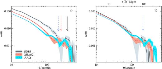
(a) The angular correlation function of the three LRG samples at large scales. The shaded regions are 1σ JK errors. The arrow indicates the expected BAO angular separation in each sample, assuming our fiducial cosmology. (b) Same as (a) but now scaled in the angular direction to the depth of the AAΩ-LRG sample.

Open in new tabDownload slide

The question is that are these features real or simply due to systematic error (see Section 6.1 for a series of systematic tests)? Here, we perform a classic scaling test to see if any feature is reproduced at the different depths of the three LRG samples. Given that the samples have intrinsically different r₀ (see Table 2), we choose simply to scale in the angular direction only. The SDSS and 2SLAQ LRG correlation functions are scaled in the angular direction to the AAΩ’s depth using the average radial comoving distance of each sample.

In Fig. 18(b), we see that the scaling agreement of the large-scale, θ≈ 300 arcmin, features is poor. Although SDSS shows a moderately strong peak feature, this is not reproduced at the same comoving physical scale in the other two data sets.

Despite this failure of the scaling test, we now attempt to increase the signal-to-noise ratio by combining the measurements from the three samples using inverse quadrature error weighting. First, the SDSS and 2SLAQ w(θ)s are scaled in the angular direction to the depth of the AAΩ LRGs (radial comoving distance, χ≈ 1737 h⁻¹ Mpc as opposed to ≈1451 h⁻¹ Mpc for 2SLAQ and ≈970 h⁻¹ Mpc for SDSS) where their amplitudes and errors are then interpolated to the AAΩ’s angular bins (i.e. Fig. 18b). The amplitudes of the scaled SDSS and 2SLAQ w(θ)s are then normalized to that of the AAΩ sample’s at 10 arcmin. This involves lowering SDSS and 2SLAQ amplitudes by 25 and 15 per cent, respectively. The resulting correlation function is presented in Fig. 19 with the arrow showing the expected position of the BAO peak. Note that due to the relatively small statistical errors of the AAΩ LRG compared to other samples, the w(θ) result is dominated by the AAΩ sample; therefore the possible SDSS peak at ≈100 h⁻¹ Mpc is not evident in the combined sample. There also seems to be an indication of an excess out to possibly 200 h⁻¹ Mpc (see Section 6.1 for a robustness test of this excess clustering signal).

Figure 19

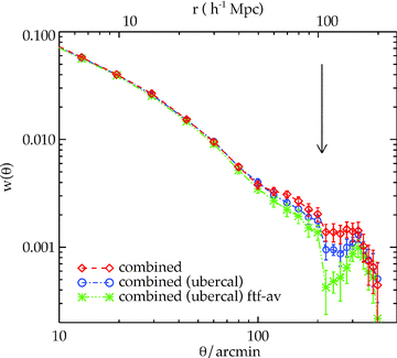
The combined angular correlation function of the three LRG samples scaled to the AAΩ depth, comparing the results when the SDSS standard (diamonds) and uber (circles) calibration are used. Also shown is the average field-to-field w(θ) (asterisks) which represents an attempt to filter out any large-scale gradients in the SDSS data.

Open in new tabDownload slide

Using the uber-calibration (Padmanabhan et al. 2008) instead of the standard calibration, we find similar results at small and intermediate scales but somewhat lower amplitude at ≈100 h⁻¹ Mpc although the results agree within the 1σ error (see Fig. 19). This means the correlation functions at small and intermediate scales including the parameters derived (e.g. power-law fits, linear biases, dark matter halo masses) in the earlier parts are not affected by which calibration we use. The biggest difference, although less than 1.5σ, is observed at scales larger than 120 h⁻¹ Mpc and up to 150 h⁻¹ Mpc where the correlation signal is small and hence more prone to possible systematics. The weak dependence of w(θ) at very large scales on the different calibrations may be an indication that this apparent extra peak at θ≈ 300 arcmin could indeed be a systematics effect. We shall return to this in Section 6.1.

We also tested whether the 200 h⁻¹ Mpc excess can be eliminated by taking the average w(θ) from 15 × 20 deg² subfields. The result, after integral constraint correction, is shown in Fig. 19. The 200 h⁻¹ Mpc excess persists even though there is some change at smaller scales. Given the model dependence introduced by the integral constraint correction (equation 11), hereafter we shall use the correlation function of the uber-cal sample measured using our normal method.

6.1 Testing for systematic effects

We have performed a series of tests to check our results against possible systematic effects. The tests include exclusions of high dust extinction and ‘poor’ astronomical seeing regions, an improved star–galaxy separation for the AAΩ sample and effects of possible contamination by clustered stars.

First, we exclude the regions where the i-band extinction is greater than 0.1 mag which discards ≈20 per cent of the data. The results are shown in the top row of Fig. 20. For 2SLAQ and AAΩ samples, the results appear to be lower than the main measurements but otherwise remain within 1σ statistical errors of each other. Although the amplitudes at θ≥ 220 arcmin are somewhat lower than the default AAΩ result, the excess at θ≳ 300 arcmin still persists. We then investigate the effect of excluding the regions with ‘poor’ astronomical seeing; the limit of 1.7 arcsec is used following the SDSS ‘poor’ seeing definition which discards ≈30 per cent of the data. The results here are in good agreement with the main results with the exception of a few angular bins around 320 arcmin of the 2SLAQ sample where they are somewhat (non-significantly) lower than the default measurements.

Figure 20

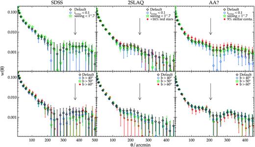
The angular correlation functions for SDSS, 2SLAQ and AAΩ samples (left to right), measured with varying dust extinction limit, astronomical seeing and different star–galaxy separation (top row), compared to our ‘Default’ results. Also shown is the effect of low galactic latitude region exclusion for each sample (bottom row). Note that for the b > 60°, the sample size is reduced by 60 per cent. In each case, an arrow indicates the expected position of the BAO peak assuming our fiducial cosmology.

Open in new tabDownload slide

Next, we attempt to reduce the stellar contamination fraction in the AAΩ sample. As a reminder, our default (optimized) star–galaxy separation algorithm (see Section 2) leaves ≈16 per cent stellar contamination in the sample while losing genuine LRGs only at a sub-per-cent level. Here, we impose a more aggressive star–galaxy separation cut which reduces the contamination level to ≈9 per cent at the expense of nearly halving the number of genuine AAΩ LRGs. The cut is a combination of the fitted ‘de Vaucouleurs’ radius as a function of z_deV magnitude and the correlation between the ‘de Vaucouleurs’ and fibre magnitudes in z band. The w(θ) measurement for this new AAΩ sample after correction by a factor of 1/(1 −f)², where f = 0.09, is shown in the top-right panel of Fig. 20. This is in good agreement with the main results.

We test our earlier assumption (Section 3; see also Blake et al. 2008) that the effect of the stellar contamination is simply a dilution of δ_g by (1 −f) and hence the amplitude of galaxy–galaxy correlation function by (1 −f)², where f is the contamination fraction. We add a sample of red stars to the 2SLAQ sample at the 16 per cent level, similar to what we expect in the AAΩ sample. The stars are selected from SDSS photometric objects which are classified as ‘star’. The colour selections have been matched to that of the AAΩ-LRG sample. The sample is then randomly selected to have the number of objects at 16 per cent of the 2SLAQ sample. They therefore follow the stellar distribution with galactic latitude. The w(θ) result after correction by 1/(1 −f)² is shown in the top-middle panel of Fig. 20 and is found to be in excellent agreement with the main 2SLAQ result. We do not see any evidence of a slope change which may arise from a possible clustering of the stellar contaminants at large scales, at least for the contamination level expected in our sample.

We apply various minimum galactic latitude cuts on the data in order to test for any systematic error. Such systematics (if they exist) could be due to the gradient caused by galactic dust extinction and/or different stellar contamination fractions which one might expect to be worse in the lower galactic latitude regions. Note that in our default data sets ≈95 per cent of the data are at b≥ 30°. The results of applying the galactic latitude cuts of b≥ 40°, 50° and 60° are shown in the bottom row of Fig. 20. Note that with the b≥ 60° limit, ≈60 per cent of the data are discarded. The 2SLAQ results appear to be marginally dependent on the galactic latitude limits. In the AAΩ sample the results are in good agreement with the main measurement although the b≥ 60° limit appears to be ≈1σ lower in some angular bins.

Finally, we cross-correlate the SDSS and AAΩ samples. The redshift distributions of the two samples are well separated with only slight overlap (see Fig. 1). Therefore, any residual signal in their cross-correlation function (CCF) at large scales can be used as evidence for systematic errors. The CCF is shown in Fig. 21, comparing to the auto-correlation functions of the SDSS and AAΩ samples in the top and bottom panels, respectively. The CCF has much lower signal than the auto-correlation function at θ < 120 arcmin and is consistent with zero, P(<χ²) = 0.997, between 120 < θ < 500 arcmin whereas the AAΩw(θ) signal is detected at more than 4σ significance (see above) in the same angular ranges.

Figure 21

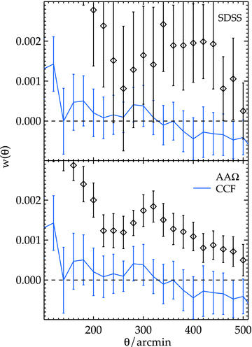
The auto-correlation functions for SDSS (top panel) and AAΩ (bottom panel) samples, comparing to the CCF between the two samples (blue solid lines).

Open in new tabDownload slide

We note that Ross et al. (2011) have suggested that there is a systematic effect associated with the area effectively masked by foreground stars which may be important in terms of a systematic that may produce excess clustering at large scales. However, such an effect would predict a decrease in galaxy density at low galactic latitudes and this is not seen in our samples (see fig. 9 of Sawangwit et al. 2010). If anything, the opposite effect is seen in our data with an increase in density towards lower galactic latitude which may be caused by stellar contamination. Here, we have tested our w(θ) measurements by successively cutting out data at low galactic latitudes. Although the 2SLAQ results may show some marginal dependence on the galactic latitude cut, the AAΩ results seem reasonably unaffected (see Fig. 20f). This may be due to the higher stellar contamination fraction in AAΩ sample which means that the effect seen by Ross et al. (2011) may not be directly applicable to the AAΩ sample.

We conclude that the apparent clustering excess at ≈300 arcmin in the AAΩ sample appears to be reasonably robust against most of the systematic tests we performed here. However, one might argue that the weakening of the excess signal when i_extinc > 0.1 regions (≈20 per cent) is excluded and the marginal dependence on the galactic latitude cuts of the 2SLAQ results may be taken as some evidence for systematic effects. On the other hand, the SDSS–AAΩ cross-correlation test also tends to limit the size of possible systematic errors.

6.2 Model comparisons

6.2.1 Standard ΛCDM model

First, we compare the measured angular correlation function to the perturbation theory prediction in the standard ΛCDM Universe. To compute the theoretical prediction, we proceed in the same manner as described in Section 4.2, calculating w(θ) by projecting ξ(r) which is a Fourier transform of a non-linear P(k). However, here we assume the best-fitting cosmological parameters from Eisenstein et al. (2005), a flat ΛCDM model with Ω_mh² = 0.13, Ω_bh² = 0.024, h = 0.7 and n = 0.98. Unlike in Section 4.2, the non-linear modelling of the BAO peak using only halofit is not adequate. The BAO peak in the correlation function can also be broadened (and perhaps slightly shifted) by the non-linear gravity suppression of the higher harmonics in the power spectrum via mode coupling (Meiksin, White & Peacock 1999). To model such an effect, we follow Eisenstein et al. (2005) and smoothly interpolate between the linear power spectrum and the ‘no-wiggle’ spectrum with the same overall shape but with the acoustic oscillations erased. This is done mathematically by

48

where P_lin is linear matter power spectrum, T_nw(k) and T_lin(k) are ‘no-wiggle’ and linear transfer functions computed from Eisenstein & Hu (1998) and x = exp (−k²a²) with a = 7 h⁻¹ Mpc chosen to fit the BAO suppression seen in their N-body simulations.

The P(k) is then corrected for non-linear gravitational collapse using the halofit software. The final P(k) is then transformed to ξ(r) using equation (19). Although the scale-dependent redshift-distortion and halo bias correction is weak at these scales, we follow Eisenstein et al. (2005) and multiply the correlation function by the square of 1 + 0.06/[1 + (0.06r)⁶] (solid line in their fig. 5), again chosen to fit what is seen in the N-body simulations. Such a correction is small at the BAO scale, only sub-per cent at r≳ 25 h⁻¹ Mpc and increases to ≈10 per cent at 10 h⁻¹ Mpc. We then correct for the linear redshift-space distortion; the ξ(s) amplitude is enhanced relative to the real-space correlation function, ξ(r), such that (Kaiser 1987)

49

Here, we assume β = 0.45 for these LRG samples (see Ross et al. 2007). The final ξ(s) model prediction with galaxy bias b = 2.09 for SDSS-LRG (see Section 4.2) is shown (cyan solid line) in the inset of Fig. 22. Eisenstein et al. (2005) find this model to be a good fit to their ξ(s) data with the best fit χ² = 16.1 on 17 d.o.f. for a particular set of cosmological parameters given above. We then computed w(θ) from the ξ(r) derived above via equation (14). Although the model (cyan solid line in Fig. 22) was found to be consistent with the LRG ξ(s), it is inconsistent with our w(θ) measurement, especially at r≳ 60 h⁻¹ Mpc or θ≳ 120 arcmin. The uber-cal AAΩw(θ) between 40 and 400 arcmin (corresponding to 20 ≲r≲ 200 h⁻¹ Mpc) are incompatible with the model at 99.8 per cent level (χ² = 39.3 over 18 − 1 d.o.f. with covariance matrix). We note that this rejection may be associated with the apparent clustering excess at θ≳ 200 arcmin, which still could be subject to systematics.

Figure 22

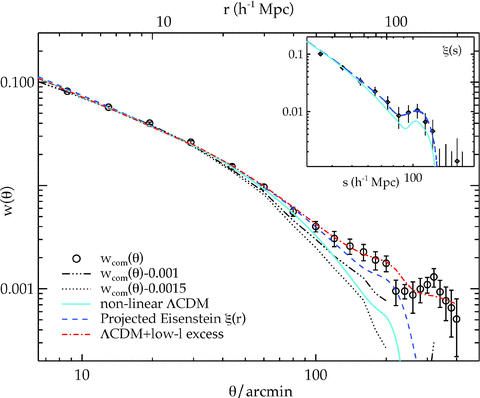
The combined w(θ) (open circles) compared to the projections of non-linear ΛCDM model plus mode coupling, scale-dependent redshift-space distortion and halo bias correction (cyan solid line) and the Eisenstein et al. (2005)ξ(s) (blue dashed line). The red dot–dashed line is the ΛCDM model plus low-l power excess (Section 6.2.2). The dash-dot–dotted and dotted lines show the effect of subtracting the data by 0.001 and 0.0015, respectively. The ξ(r) models used in the w(θ) projection are given as an inset together with the Eisenstein et al. (2005) measurement (diamonds). Here, the same symbols are used for the Eisenstein et al. (2005) and non-linear ΛCDM ξ(s) models as for the w(θ) models above.

Open in new tabDownload slide

Next, we compare our w(θ) to the best estimate of ξ(s) at the BAO scale as measured by Eisenstein et al. (2005). Although these measurements may have been superseded by DR7 spectroscopic LRG clustering analyses based on larger samples, these more recent estimates are usually in reasonable agreement with the results of Eisenstein et al. (2005), whether they are in correlation function (Martínez et al. 2009; Kazin et al. 2010) or power spectrum (Percival et al. 2010) form. For our comparison, we thus simply make a polynomial fit to the best estimate ξ(s) of Eisenstein et al. (2005) (blue dashed line in the inset of Fig. 22). The polynomial-fit ξ(s) is Kaiser de-boosted (equation 49) to give ξ(r) by assuming β = 0.45. The ξ(r) is then corrected for the linear growth between z = 0.35 and z = 0.68 which reduces the amplitude by ≈30 per cent. The resulting model has similar amplitude with the expected AAΩ-LRG ξ(r) because the SDSS and AAΩ-LRG linear biases are coincidentally the same (see Section 4.2). The model is then projected to w(θ) using equation (14) and is shown as a blue dashed line in Fig. 22. Our result appears to be in good agreement with the model up to ≈120 h⁻¹ Mpc given statistical uncertainties in our measurement and the ξ(s) data. Beyond ≈120 h⁻¹ Mpc, our w(θ) shows a higher clustering amplitude as noted above.

Summarizing, the w_com result appears consistent with the w(θ) prediction based on the Eisenstein et al. (2005) best estimate of ξ(s) (at least out to ≈120 h⁻¹ Mpc) but not with the prediction based on the flat ΛCDM model due to the apparent large-scale clustering excess in the w(θ). This means that given the size of error bars of the Eisenstein et al. (2005) result, the ΛCDM model is quite compatible with the ξ(s) data but given the much smaller statistical error on w(θ), in this case our measurements are inconsistent with the ΛCDM model. While the feature observed at ≈300 arcmin persists in most of the systematic tests we performed on the AAΩ samples (Section 6.1), a few of these tests, e.g. dust extinction, indicate there is still the possibility that systematic errors are affecting the w(θ). Therefore, if we now assume that the excess signal at ≈150 h⁻¹ Mpc is an indication of a systematic and subtract 0.001 to 0.0015, the level of the excess amplitude at this point in w_com (see Fig. 22), we obtain the w(θ) results as shown by the dash–dot-dotted and dotted lines. These two lines now bracket the flat ΛCDM result. Thus, the issue of the disagreement between the w(θ) result and the ΛCDM model seems to rest on the reality of the apparent clustering excess at large scales.

6.2.2 low-ℓ power excess?

Recently, Thomas, Abdalla & Lahav (2011a) (see also Padmanabhan et al. 2007; Blake et al. 2007; Thomas, Abdalla & Lahav 2011b) have also found a significant excess in their angular power spectrum, C_ℓ, at the low multipoles relative to the best-fitting ΛCDM models. They used photometric-redshift catalogues of the LRGs at z≈ 0.5 similar to our 2SLAQ sample. The most significant (≈4σ) low-ℓ power excess is observed in the highest redshift bin. The author carried out various systematic checks and found no indication of such an effect.

While the clustering excess only affects C_ℓ at multipoles smaller than the acoustic oscillations in Fourier space, unfortunately in configuration space the effect is expected on a wider range of scales and could affect our w(θ) BAO measurement.

Fig. 23 shows the Thomas et al. (2011a),C_ℓ and the excess power model used to predict the AAΩw(θ). For further detail of the low-ℓ power excess model, see Sawangwit (in preparation). The resulting w(θ) model with the amplitude normalized to fit the data at θ = 40–400 arcmin is shown as the red dot–dashed line in Fig. 22. The model appears to be consistent with our w_com (13 per cent confidence level, χ² = 23.6 over 18 − 1 d.o.f.) at r≈ 20–200 h⁻¹ Mpc. Therefore we note that the excess clustering signal in our w(θ) is in good agreement with that observed in the C_ℓ by Thomas et al. (2011a). The fact that the excess power in the C_ℓ has the form of an ℓ≈ 10 spike, suggests that this excess in w(θ) is due to something other than acoustic oscillations in the power spectrum.

Figure 23

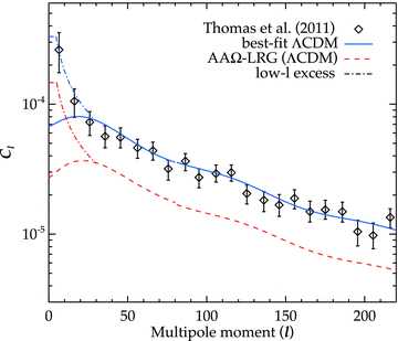
The angular power spectrum of the 0.6 < z < 0.65 MegaZ-DR7 LRG (Thomas et al. 2011b) with significant power excess at low multipoles (diamonds). The low-ℓ power excess plus the best-fitting ΛCDM model of the 0.6 < z < 0.65 C_ℓ (blue dot–dashed and solid lines) is extrapolated to the AAΩ redshift range (red dot–dashed and dashed lines).

Open in new tabDownload slide

We note that evidence for a large-scale (>150 h⁻¹ Mpc) correlation function excess has also been detected in the NRAO VLA Sky Survey (NVSS) radio source survey by Blake & Wall (2002) and Xia et al. (2010). We have compared our results with theirs and find that our correlation function shows a similar shape but a factor of 2–3 times lower amplitude. If the excess clustering signal observed here is real, then it could be evidence for non-Gaussianity (Xia et al. 2010) or for the gauge dependence of the matter power spectrum on the largest scales (Lin 2001; Yoo, Fitzpatrick & Zaldarriaga 2009). But until this feature is detected in an independent galaxy data set, there will always be the possibility that it is caused by some unknown systematics. Certainly, if the ΛCDM model were correct then we would have to conclude that this excess was caused by systematics at the level of Δw≈ 0.001–0.0015 in the photometric AAΩ-LRG sample.

7 SUMMARY AND CONCLUSIONS

We have presented here a new and detailed analysis of the angular correlation function of the LRGs extracted from the SDSS DR5 photometric catalogue. All the necessary information for inferring the spatial clustering is obtained and calibrated through redshift surveys of sample subsets. Our conclusions are as follows.

• We measured the angular correlation function of the LRGs at three different redshifts, namely 0.35, 0.55 and 0.68, and found the results to be well approximated by power laws at small and intermediate scales.

• With the large samples in terms of the numbers of objects and volume cover by the data, we see the deviation from the canonical single power law at high significance.

• The data are better fitted by a double power law where the large-scale (≳1–2 h⁻¹ Mpc) slope is equal to that of the conventional single power law, i.e. γ≈ 1.8.

• The form of the angular correlation functions at large scales is consistent with the expectation of the linear perturbation theory in the flat standard ΛCDM Universe.

• The LRG linear bias is high, b_g≈ 2.0, as expected for massive luminous early-type galaxies, and the clustering strength is found to be strongly linked to the sample intrinsic brightness.

• The best-fitting HOD models suggest that these LRGs reside in the massive dark matter haloes, 10¹³–10¹⁴h⁻¹ M_⊙, and are typically central galaxies in their dark matter halo hosts, with the satellite fraction no more than 10 per cent.

• The clustering evolution at intermediate scales (1 < r < 20 h⁻¹ Mpc) is remarkably slow and may be approximately explained by a long-lived model or even a no-evolution model. The long-lived model may be in line with the observed passive evolution of the LRG luminosity function, consistent with a constant comoving LRG space density in this redshift range. This latter conclusion would also apply in the case that the no-evolution (comoving) model were found to fit better but in this case the observations may require a significantly higher bias.

• Using the Lacey & Cole (1993) framework, our M_DMH(z) measurements are well fitted by the model where halo mass is grown via merging of progenitors with masses of ≈1.4 × 10¹³h⁻¹ M_⊙ and ≈2.3 × 10¹³h⁻¹ M_⊙ from z = 1, for haloes that typically host L≥ 2L* and ≥3L* galaxies, respectively. We found that these dark matter haloes have tripled their masses over the last half of cosmic time (although see the caveat given at the end of Section 5.1.2) whereas it has been claimed that the LRG stellar masses have grown by less than 50 per cent (Cool et al. 2008).

• At small scales (r < 1 h⁻¹ Mpc) the clustering evolution appears slightly faster at fixed luminosity and the clustering increases towards lower redshift, consistent with a virialized clustering model. Since our virialized model assumes a constant comoving LRG space density, a combination of this stable clustering model at small scales and the long-lived model at intermediate scales could be consistent with the idea that merging of LRGs may not change the LRG space density significantly out to z≈ 0.7.

• However, the evolution based on HOD and the ΛCDM halo merging framework requires that ∼ 2–3 per cent/Gyr of the LRGs merge with each other in order to explain the small-scale clustering evolution, consistent with the results of White et al. (2007) and Wake et al. (2008).

• In our AAΩ-LRG result we find a BAO peak at a level consistent with the best estimate of ξ(s) obtained by Eisenstein et al (2005). But, given the small size of our statistical errors, these results deviate significantly, ≈4σ, from the standard ΛCDM prediction because of an apparent large-scale clustering excess.

• The excess clustering signal generally persists after a series of systematic tests we performed. However, a few of these tests did change the feature somewhat, suggesting that it could still be caused by some unknown systematic effects.

• If the ΛCDM model were correct then we would have to conclude that this excess was caused by systematics at the level of Δw≈ 0.001–0.0015 in the photometric AAΩ-LRG sample.

• Otherwise, the excess signal in our w(θ) relative to the standard ΛCDM model appears to be in good agreement with the C_ℓ power excess at low l observed by other authors who used photo-z LRG samples at z≈ 0.5.

• If real, the large-scale clustering excess may be interpreted as evidence for a non-standard cosmological model, e.g. primordial non-Gaussianity or general relativistic effects. However, more, independent, data are required to check the reality of this clustering excess.

US acknowledges financial support from the Institute for the Promotion of Teaching Science and Technology (IPST) of The Royal Thai Government. We thank Michael J. I. Brown for useful comments. We thank the referee for useful comments which have improved the quality of the paper. We also thank all the present and former staff of the Anglo-Australian Observatory for their work in building and operating the 2dF and AAΩ facility.

Funding for the SDSS and SDSS-II has been provided by the Alfred P. Sloan Foundation, the Participating Institutions, the National Science Foundation, the US Department of Energy, the National Aeronautics and Space Administration, the Japanese Monbukagakusho, the Max Planck Society, and the Higher Education Funding Council for England. The SDSS Web Site is http://www.sdss.org/.

The SDSS is managed by the Astrophysical Research Consortium for the Participating Institutions. The Participating Institutions are the American Museum of Natural History, Astrophysical Institute Potsdam, University of Basel, Cambridge University, Case Western Reserve University, University of Chicago, Drexel University, Fermilab, the Institute for Advanced Study, the Japan Participation Group, Johns Hopkins University, the Joint Institute for Nuclear Astrophysics, the Kavli Institute for Particle Astrophysics and Cosmology, the Korean Scientist Group, the Chinese Academy of Sciences (LAMOST), Los Alamos National Laboratory, the Max-Planck-Institute for Astronomy (MPIA), the Max-Planck-Institute for Astrophysics (MPA), New Mexico State University, Ohio State University, University of Pittsburgh, University of Portsmouth, Princeton University, the United States Naval Observatory, and the University of Washington.

REFERENCES

Appendix

APPENDIX A: ANGULAR CORRELATION FUNCTIONS AND COVARIANCE MATRICES

At the referee’s request, we tabulate the angular correlation functions (Table A1) measured from the three photometric LRG samples studied in this paper. The full covariance matrices in the form of correlation coefficients are also shown in Fig. A1.