


Abstract
The aim of this paper is to present the results of photometric investigations of the central cluster of the W5 E H ii region as well as a follow-up study of the triggered star formation in and around bright-rimmed clouds (BRCs). We have carried out wide-field UBVIC and deep VIC photometry of the W5 E H ii region. A distance of ∼2.1 kpc and a mean age of ∼1.3 Myr have been obtained for the central cluster. The young stellar objects (YSOs) associated with the region are identified on the basis of near-infrared and mid-infrared observations. We confirmed our earlier results that the average age of the YSOs lying on/inside the rim is younger than those lying outside the rim. The global distribution of the YSOs shows an aligned distribution from the ionizing source to the BRCs. These facts indicate that a series of radiation-driven implosion processes proceeded from near the central ionizing source towards the periphery of the W5 E H ii region. We found that, in general, the age distributions of the Class II and Class III sources are the same. This result is apparently in contradiction to the conclusion by Bertout, Siess & Cabrit and Chauhan et al. that classical T Tauri stars evolve to weak-line T Tauri stars. The initial mass function of the central cluster region in the mass range 0.4 ≤M/M⊙≤ 30 can be represented by Γ=−1.29 ± 0.04. The cumulative mass functions indicate that in the mass range 0.2 ≤M/M⊙≤ 0.8, the cluster region and BRC NW have more low-mass YSOs compared to BRCs 13 and 14.
1 INTRODUCTION
Massive stars have a profound effect on the evolution of their natal molecular clouds. Their strong stellar winds and ultraviolet (UV) radiation cause an important feedback of energy and momentum in the surrounding medium. Once massive stars form they begin to ionize the remaining parental molecular cloud. The ionizing UV radiation has two competing effects on the parental molecular cloud. One is a negative feedback on the star formation activity, that is, the remaining molecular cloud is dispersed and further star formation is halted. The other is a positive feedback. The interaction can trigger new episodes of star formation as the H ii region expands into the molecular cloud. Two processes have been considered for the triggering of the star formation at the edge of the H ii region, namely ‘collect and collapse’ and ‘radiation-driven implosion (RDI)’. In the collect and collapse process, a compressed layer of high-density neutral material is accumulated between the ionization front (IF) and the shock front (SF). The dynamical instabilities in the compressed layer result in the fragmentation of the layer and formation of second-generation stars.
If the IF/SF encounters pre-existing denser parts, it compresses them to induce star formation. The process is known as RDI. Detailed model calculations of the RDI process have been carried out by several authors (e.g. Bertoldi 1989; Lefloch & Lazareff 1995; Kessel-Deynet & Burkert 2003; Miao et al. 2006). Star formation is predicted to occur in the initial short compression phase. This compression phase is followed by a transient phase of re-expansion and then by a quasi-stationary cometary phase. During the latter phase, the cloud represents a structure of a dense head and a long tail, and moves slowly away from the ionizing source by the rocket effect. The signature of the RDI process is the anisotropic density distribution of gas in a relatively small molecular cloud surrounded by a curved IF (bright rim) as well as a small group of young stellar objects (YSOs) in front of it.
Bright-rimmed clouds (BRCs) are small molecular clouds located near the edge of evolved H ii regions and show signs of the RDI and are hence considered to be good laboratories to study the physical processes involved in the RDI process. Sugitani, Tamura & Ogura (1995) carried out near-infrared (NIR) imaging of 44 BRCs and found that elongated small clusters or aggregates of YSOs, which are aligned towards the direction of the ionizing star, are often associated with them. These aggregates showed a tendency that ‘redder’ (presumably younger) stars tend to be located inside the BRCs, whereas relatively ‘bluer’ (presumably older) stars are found outside the clouds, suggesting an age gradient. Thus, they advocated a hypothesis called ‘small-scale sequential star formation (S4F)’. If the BRC is originally relatively large, the star formation may propagate along the axis of the BRCs as the IF/SF advances farther and farther into the molecular cloud (Kessel-Deynet & Burkert 2003).
The W5 H ii region is an extended H ii region with relatively simple morphology and shows indications of triggered star formation. It is a part of the large W3/W4/W5 cloud complex in the Perseus arm and consists of two adjacent circular H ii regions, W5 E and W5 W. There are many studies on this region. Karr & Martin (2003) discussed triggered star formation in W5 using multiwavelength archival data. Based on the time-scales of the expansion of the H ii region and the age of the YSOs, they obtained the time-scale of the interaction between the molecular clouds and the H ii region, t∼ 0.5–1.0 Myr. Using the Spitzer Space Telescope imaging with the Infrared Array Camera (IRAC) and Multiband Imaging Photometer for Spitzer (MIPS), Koenig et al. (2008) noted dense clusters of YSOs, centred around the O stars HD 17505, HD 17520, BD +60 586 and HD 18326. The H ii region W5 E is primarily ionized by HD 18326. Chauhan et al. (2009) (hereinafter Paper II) also paid attention to the cluster around this O7 V star. The W5 E H ii region has two BRCs, namely BRCs 13 and 14 (Sugitani, Fukui & Ogura 1991, hereinafter SFO 91) at its periphery. Based on the column densities of 13CO and the spatial distribution of YSO candidates, Niwa et al. (2009) identified a BRC candidate in the north-western part of the W5 E H ii region. We refer to this BRC candidate as BRC NW. Hence, W5 E is an interesting region to study triggered star formation.
In our earlier papers (Ogura et al. 2007, hereinafter Paper I; Paper II), we have studied the star formation scenario in/around six BRCs, including BRCs 13 and 14. The analysis was limited to the YSOs detected using the Hα emission and NIR excess only. A recent study by Koenig et al. (2008) has increased the number of YSOs in W5 E significantly. Hence, these data can be used to further investigate the YSO contents which we partly failed to detect in the Hα and NIR excess surveys reported in Paper I and Paper II.
In this paper, we have made an attempt to make photometric studies of the stellar content of the newly identified cluster in W5 E, by incorporating the NIR and mid-IR (MIR) data from the IRAC/MIPS of the Spitzer telescope. We have also considered the properties of the YSOs in the cluster as well as the three BRC regions to understand the star formation scenario in the W5 E H ii region. The influence of the ionizing source on the surrounding parental molecular cloud has also been discussed.
In Sections 2 and 3, we describe the observations, data reductions and archival data used in this work. Section 4 describes the analysis of the associated cluster. Sections 5 and 6 illustrate the procedure to estimate the membership, age, mass of the YSOs and total-to-selective extinction, RV, in the cluster and BRC regions. In Section 7, we discuss the initial mass function (IMF) and cumulative mass functions (CMFs) of the cluster and BRC regions. Section 8 describes the star formation scenario in the cluster and BRC regions. In Section 9, the disc evolution of T Tauri stars (TTSs) has been discussed.
2 OBSERVATIONS AND DATA REDUCTIONS
The 50×50 arcmin2 area containing the cluster around the O7 star HD 18326 that is noted by Koenig et al. (2008) and Chauhan et al. (2009) is reproduced from the DSS2-R image and shown in Fig. 1. As is evident from the figure, the cluster is embedded in an H ii region W5 E. BRCs 13 and 14 are located towards the eastern side, whereas BRC NW detected by Niwa et al. (2009) can be seen towards the north-west direction of the cluster. In the ensuing sections, we describe the observations carried out to study the region in detail.
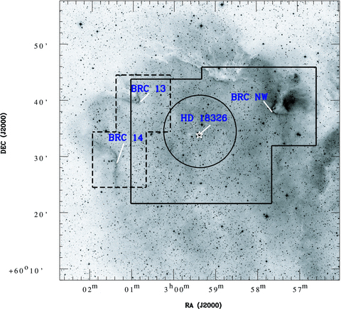
The 50 × 50-arcmin2 DSS2 R-band image of the W5 E H ii region. The area marked with the thick lines is the region for which deep images are taken in the V and IC bands. The dashed lines represent the boundaries of the region for which we have used data from our earlier work (Paper II). The circle represents the boundary of the cluster. The abscissa and the ordinate are RA and Dec for the J2000 epoch, respectively.
2.1 Optical CCD observations
The UBVIC CCD optical observations of W5 E were carried out using the the 2048 × 2048 pixel2 CCD camera mounted at the f/3.1 Schmidt focus of the 1.05-m telescope of the Kiso Observatory, Japan. The pixel size of 24 μm with an image scale of 1.5 arcsec pixel−1 covers a field of view of ∼50 × 50 arcmin2 on the sky. The average full width at half-maximum (FWHM) of the star images during the observations was ∼3 arcsec.
The UBVIC CCD observations of the central region of W5 E have also been carried out using the 2048 × 2048 pixel2 CCD camera mounted on the 1.04-m Sampurnanand Telescope (ST) of the Aryabhatta Research Institute of observational sciencES (ARIES), Nainital, India. To improve the signal-to-noise ratio (S/N), the observations were carried out in a binning mode of 2 × 2 pixel2. The pixel size is 24 μm with an image scale of 0.37 arcsec pixel−1 and the entire chip covers a field of ∼13 × 13 arcmin2 on the sky. The average FWHM of star images was ∼2.5 arcsec. The observations of the central region of W5 E were standardized on 2009 October 13 by observing standard stars in the SA 92 field (Landolt 1992). Deep imaging of a nearby field region towards the north from the cluster centre (α2000= ) was also carried out in the V and IC bands using the ST. The magnitudes of bright stars which were saturated in deep exposure frames have been taken from short exposure frames. A number of bias and twilight frames were also taken during the observing runs. The log of the observations is tabulated in Table 1.
Log of observations.
| α(2000) (hms) | δ(2000) ( ) ) | Filter: exposure (s) × number of frames | Date of observation (yyyy-mm-dd) |
| KISO | |||
| 02:59:22.60 | +60:33:48.7 | U: 180×9, 30×6; B: 60×9, 10×6; V: 60×9, 10×6; I: 60×9, 10×6 | 2007-10-20 |
| ST | |||
| 02:59:22.60 | +60:33:48.7 | U: 240×2, 10×1; B: 180×2, 5×1; V: 100×2, 4×1; I: 60×2, 4×1 | 2009-10-13 |
| 02:59:22.60 | +60:33:48.7 | U: 900×1, 300×1; B: 600×5; V: 360×9; I: 120×10 | 2006-12-16 |
| 03:00:08.34 | +60:39:19.3 | V: 600×5; I: 300×5 | 2007-10-13 |
| 02:58:38.78 | +60:39:06.1 | V: 600×5; I: 300×5 | 2007-10-13 |
| 03:00:03.49 | +60:27:59.6 | V: 600×5; I: 300×5 | 2007-10-13 |
| 02:58:33.34 | +60:28:47.2 | V: 300×10; I: 300×5 | 2007-11-06 |
| 02:57:44.41 | +60:38:29.1 | V: 180×2; I: 100×2 | 2009-10-13 |
| 02:57:44.41 | +60:38:29.1 | V: 600×6; I: 300×8 | 2009-10-15 |
| 02:59:34.13 | +61:05:28.4 | V: 300×10; I: 300×5 | 2006-12-15 |
| HCT | |||
| 02:59:23.83 | +60:34:00.0 | Gr7/167l: 300×1 | 2009-11-16 |
| α(2000) (hms) | δ(2000) () | Filter: exposure (s) × number of frames | Date of observation (yyyy-mm-dd) |
| KISO | |||
| 02:59:22.60 | +60:33:48.7 | U: 180×9, 30×6; B: 60×9, 10×6; V: 60×9, 10×6; I: 60×9, 10×6 | 2007-10-20 |
| ST | |||
| 02:59:22.60 | +60:33:48.7 | U: 240×2, 10×1; B: 180×2, 5×1; V: 100×2, 4×1; I: 60×2, 4×1 | 2009-10-13 |
| 02:59:22.60 | +60:33:48.7 | U: 900×1, 300×1; B: 600×5; V: 360×9; I: 120×10 | 2006-12-16 |
| 03:00:08.34 | +60:39:19.3 | V: 600×5; I: 300×5 | 2007-10-13 |
| 02:58:38.78 | +60:39:06.1 | V: 600×5; I: 300×5 | 2007-10-13 |
| 03:00:03.49 | +60:27:59.6 | V: 600×5; I: 300×5 | 2007-10-13 |
| 02:58:33.34 | +60:28:47.2 | V: 300×10; I: 300×5 | 2007-11-06 |
| 02:57:44.41 | +60:38:29.1 | V: 180×2; I: 100×2 | 2009-10-13 |
| 02:57:44.41 | +60:38:29.1 | V: 600×6; I: 300×8 | 2009-10-15 |
| 02:59:34.13 | +61:05:28.4 | V: 300×10; I: 300×5 | 2006-12-15 |
| HCT | |||
| 02:59:23.83 | +60:34:00.0 | Gr7/167l: 300×1 | 2009-11-16 |
Log of observations.
| α(2000) (hms) | δ(2000) () | Filter: exposure (s) × number of frames | Date of observation (yyyy-mm-dd) |
| KISO | |||
| 02:59:22.60 | +60:33:48.7 | U: 180×9, 30×6; B: 60×9, 10×6; V: 60×9, 10×6; I: 60×9, 10×6 | 2007-10-20 |
| ST | |||
| 02:59:22.60 | +60:33:48.7 | U: 240×2, 10×1; B: 180×2, 5×1; V: 100×2, 4×1; I: 60×2, 4×1 | 2009-10-13 |
| 02:59:22.60 | +60:33:48.7 | U: 900×1, 300×1; B: 600×5; V: 360×9; I: 120×10 | 2006-12-16 |
| 03:00:08.34 | +60:39:19.3 | V: 600×5; I: 300×5 | 2007-10-13 |
| 02:58:38.78 | +60:39:06.1 | V: 600×5; I: 300×5 | 2007-10-13 |
| 03:00:03.49 | +60:27:59.6 | V: 600×5; I: 300×5 | 2007-10-13 |
| 02:58:33.34 | +60:28:47.2 | V: 300×10; I: 300×5 | 2007-11-06 |
| 02:57:44.41 | +60:38:29.1 | V: 180×2; I: 100×2 | 2009-10-13 |
| 02:57:44.41 | +60:38:29.1 | V: 600×6; I: 300×8 | 2009-10-15 |
| 02:59:34.13 | +61:05:28.4 | V: 300×10; I: 300×5 | 2006-12-15 |
| HCT | |||
| 02:59:23.83 | +60:34:00.0 | Gr7/167l: 300×1 | 2009-11-16 |
The pre-processing of the data frames was done using the various tasks available under the iraf data reduction software package. The photometric measurements of the stars were performed using the daophot ii software package (Stetson 1987). The point spread function was obtained for each frame using several uncontaminated stars.
To study the luminosity function (LF)/mass function (MF) of the cluster region, we have used VIC data taken with the ST. It is necessary to take into account the incompleteness in the observed data that may occur for various reasons (e.g. crowding of the stars). A quantitative evaluation of the completeness of the photometric data with respect to the brightness and the position on a given frame is necessary to convert the observed LF to a true LF. We used the ADDSTAR routine of daophot ii to determine the completeness factor (CF). The procedure has been outlined in detail in our earlier works (see e.g. Pandey et al. 2001). We randomly added artificial stars to both V and IC images in such a way that they have similar geometrical locations but differ in IC brightness according to the mean (V−IC) colour (=1.5 mag) of the data sample. The luminosity distribution of artificial stars is chosen in such a way that more stars are inserted towards the fainter magnitude bins. The frames are reduced using the same procedure used for the original frame. The ratio of the number of stars recovered to that added in each magnitude interval gives the CF as a function of magnitude. The minimum value of the CF of the pair (i.e. V- and IC-band observations) for the two subregions, given in Table 2, is used to correct the data for incompleteness. The incompleteness of the data increases with increasing magnitude as expected. However, it does not depend on the area significantly.
Completeness factor of photometric data in the cluster and field regions.
| V range (mag) | Cluster region | Field region | |
| (r≤ 3′) | (3′ < r≤ 6′) | ||
| 13.5–14.0 | 1.00 | 1.00 | 1.00 |
| 14.0–14.5 | 1.00 | 1.00 | 1.00 |
| 14.5–15.0 | 0.99 | 0.99 | 1.00 |
| 15.0–15.5 | 0.98 | 0.98 | 0.99 |
| 15.5–16.0 | 0.98 | 0.98 | 0.98 |
| 16.0–16.5 | 0.96 | 0.97 | 0.98 |
| 16.5–17.0 | 0.97 | 0.96 | 0.98 |
| 17.0–17.5 | 0.97 | 0.96 | 0.98 |
| 17.5–18.0 | 0.95 | 0.95 | 0.96 |
| 18.0–18.5 | 0.93 | 0.94 | 0.95 |
| 18.5–19.0 | 0.91 | 0.92 | 0.94 |
| 19.0–19.5 | 0.88 | 0.90 | 0.91 |
| 19.5–20.0 | 0.85 | 0.84 | 0.89 |
| 20.0–20.5 | 0.81 | 0.82 | 0.84 |
| 20.5–21.0 | 0.72 | 0.71 | 0.77 |
| 21.0–21.5 | 0.51 | 0.54 | 0.57 |
The photometric results for the BRC 13 and BRC 14 regions have been taken from our earlier work (Paper II). They are based on observations with the Himalayan Faint Object Spectrograph Camera (HFOSC) on the 2.0-m Himalayan Chandra Telescope (HCT). The boundaries of the earlier observations are shown with the dashed lines in Fig. 1.
2.2 Grism slit spectroscopy
We obtained a low-resolution optical spectrum of the exciting star of W5 E, HD 18326, on 2009 November 16 using the HFOSC on the HCT, with a slit width of 2 arcsec and grism 7 (λ = 3800–6840Å, dispersion = 1.45 Å pixel−1). A one-dimensional spectrum was extracted from the bias-subtracted and flat-field-corrected image in the standard manner using iraf. The wavelength calibration of the spectrum was done using a FeAr lamp source. The standard star G191−B2B is used for the standardization and flux calibration.
3 ARCHIVAL DATA
3.1 NIR data from the Two-Micron All-Sky Survey
NIR JHKs data for point sources within a radius of 25 arcmin around the central cluster have been obtained from the Two-Micron All-Sky Survey (2MASS) Point Source Catalog (Cutri et al. 2003). Sources having uncertainty less than 0.1 mag (S/N ≥ 10) in all the three bands were selected to ensure high-quality data. The JHKs data were transformed from the 2MASS system to the California Institute of Technology (CIT) system using the relations given at the 2MASS website.1
3.2 MIR data from Spitzer
The NIR and MIR data (3.6–24 μm) from the Spitzer Space Telescope have provided the capability to detect and measure the IR excesses due to the circumstellar disc emission of the YSOs. In order to study the evolutionary stages of the YSOs detected using Spitzer, we used IRAC (3.6, 4.5, 5.8 and 8.0 μm) and MIPS (24 μm) photometry taken from Koenig et al. (2008).
3.3 Hα-emission stars from slit-less spectroscopy
The Hα-emission stars for the cluster region and BRC regions have been taken from Nakano et al. (2008) and Ogura, Sugitani & Pickles (2002), respectively.
4 ANALYSIS OF THE ASSOCIATED CLUSTER
4.1 Radial stellar surface density profile
The radial extent is one of the important parameters to study the dynamical properties of clusters. To estimate this, we assumed a spherically symmetric distribution of stars in the cluster. The star count technique is one of the useful tools to determine the distribution of cluster stars with respect to the surrounding stellar background.
In order to determine the cluster centre, we derived the highest peak of the stellar density by fitting a Gaussian profile to the star counts in strips along both the X-axis and the Y-axis around the eye estimated cluster centre. The cluster centre from the optical data has turned out to be at α2000= =
= . We repeated the same procedure using the 2MASS data to estimate the cluster centre and obtained it to be ∼12 arcsec away from the optical coordinates. However, this difference is within the uncertainty. Henceforth, we adopt the optical centre.
We estimated the radial density profile (RDP) to study the radial structure of the cluster. We divided the cluster into a number of concentric circles and the projected stellar density in each concentric annulus was obtained by dividing the number of stars by the respective annulus area. Stars brighter than V = 19.5 mag and K = 14.7 mag were considered for estimating the RDPs from the optical and 2MASS data, respectively. The densities thus obtained are plotted as a function of radius in Fig. 2. The error bars are derived assuming that the number of stars in each annulus follows the Poisson statistics.
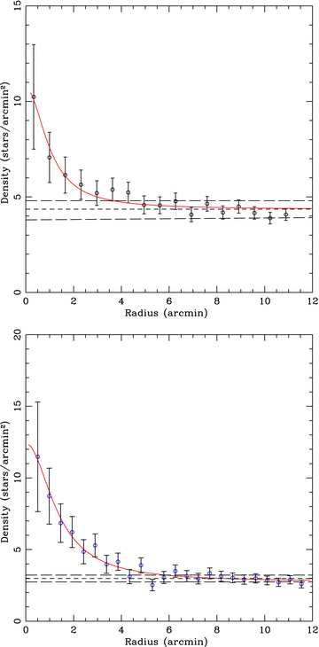
RDPs for the cluster using the optical (upper panel) and 2MASS (lower panel) data. The thick dashed line represents the mean density level of the field stars and the thin dashed lines are the error limits for the field star density. The continuous curve shows the least-squares fit of the King (1962) profile to the observed data points. The error bars represent  errors.
The extent of the cluster rcl is defined as the radius where the cluster stellar density merges with the field stellar density. The horizontal dashed line in the plot shows the field star density, which is obtained from a region ∼25 arcmin away towards the north from the cluster centre (α2000=02h 59m 34s; δ2000= ). Based on the RDP, we find that rcl is about 6 arcmin for stars brighter than V = 19.5 mag. Almost the same value for the cluster extent is obtained for the 2MASS data. We adopted a radius of 6 arcmin for this cluster to obtain the cluster parameters such as reddening, distance, IMF, etc.
4.2 Interstellar reddening
We know that the extinction or reddening E(B−V) of a star in a cluster arises due to two distinct sources:
the general interstellar medium (ISM) in the foreground of the cluster [E(B−V)f]; and
the localized ISM associated with the cluster [E(B−V)C=E(B−V) −E(B−V)f].
The former component is characterized by the ratio of the total-to-selective extinction RV [=AV/E(B−V)] = 3.1 (Wegner 1993; He et al. 1995; Winkler 1997), whereas, for the intracluster regions of young clusters embedded in a dust and gas cloud, the value of RV may vary significantly (Chini & Wargau 1990; Tapia et al. 1991; Pandey, Ogura & Sekiguchi 2000). The value of RV affects the distance determination significantly and consequently the age determination of stars. Several studies have already pointed out an anomalous reddening law with high RV values in the vicinity of star-forming regions (see e.g. Neckel & Chini 1981; Chini & Krüegel 1983; Chini & Wargau 1990; Pandey et al. 2000; Samal et al. 2007). Since the W5 E cluster and the BRCs are associated with the H ii region, it will be interesting to examine the reddening law in these objects. The ratio of the total-to-selective extinction RV is found to be normal in the cluster region (cf. Section 6 for details).
Since spectroscopic observations are not available, the interstellar reddening E(B−V) towards the cluster region is estimated using the (U−B)/(B−V) colour–colour (CC) diagram. The CC diagram of the cluster region is presented in Fig. 3. Since the cluster is very young, a variable reddening within the cluster region is expected. In Fig. 3, the continuous lines represent the intrinsic zero-age main sequence (ZAMS) by Girardi et al. (2002) which are shifted by E(B−V) = 0.62 and 0.80 mag along the normal reddening vector [i.e. E(U−B)/E(B−V) = 0.72] to match the distributions of probable cluster members. Fig. 3 thus yields a variable reddening with E(B−V)min = 0.62 mag to E(B−V)max = 0.80 mag in the cluster region. The stars lying within these two reddened ZAMSs may be probable members of the cluster. The reddening of individual stars with spectral classes earlier than A0 has been computed using the reddening-free index, Q (Johnson & Morgan 1953). Assuming a normal reddening law, we calculated Q = (U−B) − 0.72 × (B−V). The value of Q for stars earlier than A0 will be <0. For main-sequence (MS) stars, the intrinsic (B−V)0 colour and colour excess can be obtained by the relations (B−V)0 = 0.332 ×Q and E(B−V) = (B−V) − (B−V)0, respectively. Fig. 3 also indicates a large amount of contamination due to field stars. The probable late-type foreground stars with spectral types later than A0 may follow the ZAMS reddened by E(B−V) = 0.50 mag. A careful inspection of Fig. 3 indicates the presence of further reddened background populations. The reddening E(B−V) for the background population is found out to be in the range of ∼0.95–1.25 mag. This population may belong to the blue plume (BP) of the Norma–Cygnus arm (cf. Pandey, Sharma & Ogura 2006). The estimated E(B−V) values for the background population are comparable to the E(B−V) value of the BP population around l∼ 130° (cf. Pandey et al. 2006).

(U−B)/(B−V) CC diagram for the stars within the cluster radius (rcl≤ 6 arcmin). The continuous curves represent the ZAMS by Girardi et al. (2002) shifted along the reddening slope of 0.72 (shown as the dashed arrow) for E(B−V) = 0.62 and 0.80 mag, respectively. The dashed curves represent the ZAMS reddened by E(B−V) = 0.50, 0.95 and 1.25 mag, respectively, to match the probable foreground and background populations (see the text for details).
4.3 Spectral classification of the ionizing star in the W5 E H ii region
We obtained a slit spectrum of the brightest source to study its nature. In Fig. 4, we present the flux-calibrated, normalized spectrum of HD 18326, which is the ionizing source of the H ii region, in the wavelength range 3990–5000 Å. The important lines have been identified and labelled. HD 18326 is identified as an O7V- and O7V(n)-type star by Conti & Leep (1974) and Walborn (1973), respectively. The ratio of He iλ4471 to He iiλ4542 is a primary indicator of the spectral class of early-type stars. The ratio we found for this star is ∼1, which indicates that it is an O7 ± 0.5 star. With the present resolution of the spectrum, luminosity assessment is quite difficult. However, due to the presence of strong absorption in He iiλ4686, we assign the luminosity Class V.
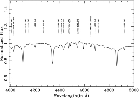
Flux-calibrated normalized spectrum of HD 18326.
4.4 Distance and optical colour–magnitude diagrams
The spectral class of the ionizing source yields an intrinsic distance modulus of 11.2 which corresponds to a distance of 1.74 kpc. Here, it is worthwhile noting that MV for an O7V star in the literature varies significantly, for example, MV=−5.2 (Schmidt-Kaler 1982) to −4.9 (Martins & Plez 2006). This star is also reported as a variable star and a suspected spectroscopic binary (Kazarovets, Durlevich & Samus 1998; Turner et al. 2008). Hence, the distance estimation based only on the O-type star alone may not be reliable. We also estimated the individual distance modulus of other probable MS stars. The intrinsic colours for each star were estimated using the Q method discussed in Section 4.2. We estimated corresponding MV values for each star using the ZAMS by Girardi et al. (2002). The average value of the intrinsic distance modulus, obtained using 24 probable MS members, comes out to be 11.65 ± 0.57, corresponding to a distance of 2.1 ± 0.3 kpc. This distance estimate is in agreement with those obtained by Becker & Fenkart (1971, 2.2 kpc), Georgelin & Georgelin (1976, 2.0 kpc) and Hillwig et al. (2006, 1.9 kpc).
We used the optical colour–magnitude diagrams (CMDs) to derive the fundamental parameters of the cluster, such as age, distance, etc. The V/(B−V) and V/(V−I) CMDs for stars lying within the 6 arcmin radius are shown in Figs 5(a) and (b). Fig. 5(c) shows the V/(V−I) CMD for a nearby field region (see Section 4.1). A 4-Myr isochrone for Z = 0.019 by Girardi et al. (2002) and the pre-MS (PMS) isochrones for 1 and 5 Myr by Siess, Dufour & Forestini (2000) have also been plotted for (m−MV) = 13.5 mag and E(B−V) = 0.62 mag, assuming E(V−I) = 1.25 × E(B−V) and RV = 3.1. A comparison of the CMDs of the cluster region with that of the field region reveals an unambiguous population of PMS sources along with a significant contamination due to the field star population.
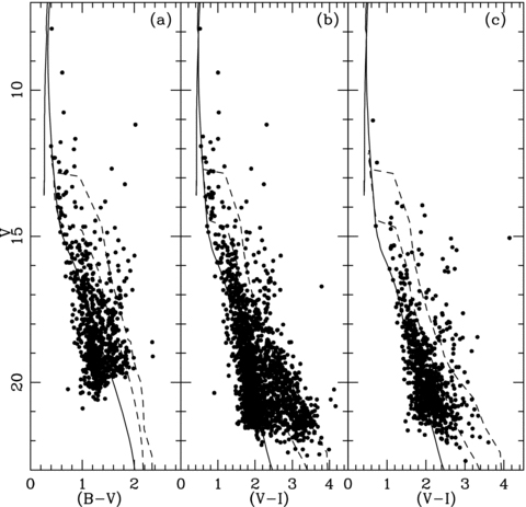
Panels (a) and (b): the V/(B−V) and V/(V−I) CMDs for the stars within the cluster radius; panel (c): the V/(V−I) CMD for stars in the field region having the same area as in panels (a) and (b). The continuous line is the isochrone of 4 Myr from Girardi et al. (2002) and the dashed lines are 1- and 5-Myr PMS isochrones from Siess et al. (2000). The isochrones are corrected for the cluster distance of 2.1 kpc and reddening E(B−V) = 0.62 mag.
5 IDENTIFICATION OF PMS OBJECTS ASSOCIATED WITH THE CLUSTER AND BRCs
Since the W5 E H ii region is located at a low Galactic latitude, the region is significantly contaminated by foreground/background stars as discussed above. In order to understand the star formation in the region, we selected probable PMS members associated with the region using the following criteria.
Some PMS stars, specifically classical TTSs (CTTSs), show emission lines in their spectra, among which usually Hα is the strongest. Therefore, Hα-emission stars can be considered as good candidates for PMS stars associated with the region. In this study, we use Hα-emission stars found by Ogura et al. (2002) and Nakano et al. (2008) in the W5 E H ii region. Since many PMS stars also show NIR/MIR excesses caused by circumstellar discs, NIR/MIR photometric surveys are also powerful tools to detect low-mass PMS stars. We have also used the YSOs identified by Koenig et al. (2008) in the W5 E H ii region using Spitzer IRAC and MIPS photometry.
Fig. 6(a) shows the NIR (J−H)/(H−K) CC (NIR-CC) diagram of all the sources detected in the 2MASS catalogue along with the YSOs identified by Koenig et al. (2008) in the cluster region, whereas Fig. 6(b) shows the NIR-CC diagram for the sources in the nearby reference field. In Figs 6(a) and (b), the thin and long-dashed curves represent the unreddened MS and giant branches (Bessell & Brett 1988), respectively. The dotted line indicates the locus of intrinsic CTTSs (Meyer, Calvet & Hillenbrand 1997). The curves are also in the CIT system. The parallel dashed lines are the reddening vectors drawn from the tip (spectral type M4) of the giant branch (‘upper reddening line’), from the base (spectral type A0) of the MS branch (‘middle reddening line’) and from the tip of the intrinsic CTTS line (‘lower reddening line’). The extinction ratios AJ/AV = 0.265, AH/AV = 0.155 and AK/AV = 0.090 have been adopted from Cohen et al. (1981). We classified sources into three regions in the NIR-CC diagrams (cf. Ojha et al. 2004a). ‘F’ sources are located between the upper and middle reddening lines and are considered to be either field stars (MS stars, giants) or Class III sources and Class II sources with small NIR excesses. ‘T’ sources are located between the middle and lower reddening lines. These sources are considered to be mostly CTTSs (Class II objects). There may be an overlap in NIR colours of Herbig Ae/Be stars and CTTSs in the ‘T’ region (Hillenbrand et al. 1992). ‘P’ sources are those located in the region redwards of the ‘T’ region and are most likely Class I objects (protostar-like objects; Ojha et al. 2004b). So, objects falling in the ‘T’ and ‘P’ regions of NIR-CC diagrams are considered to be NIR-excess stars and hence are probable members of the cluster. These sources are included in the analysis of this study in addition to Hα-emission stars. It is worthwhile, however, to note that Robitaille et al. (2006) have recently shown that there is a significant overlap between protostars and CTTSs in the NIR-CC space.
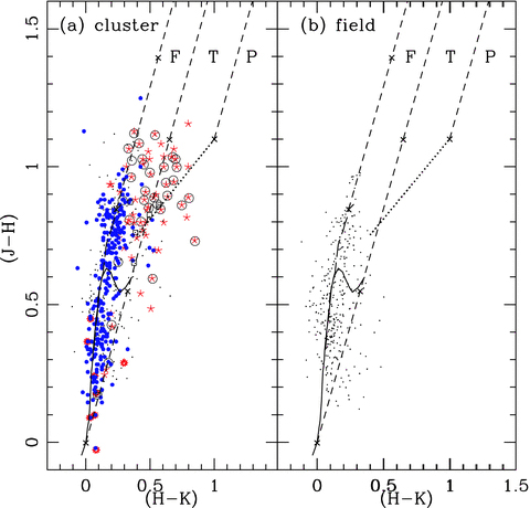
NIR (J−H)/(H−K) CC diagrams for the stars (a) within the cluster radius and (b) in the reference field. The small dots represent 2MASS sources and the open circles represent Hα sources from Nakano et al. (2008). Class II, Class III and transition sources from Spitzer photometry are shown by the asterisks, filled circles and open squares, respectively. The dashed straight lines represent the reddening vectors (Cohen et al. 1981). The crosses on the dashed lines are separated by AV = 5 mag.
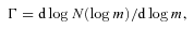
The V/(V−I) CMD for the YSOs taken from the catalogue by Koenig et al. (2008) for the cluster region (rcl = 6 arcmin) is shown in Fig. 7. Here the well-known age-with-mass trend that higher mass stars look older than lower mass stars (Hillenbrand, Bauermeister & White 2008) is evident. In addition, a few sources, having V≳ 15, classified as Class III objects are located near the MS. They are also located on the MS in the NIR-CC diagram and hence could be field stars. This indicates that part of Class III objects by Koenig et al. (2008) are not YSOs, but rather stars found in the W5 Spitzer photometric sample that appear to have photospheric colours in the 3–24 μm bands and thus appear as Class III SEDs. Thus, the listed Class III objects by Koenig et al. (2008) may be heavily contaminated by foreground and background field populations. A comparison of the NIR-CC diagram of the cluster region and nearby field region indicates that the YSOs identified by Koenig et al. (2008) and having (J−H) > 0.7 mag and (H−K) > 0.3 mag can be safely considered as YSOs associated with the region.
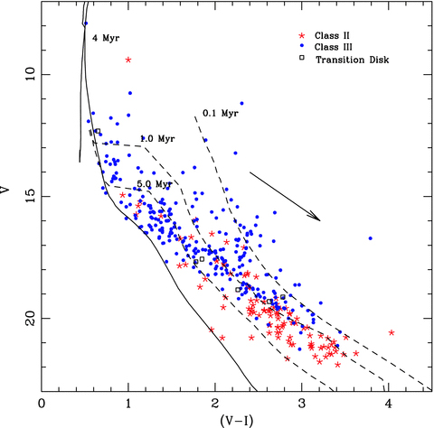
V/(V−I) CMD for the clustered YSOs identified by Koenig et al. (2008) in the cluster region. The continuous line is the isochrone of 4 Myr from Girardi et al. (2002) and the dashed lines are the 0.1-, 1- and 5-Myr PMS isochrones from Siess et al. (2000). The isochrones are corrected for the cluster distance of 2.1 kpc and reddening E(B−V) = 0.62 mag.
The NIR-CC diagrams for the identified YSOs (with Hα emission and IR excess) in BRC NW, BRC 13 and BRC 14 are shown in Figs 8(a), (b) and (c), respectively. The NIR-CC diagrams were used to estimate AV for each of these YSOs by tracing them back to the intrinsic CTTS locus of Meyer et al. (1997) along the reddening vector (for details see Paper I and Paper II). The AV for the stars lying in the ‘F’ region is estimated by tracing them back to the extension of the intrinsic CTTS locus. The mean reddening for each BRC region is calculated. The mean AV values for BRC NW, BRC 13 and BRC 14 are found to be 2.26, 2.33 and 3.05 mag, respectively. Fig. 9 shows the V/(V−I) CMDs of the YSOs selected using the NIR-CC diagram in the cluster region as well as in the three BRC regions. Again, the CMDs indicate that practically all of them are PMS stars but, at the same time reveal a significant scatter in their age. The age of each YSO was estimated by referring to the isochrones. The mass of the YSOs was estimated using the V/(V−IC) CMD as discussed in Pandey et al. (2008) and Chauhan et al. (2009). The resultant age and mass are given in Table 3, the full version of which is available with the electronic version of this paper (see Supporting Information). Here, we would like to point out that the estimation of the age of the PMS stars by comparing the observations with the theoretical isochrones is prone to two kinds of errors: random errors in observations and systematic errors due to the variation between the predictions of different theoretical evolutionary tracks (see e.g. Hillenbrand 2005; Hillenbrand et al. 2008). The effect of random errors in the determination of the age and mass was estimated by propagating the random errors to their observed estimation by assuming a normal error distribution and using Monte Carlo simulations. The use of different PMS evolutionary models gives different ages and hence an age spread in a cluster (e.g. Sung, Chun & Bessel 2000). In this study, we have used the models by Siess et al. (2000) only for all the BRCs and the cluster region; therefore, our age and mass estimations are not affected by the systematic errors. However, the use of different sets of PMS evolutionary tracks will introduce a systematic shift in the age determination. The presence of binaries may be another source of errors in the age determination. Binarity will brighten the star; consequently, the CMD will yield a lower age estimate. In the case of equal-mass binaries, we expect an error of ∼50–60 per cent in the age estimation of the PMS stars. However, it is difficult to estimate the influence of binarity on the mean age estimation as the fraction of binaries is not known.
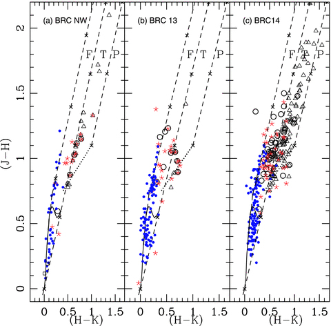
The (J−H)/(H−K) CC diagrams of the YSOs in BRC NW, BRC 13 and BRC 14. Class I, Class II, Class III and transition sources from Spitzer photometry are shown by the filled triangles, asterisks, filled circles and open squares, respectively. NIR-excess sources from the 2MASS and Matsuyanagi et al. (2006) (in case of BRC 14) are shown by the open triangles and Hα sources from Ogura et al. (2002) are shown by the open circles.

V/(V−I) CMDs for the YSOs selected in this study (see the text) in the (a) cluster, (b) BRC NW, (c) BRC 13 and (d) BRC 14 regions. The continuous line is the isochrone of 4 Myr from Girardi et al. (2002) and the dashed lines are 0.1-, 1- and 5-Myr PMS isochrones from Siess et al. (2000). The isochrones are corrected for the distance and reddening of the respective regions. The arrow represents the reddening vector.
The B, V and IC photometric data along with their position, mass and age for the YSOs in the cluster and BRC regions. This is a sample of the full table, which is available with the electronic version of the paper (see Supporting Information).
| S. No. | α2000 (hms) | δ2000 ) ) | B±eB (mag) | V±eV (mag) | I±eI (mag) | Age ±σ (Myr) | Mass ±σ (M⊙) |
| Cluster region | |||||||
| 1 | 02:58:39.03 | 60:37:25.8 | – | 19.67 ± 0.02 | 16.78 ± 0.02 | 0.3 ± 0.01 | 0.38 ± 0.00 |
| 2 | 02:58:39.24 | 60:37:02.7 | 20.07 ± 0.02 | 18.21 ± 0.01 | 15.60 ± 0.01 | 0.15 ± 0.02 | 0.52 ± 0.00 |
| 3 | 02:58:39.32 | 60:35:00.6 | – | 20.78 ± 0.03 | 18.05 ± 0.02 | 2.39 ± 0.05 | 0.44 ± 0.01 |
| – | ––– | ––– | –— | ––– | ––– | –– | –– |
| – | ––– | ––– | –— | ––– | ––– | –– | –– |
| S. No. | α2000 (hms) | δ2000) | B±eB (mag) | V±eV (mag) | I±eI (mag) | Age ±σ (Myr) | Mass ±σ (M⊙) |
| Cluster region | |||||||
| 1 | 02:58:39.03 | 60:37:25.8 | – | 19.67 ± 0.02 | 16.78 ± 0.02 | 0.3 ± 0.01 | 0.38 ± 0.00 |
| 2 | 02:58:39.24 | 60:37:02.7 | 20.07 ± 0.02 | 18.21 ± 0.01 | 15.60 ± 0.01 | 0.15 ± 0.02 | 0.52 ± 0.00 |
| 3 | 02:58:39.32 | 60:35:00.6 | – | 20.78 ± 0.03 | 18.05 ± 0.02 | 2.39 ± 0.05 | 0.44 ± 0.01 |
| – | ––– | ––– | –— | ––– | ––– | –– | –– |
| – | ––– | ––– | –— | ––– | ––– | –– | –– |
The B, V and IC photometric data along with their position, mass and age for the YSOs in the cluster and BRC regions. This is a sample of the full table, which is available with the electronic version of the paper (see Supporting Information).
| S. No. | α2000 (hms) | δ2000) | B±eB (mag) | V±eV (mag) | I±eI (mag) | Age ±σ (Myr) | Mass ±σ (M⊙) |
| Cluster region | |||||||
| 1 | 02:58:39.03 | 60:37:25.8 | – | 19.67 ± 0.02 | 16.78 ± 0.02 | 0.3 ± 0.01 | 0.38 ± 0.00 |
| 2 | 02:58:39.24 | 60:37:02.7 | 20.07 ± 0.02 | 18.21 ± 0.01 | 15.60 ± 0.01 | 0.15 ± 0.02 | 0.52 ± 0.00 |
| 3 | 02:58:39.32 | 60:35:00.6 | – | 20.78 ± 0.03 | 18.05 ± 0.02 | 2.39 ± 0.05 | 0.44 ± 0.01 |
| – | ––– | ––– | –— | ––– | ––– | –– | –– |
| – | ––– | ––– | –— | ––– | ––– | –– | –– |
6 REDDENING LAW IN THE CLUSTER AND BRC REGIONS
To study the nature of the extinction law in the region, we used two-colour diagrams (TCDs) as described by Pandey et al. (2003). The TCDs of the form of (V−λ) versus (B−V), where λ is one of the broad-band filters (R, I, J, H, K, L), provide an effective method of separating the influence of the normal extinction produced by the diffuse ISM from that of the abnormal extinction arising within regions having a peculiar distribution of dust sizes (cf. Chini & Wargau 1990; Pandey et al. 2000).
The TCDs for the Class III YSOs associated with the cluster and BRC regions are shown in Figs 10(a)–(d). In order to avoid IR-excess stars, we have used all the Spitzer Class III sources having V < 17 mag. The slopes of the distributions are given in the figure. The ratio of the total-to-selective extinction ‘RV’ in the regions is estimated using the procedure described in Pandey et al. (2003). The RV values in the cluster and BRC regions, that is, BRC NW, BRC 13 and BRC 14, are estimated to be Rcluster = 3.14 ± 0.12, RBRC NW = 3.46 ± 0.20, RBRC 13 = 3.41 ± 0.03 and RBRC 14 = 2.75 ± 0.12, respectively. The value of Rcluster indicates a normal reddening law in the cluster region. The higher values of RBRC NW and RBRC 13 indicate a larger grain size in the BRC NW and BRC 13 regions, whereas the smaller value of RBRC 14 suggests a smaller grain size in the case of BRC 14. This indicates that the evolution of dust grains in the W5 E region has not taken place in a homogeneous way.
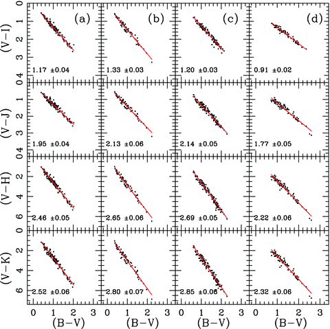
TCDs for the disc-less (Class III) sources in the (a) cluster, (b) BRC NW, (c) BRC 13 and (d) BRC 14 regions.
7 MASS FUNCTIONS OF THE CLUSTER AND BRC REGIONS
7.1 IMF of the cluster
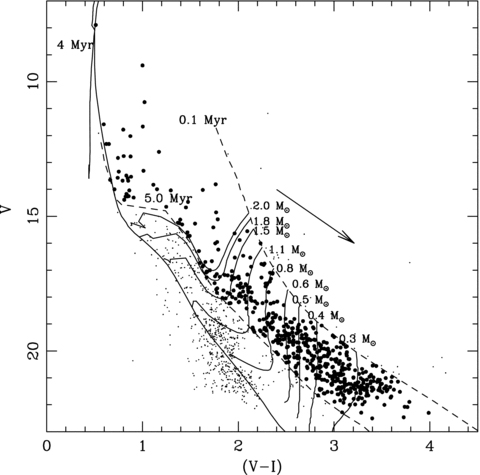
To study the MF and LF, it is necessary to eliminate the field star contamination from the cluster region. In the absence of proper motion data, one can use statistical criteria to estimate the number of probable member stars in the cluster region. To remove the contamination due to field stars from the MS and PMS samples, we statistically subtracted the contribution of field stars from the observed CMD of the cluster region using the following procedure. For any star in the V/(V−I) CMD of the control field (Fig. 5c), the nearest star in the cluster's V/(V−I) CMD (Fig. 5b) within V± 0.125 and (V−I) ± 0.065 was removed. The statistically cleaned CMD is shown in Fig. 11, which clearly shows a sequence of PMS stars. The PMS isochrones by Siess et al. (2000) for the ages of 0.1 and 5 Myr (dashed lines) and the 4-Myr isochrone by Girardi et al. (2002) (continuous line) are shown in Fig. 11. The evolutionary tracks by Siess et al. (2000) for different masses are also shown which are used to estimate the mass of PMS stars. Here we would like to note that the points shown by the filled circles in Fig. 11 may not represent the actual members of the clusters. However, the filled circles should represent the statistics of PMS stars that can be used to study the MF of the cluster region. We used the statistics of the sources having an 0.1 ≤ age ≤ 5 Myr in the statistically cleaned CMD (Fig. 11) to study the IMF of the cluster region. It is also important to make corrections in the data sample for incompleteness which may be due to various reasons, for example, crowding of the stars. We determined the CF as described in Section 2.1. Since the MS age of the most massive star in the cluster is <4 Myr, the stars having V < 14.7 mag (M > 3 M⊙) have been considered on the MS. In order to obtain the MF for MS stars, the LF is converted to the MF using the theoretical model of Girardi et al. (2002). The MF of the PMS stars was obtained by counting the number of stars in different mass bins (for details see Pandey et al. 2008; Jose et al. 2008). Fig. 12 shows the MF of the cluster in the mass range 0.4 ≤M/M⊙≤ 30. A single slope for the MF in the mass range 0.4 ≤M/M⊙≤ 30 can be fitted with Γ=−1.29 ± 0.04, which is comparable to the Salpeter value (−1.35).
Statistically cleaned V/(V−I) CMD for stars lying within the cluster radius. The stars having the PMS age ≤ 5 Myr are considered as representing the statistics of PMS stars in the region and are shown by the filled circles. The 4-Myr isochrone by Girardi et al. (2002), and the 0.1- and 5.0-Myr PMS isochrones along with evolutionary tracks for different masses by Siess et al. (2000) are also shown. All the isochrones are corrected for the cluster distance and reddening. The corresponding values of masses in solar mass are given at the right-hand side of each track. The points shown by the small dots are considered as non-members. The arrow represents the reddening vector.
The MF in the cluster region derived using the optical data. φ represents N/d log m. The error bars represent  errors. The continuous line shows the least-squares fit to the mass ranges described in the text. The value of the slope obtained is mentioned in the figure.
7.2 Cummulative MF of identified YSOs in the cluster and BRC regions
The MF is an important tool to compare star formation processes/scenarios in different regions. Morgan et al. (2008), based on SCUBA observations, have estimated the mass of 47 dense cores within the heads of 44 BRCs. They concluded that the slope of the MF of these cores is significantly shallower than that of the Salpeter MF. They also concluded that it depends on the morphological type of BRCs (for the morphological description of BRCs, refer to SFO 91): ‘A’-type BRCs appear to follow the mass spectrum of the clumps in the Orion B molecular cloud, whereas the BRCs of the ‘B’ and ‘C’ types have a significantly shallower MF.
In Paper II, we have studied the CMFs of YSOs selected on the basis of NIR excess and Hα emission and found that the ‘A’-type BRCs seem to follow a MF similar to that found in young open clusters, whereas ‘B/C’-type BRCs have a significantly steeper CMF, indicating that BRCs of the latter type tend to form relatively low mass YSOs in the mass range 0.2 ≤M/M⊙≤ 0.8. The CMF of the YSOs associated with the ‘A’-type BRCs in the mass range 0.2 ≤M/M⊙≤ 0.8 is found to be comparable with the CMF of the average Galactic IMF (cf. Paper II).
As mentioned above, in Paper II, the YSOs were selected on the basis of NIR excess and Hα emission. To make the sample statistically significant, we combined the data of different types of BRCs lying in different star-forming regions. Since the star formation and evolution of TTSs in and around BRCs may depend on the prevailing conditions in the region, it will be worthwhile to re-investigate the CMF of the YSOs (identified in this work) in BRC NW, BRCs 13 and 14 as well as those associated with the cluster region. Fig. 13 compares the CMFs of the YSOs in the BRC regions and the cluster region, presuming that the biases (if any) in all the four samples are the same. It is interesting to note that the CMFs of the three BRCs show a break in the slope at ∼0.8 M⊙. The slopes of the CMFs are given in Table 4, which indicate that in the case of three BRCs, the slopes in the mass range 0.8 ≤M/M⊙≤ 1.2 are almost the same. However, in the mass range 0.2 ≤M/M⊙≤ 0.8, the slopes in BRCs 13 and 14 are found to be similar, whereas the CMFs in BRC NW and the central cluster are biased towards lower mass in comparison to BRCs 13 and 14. The average Galactic IMF in the mass range 0.2 ≤M/M⊙≤ 0.6, that is, Γ=−0.3 (Kroupa 2001, 2002), corresponds to the slope of the CMF of −1.1 ± 0.1. This fact also indicates that the cluster region and BRC NW have relatively more low-mass YSOs in the mass range 0.2 ≤M/M⊙≤ 0.8.
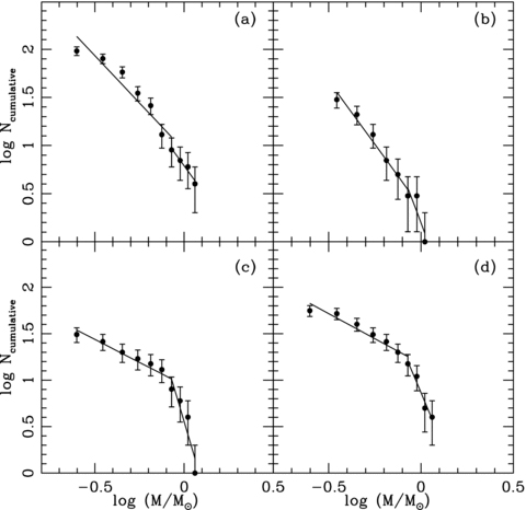
CMFs of YSOs in the (a) cluster, (b) BRC NW, (c) BRC 13 and (d) BRC 14 regions. Error bars represent ± errors.
CMFs of the YSOs in the cluster and BRC regions.
| Region | CMF in the mass range | |
| (0.8 ≤M/M⊙≤ 1.2) | (0.2 ≤M/M⊙≤ 0.8) | |
| Cluster | −2.54 ± 0.40 | −1.97 ± 0.28 |
| BRC NW | −5.06 ± 3.18 | −2.63 ± 0.21 |
| BRC 13 | −6.45 ± 2.01 | −0.98 ± 0.14 |
| BRC 14 | −4.69 ± 0.75 | −1.08 ± 0.14 |
| Region | CMF in the mass range | |
| (0.8 ≤M/M⊙≤ 1.2) | (0.2 ≤M/M⊙≤ 0.8) | |
| Cluster | −2.54 ± 0.40 | −1.97 ± 0.28 |
| BRC NW | −5.06 ± 3.18 | −2.63 ± 0.21 |
| BRC 13 | −6.45 ± 2.01 | −0.98 ± 0.14 |
| BRC 14 | −4.69 ± 0.75 | −1.08 ± 0.14 |
8 STAR FORMATION SCENARIO IN W5 E H ii
The W5 E H ii region is an excellent example of triggered star formation. The presence of the central O7 MS star HD 18326 and several bright-rim like structures makes this region an interesting object to study triggered star formation. This region contains two of the BRCs catalogued in SFO 91. The millimetre line study by Niwa et al. (2009) has revealed the presence of a 13CO cloud and C18O cores on the eastern and northern sides of the region, but there is no evidence for clouds on the southern side. They also found high-density clumps in the BRC NW region. Karr & Martin (2003) concluded that the exciting O stars and YSOs along the edges of the whole W5 E H ii region belong to two different generations. Based on the expansion velocity of the H ii region and the evolutionary stages of the IRAS YSOs, they concluded that the time-scale is consistent with the triggering by the RDI process.
In our earlier work (Paper I and Paper II), we have studied the star formation scenario in and around BRCs using the YSOs selected on the basis of Hα emission and NIR excess, and found evidence for triggered star formation around BRCs 13 and 14. Nakano et al. (2008) detected several Hα-emission stars in the W5 E H ii region. They found that the young stars near the exciting stars are systematically older (∼4 Myr) than those near the edge of the H ii region (∼1 Myr) and concluded that the formation of stars proceeded sequentially from the centre of the H ii region to the eastern bright rims. Based on the observations of IR-excess stars, we proposed in Paper II the occurrence of a series of RDI events in this particular region.
Koenig et al. (2008) have carried out an extensive Spitzer survey of the whole IC 1848 region. On the basis of the large-scale distribution of YSOs selected using Spitzer data, they found that the ratio of Class II to Class I sources within the H ii region cavity is approximately seven times higher compared to the regions associated with the molecular cloud. They attributed this difference to an age difference between the two locations and concluded that there exist at least two distinct generations of stars in the region. They stated that the triggering is a plausible mechanism to explain the multiple events of star formation and suggested that the W5 E H ii region merits further investigation.
Earlier works studying the star formation scenario in the region were often qualitative (e.g. Karr & Martin 2003; Koenig et al. 2008). Some were quantitative studies, but they were based on a smaller sample of stars (e.g. Paper I; Nakano et al. 2008; Paper II). Since in this work we have a larger data base, it will be worthwhile studying the global scenario of the star formation in the region. In the following sections, we shall study the star formation scenario in the cluster as well as around the BRCs.
8.1 Cluster region
The CMD of the identified YSOs (Fig. 9a) and the statistically cleaned CMD (Fig. 11) reveal a non-coeval star formation in the cluster region. The age distribution is shown in Fig. 14. The mean age of the YSOs is estimated to be 1.26 ± 0.69 Myr. This is smaller than the average age of the YSOs obtained by Nakano et al. (2008, age ∼4 Myr). Nakano et al. (2008) have used only Hα-emission stars, while the present sample is larger, including NIR- and MIR-excess stars in addition. To estimate the age of the Hα-emission stars, Nakano et al. (2008) used PMS isochrones by Palla & Stahler (1999), whereas we have used those by Siess et al. (2000). The use of different PMS evolutionary models can introduce a systematic shift in the age estimation.
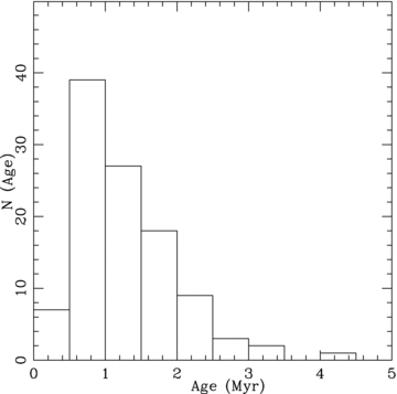
Histogram of the age distribution for the YSOs in the cluster region.
8.2 BRC regions
BRCs are considered to be a sort of remnant clouds originating from the dense parts (cores) in an inhomogeneous molecular cloud. So, if the original core were big enough, the resultant BRC would have undergone a series of RDI events (Kessel-Deynet & Burkert 2003), leaving an elongated distribution of young stars. The distribution and evolutionary stages of such YSOs could be used to probe the star formation history in the H ii regions. Using Spitzer observations, Koenig et al. (2008) have identified clustered and distributed populations of YSOs in the W5 E H ii region (see their fig. 12). The clustered population shows a nice alignment of Class II sources towards the directions of BRCs from the ionization sources. In Paper II, we also examined the global distribution of YSOs, the radial distribution of AV as well as the amount of NIR excess Δ(H−K), defined as the horizontal displacement from the middle reddening vector in the NIR-CC diagram (see Fig. 6), in BRCs 13 and 14 regions. On the basis of these distributions, star formation was found to have propagated from the ionizing source in the direction of the BRCs.
Fig. 15 shows the global distribution of clustered YSOs selected from the study of Koenig et al. (2008), in the whole W5 E H ii region, which indicates an alignment of YSOs towards the direction of the BRCs. Fig. 16 shows the radial variation of Δ(H−K) and AV of the YSOs located within the strip towards the direction of the BRC NW region. The distribution reveals higher AV values near the BRC NW region.
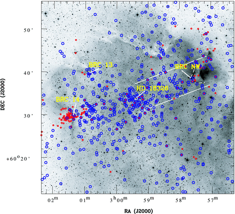
Global distribution of YSOs in the W5 E H ii region. The small red circles show the locations of NIR-excess sources, whereas the large blue circles (see the online version) show the YSOs identified using the Spitzer observations (see text).
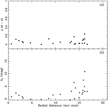
Variation in NIR excess Δ(H − K) (upper panel) and AV (lower panel) for the IR-excess stars in the strip towards BRC NW as a function of the distance from the ionizing source (HD 18326) of the W5 E H ii region.
On the basis of the global distribution of YSOs in the region and the radial distribution of the amount of the NIR excess Δ(H−K) and AV in the region (cf. Figs 16 and 17 and figs 6–8 of Paper II) as well as the age distribution of YSOs, it seems that a series of RDI processes proceeded in the past from near the central O star towards the present locations of the BRCs.
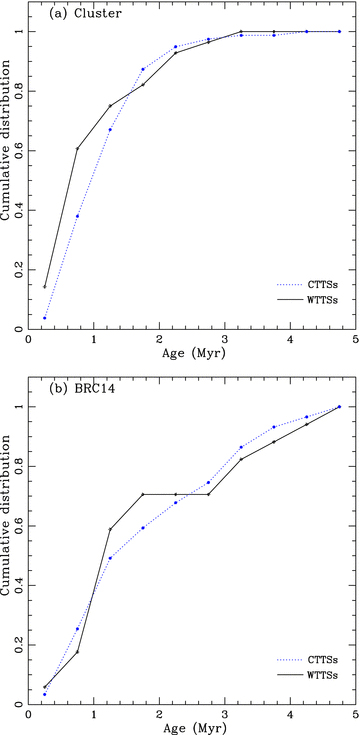
Cumulative age distribution of Class II (CTTSs) and Class III (WTTSs) sources in the (a) cluster and (b) BRC 14 region.
8.2.1 Small-scale sequential star formation (S4F)
There has been qualitative evidence for the S4F hypothesis such as an asymmetric distribution of probable TTSs (Ogura et al. 2002) and of the properties of NIR-excess stars (Matsuyanagi et al. 2006). Paper I and Paper II presented some quantitative evidence on the basis of BVIC photometry. In this study, the sample of YSOs is significantly larger as compared to that used in Paper I and Paper II. To further verify the S4F hypothesis, we follow the approach as given in Paper I and Paper II. We have divided the YSOs associated with BRCs into two groups: those lying inside/on the rim (i.e. stars embedded or projected on to the molecular cloud/lying on the rim) and outside the rim (i.e. stars lying outside the rim in the projected H ii region) (see e.g. fig. A1 of Paper II for BRCs 13 and 14). The mean age has been calculated for these regions. Since the ionizing source of the BRCs studied here has a maximum MS lifetime of 4–5 Myr, therefore the sources having age greater than 5 Myr cannot be expected as the products of the triggered star formation. They might have formed spontaneously in the original molecular cloud prior to the formation of the H ii region. Some of them may be background stars; larger distances make them look older in the CMD. Therefore, while calculating the mean age we have not included those stars. The results are given in Table 5, which shows that in all the BRCs, the YSOs lying on/inside the rim are younger than those located outside it. The above results are exactly the same as those obtained in Paper I and Paper II. Therefore, the present results further confirm the S4F hypothesis. As in Paper I and Paper II, we again find a large scatter in the stellar age in spite of a clear trend of the mean age. Possible reasons for the scatter, as discussed in earlier papers, include photometric errors, errors in extinction correction, light variation of young stars, drift of stars due to their proper motions, binarity of the stars, etc. Photometric errors and light variation as big as 0.5 mag would affect stellar ages by 0.25 dex, so they do not seem to be the major reason for the scatter. As for the extinction correction, it probably does not affect the results much, since in the V, (V−IC) CMD the reddening vector is nearly parallel to the isochrones. As discussed in Paper I and Paper II, we speculate that the proper motions of the newly born stars may probably be the main cause of the scatter.
Mean age inside/on the rim and outside the rim.
| Region | Mean age (Myr) | |
| Inside/on the rim (number of sources) | Outside the rim (number of sources) | |
| BRC NW | 0.92 ± 0.56 (12) | 1.29 ± 0.54 (19) |
| BRC 13 | 1.61 ± 1.41 (10) | 2.44 ± 1.37 (24) |
| BRC 14 | 1.01 ± 0.73 (18) | 2.32 ± 1.22 (58) |
| Region | Mean age (Myr) | |
| Inside/on the rim (number of sources) | Outside the rim (number of sources) | |
| BRC NW | 0.92 ± 0.56 (12) | 1.29 ± 0.54 (19) |
| BRC 13 | 1.61 ± 1.41 (10) | 2.44 ± 1.37 (24) |
| BRC 14 | 1.01 ± 0.73 (18) | 2.32 ± 1.22 (58) |
9 EVOLUTION OF DISCS OF T TAURI STARS
Hα emission and IR excess are important signatures of young PMS stars. These signatures in CTTSs indicate the existence of a well-developed circumstellar disc actively interacting with the central star. Strong Hα emission [equivalent width (EW) > 10 Å] in CTTSs is attributed to the magnetospheric accretion of the innermost disc matter on to the central star (Edwards et al. 1994; Hartmann, Hewett & Calvet 1994; Muzerolle, Calvet & Hartmann 2001 and references therein). On the other hand, the weak Hα emission (EW < 10 Å) in weak-line TTSs (WTTSs), which lack discs (or, at least inner discs), is believed to originate from their chromospheric activity (e.g. Walter et al. 1988; Martín 1998). In the 1990s, a large number of WTTSs were found in and over wide areas around T associations by X-ray surveys with the ROSAT, which led to active studies on the nature of the so-called dispersed WTTSs.
The ‘standard model’ (Kenyon & Hartmann 1995) postulates that the CTTSs evolve to the WTTSs by losing their circumstellar disc (or, at least its inner part). The age distribution derived from the Hertzsprung–Russell (HR) diagram of the Taurus region indicates that the WTTSs are systematically older than the CTTSs, but the statistical significance is low (Kenyon & Hartmann 1995; Hartmann 2001; Armitage et al. 2003). Bertout et al. (2007) concluded that the observed age and mass distribution of CTTSs and WTTSs in the Taurus–Auriga T association can be explained by assuming that a CTTS evolves into a WTTS. In Paper II, we compared the age distribution of CTTSs with that of WTTSs associated with several BRCs and supported the conclusion of Bertout et al. (2007).
On the other hand, there have also been many observations which claimed that the CTTSs and WTTSs are coeval and have an indistinguishable age distribution (e.g. Walter et al. 1988; Lawson, Fiegelson & Huenemoerder 1996; Gras-Velá zquez & Ray 2005). From the analyses of the HR diagram of the CTTSs and WTTSs in Chamaeleon I, Lawson et al. (1996) concluded that some stars may be born even almost discless or lose the disc at very early stages (age <1 Myr).
In this work, we have derived the age of 79, 26, 29 and 59 Class II and 27, 5, 5 and 17 Class III sources in the cluster, BRC NW, BRC 13 and BRC 14 regions, respectively. Assuming that all the identified Class II and Class III stars are CTTSs and WTTSs, respectively, we can study the possible evolution of the TTSs. The advantage of our sample in addressing this issue is that the stars are spatially, that is, three-dimensionally, very close to each other, so there should be no problem of the distance difference, contrary to extended T associations. Here we would like to caution the readers that although we have attempted to clean the Class III sample from sources not belonging to W5, however, to confirm the WTTS nature of these sources in the absence of spectral information, such as the measurement of the lithium absorption line, is difficult.
Since data for Class III sources in the BRC NW and BRC 13 regions are not statistically significant, in Fig. 17 we show the cumulative distribution of Class II and Class III sources in the cluster and BRC 14 region only. Fig. 17 indicates that both the Class III and Class II sources have rather similar distributions. A Kolmogorov–Smirnov test for the combined sample of the cluster and BRC 14 region confirms the statement that the cumulative distributions of Class II sources (CTTSs) and Class III sources (WTTSs) are different only at a confidence level of 50 per cent. Hence, we can conclude that both the samples have rather similar distributions with practically indistinguishable age distributions. This result is in contradiction to that of Bertout et al. (2007) for the Taurus–Auriga T association and that of Paper II that WTTSs are older than CTTSs and CTTSs evolve into WTTSs, and it is in agreement with those which claim that the CTTSs and WTTSs are coeval and have indistinguishable properties. Here we have to keep in mind that the classification of CTTSs and WTTSs in this work is based on the Spitzer MIR observations, whereas in Paper II and in Bertout et al. (2007), the classification was based on the EWs of Hα-emission stars. Hα surveys may fail to detect Class III sources which have smaller EWs, whereas those sources can be identified using the MIR observations. Here it is worthwhile to point out that the Class III sources by Koenig et al. (2008) were identified on the basis of all four Spitzer IRAC bands (3.6, 4.5, 5.8 and 8.0 μm). The detection of Class III sources would be suppressed because of less sensitivity at 5.8- and 8.0-μm bands and also because of the very bright, variable background at these wavelengths in W5. Koenig et al. (2008) have stated that their photospheric sample is only 90 per cent complete to 2 M⊙ in general in W5 and to 8 M⊙ on regions of bright background emission (e.g. the BRCs studied in this paper). This fact is evident in the V/(V−I) CMD (Fig. 7) by comparing the number of Class II sources with the number of Class III sources fainter than the 20th magnitude in the V band.
10 CONCLUSIONS
In this paper, we have made VIC photometric studies of the newly the identified central cluster of W5 E H ii. NIR data from 2MASS and MIR data from the IRAC/MIPS of the Spitzer telescope have also been added to consider the properties of the cluster. Also, by incorporating Spitzer data, we have re-analysed the properties (age, spatial distribution, etc.) of the YSOs in W5 E H ii with special emphasis on the three BRC regions. We obtained the following as the main conclusion of this work.
The central cluster has a distance of ∼2.1 kpc, a radius of 6 arcmin and a mean age of ∼1.3 Myr. The reddening law is normal. The star formation in the cluster region is found to be non-coeval, with an age spread of ∼5 Myr. The slope of the IMF within the cluster region in the mass range 0.4 ≤M/M⊙≤ 30 is found to be Γ=−1.29 ± 0.04, which is comparable to the Salpeter value. In the mass range of 0.2 ≤M/M⊙≤ 0.8, the CMFs of the YSOs associated with the three BRCs show a break in the slope at ∼0.8 M⊙. The CMFs indicate that the cluster region and BRC NW have relatively more low-mass YSOs in the mass range 0.2 ≤M/M⊙≤ 0.8.
The distribution of the YSOs in the W5 E H ii region indicates that they are globally aligned with the ionizing source towards the BRCs. A comparison of the average age of the YSOs lying on/inside and outside the bright rim indicates a quantitative age gradient in the sense that the YSOs located on/inside the rim are younger than those located outside the rim. The results are similar to those reported in Paper I and Paper II. These results confirm the S4F hypothesis. The globally aligned distribution of the YSOs indicates that a series of RDI events took place in the past from near the central ionizing source to the periphery of the H ii region.
In this study, it is found that the age distributions of the Class II and Class III sources are the same. This result is in accordance with the results which claimed that the CTTSs and the WTTSs are coeval and have indistinguishable age distributions (e.g. Walter et al. 1988; Lawson et al. 1996; Gras-Velá zquez & Ray 2005).
The authors are grateful to the anonymous referee for useful comments that improved the content of this paper. We are thankful to the Kiso Observatory, IAO and ARIES for allotting the observing time. We also thank the staff of the Kiso Observatory (Japan), IAO, Hanle, and its remote control station CREST, Hosakote, for their assistance during observations. This publication makes use of data from the 2MASS, which is a joint project of the University of Massachusetts and the Infrared Processing and Analysis Center/California Institute of Technology, funded by the National Aeronautics and Space Administration and the National Science Foundation. NC is thankful for the financial support for this study through the fellowships granted by the DST and CSIR, India.
REFERENCES
SUPPORTING INFORMATION
Additional Supporting Information may be found in the online version of this article:
Table 3. The B, V and IC photometric data along with their position, mass and age for the YSOs in the cluster and BRC regions.
Please note: Wiley-Blackwell Publishing are not responsible for the content or functionality of any supplementary materials supplied by the authors. Any queries (other than missing material) should be directed to the corresponding author for the article.
