


Abstract
We study the BL Lac objects detected in the 1-year all-sky survey of the Fermi satellite, with an energy spectral slope αγ in the 0.1–100 GeV band greater than 1.2. In the αγ versus γ-ray luminosity plane, these BL Lacs occupy the region populated by flat spectrum radio quasars (FSRQs). Studying the properties of their spectral energy distributions (SEDs) and of their emitting lines, we find that several of these BL Lacs have an SED similar to FSRQs and that they do have broad lines of large equivalent width (EW), and should be reclassified as FSRQs even adopting the current phenomenological definition (i.e. EW of the emitting line greater than 5 Å). In other cases, even if the EW is small, the emitting lines can be as luminous as in quasars, and again their SED is similar to the SED of FSRQs. Sources classified as BL Lacs with an SED appearing as intermediate between BL Lacs and FSRQs also have relatively weak broad emission lines and small EW, and can be considered as transition sources. These properties are confirmed also by model fitting that allows us to derive the relevant intrinsic jet parameters and the jet power. This study leads us to propose a physical distinction between the two classes of blazars, based on the luminosity of the broad-line region measured in Eddington units. The dividing line is of the order of LBLR/LEdd∼ 5 × 10⁻⁴, in good agreement with the idea that the presence of strong emitting lines is related to a transition in the accretion regime, becoming radiatively inefficient below a disc luminosity of the order of 1 per cent of the Eddington one.
1 INTRODUCTION
Among the blazars detected by the Large Area Telescope (LAT) onboard the Fermi satellite after 11 months of all-sky survey (Abdo et al. 2010a, hereafter A10) there are roughly an equal number of sources identified as BL Lac objects and flat spectrum radio quasars (FSRQs). The corresponding catalogue of active galactic nuclei (AGN) detected at high Galactic latitude (|b| > 10°) is called the First LAT AGN Catalogue (1LAC). In general, the LAT-detected BL Lac objects and FSRQs separate quite well in the γ-ray spectral index –γ-ray luminosity plane (αγ−Lγ, where αγ is the energy spectral index), in agreement with the early results of the 3-month all-sky survey of Fermi/LAT, which contained only 1/7 of the blazars in the 1LAC catalogue (Ghisellini, Maraschi & Tavecchio 2009, hereafter GMT09). On the other hand, there are a number of sources, classified as BL Lac objects, located in the region of the plane preferentially ‘inhabited’ by FSRQs: these are BL Lacs with a relatively steep spectrum (i.e. αγ > 1.2). These ‘intruders’ have been classified as BL Lac objects on the basis of the ‘historical’ distinction among BL Lacs and FSRQs, i.e. by means of the equivalent width (EW) of their emission lines (see e.g. Urry & Padovani 1995). Objects with a rest-frame EW < 5 Å are called BL Lacs. This definition has the obvious advantage of being simple and of immediate use for an observational characterization of the object. On the other hand, the optical continuum of most blazars is relativistically enhanced by beaming, and very variable. In several cases a small EW does not imply emission lines of low luminosity, being simply the result of a particularly beamed non-thermal continuum. On the opposite side, an EW greater than 5 Å may be the result of a particularly low state of the beamed continuum in a source of intrinsically weak lines. A division based on the EW of emission lines does measure the relative importance of the beamed non-thermal continuum and the underlying thermal emission, but after the discovery that most of the non-thermal emission is at γ-ray energies, we know that the optical non-thermal flux very often is a minor contribution to the total, bolometric, non-thermal output. Therefore, the EW alone is not a good indicator of the relative importance of the two contributions.
Up to now, we have constructed samples of BL Lacs as well as of FSRQs in order to study their properties and their possible differences, and adopt the classical, EW-based, sub-division. If the aim is to study intrinsically physical properties, this may be dangerous, since with the EW classification we may – for instance – classify as a BL Lac object a source with very luminous lines, typical of an FSRQ, only because at the time of the spectroscopic observations leading to the measurement of the EW the optical non-thermal flux was particularly intense. For illustration, let us take the case of PKS 0208−512. It has an observed Mg ii emission line of EW ∼ 5 Å (2.5 in the rest frame), whose luminosity is close to 1044 erg s−1, stronger than in some FSRQs. This object is classified as a BL Lac, but all its physical properties are resembling FSRQs.
We therefore believe that a new classification scheme is needed, based on a physical property of the source. We suggest a division based on the luminosity of the broad emission lines, normalized to the corresponding Eddington luminosity, the natural luminosity scale. Normalizing in this way allows us to compare objects of different black hole masses. This division implies estimation of the black hole mass, which is not a directly observable quantity. On the other hand, in recent years, the establishing of correlations between (i) the luminosity of the bulge of the host galaxy and the black hole mass (Magorrian et al. 1998; Bentz et al. 2009), (ii) the correlation between the dispersion velocity and the black hole mass (Ferrarese & Merritt 2000; Gültekin et al. 2009), and (iii) the correlation between the luminosity of the continuum at selected frequencies and the size of the broad-line region (BLR; Vestergaard 2002; Decarli et al. 2010 and references therein) made the estimate of the black hole mass much easier. Furthermore, in specific cases, very powerful blazars do have their IR–optical–UV continuum dominated by a thermal component produced by their accretion disc: modelling it with a standard Shakura & Sunyaev (1973) disc allows us to find both the black hole mass and the accretion rate.
We then investigate if the ‘intruder’ BL Lacs in the αγ−Lγ plane have intrinsically weak emission lines (in Eddington units) or if instead their EW is only a consequence of a particularly enhanced non-thermal continuum, or else if they are transition objects, with intermediate values of the broad-line luminosity.
We use a cosmology with h=ΩΛ = 0.7 and ΩM = 0.3, and use the notation Q = 10XQx in cgs units (except for the black hole masses, measured in solar mass units).
2 The FERMI BLAZARS’ DIVIDE ONE YEAR AFTER
Fig. 1 shows the energy spectral index αγ as a function of the (K-corrected; see GMT09) γ-ray luminosity Lγ for the FSRQs and BL Lacs on the 1LAC sample of known redshift. This figure can be compared with the same one in GMT09 reporting the bright blazars of the LAT Bright AGN Sample (LBAS, Abdo et al. 2009, hereafter A09) for the 3-month all-sky survey. In that figure there was a specific γ-ray luminosity dividing FSRQs and BL Lacs, around a few times 1046 erg s−1, interpreted as a consequence of the changing accretion regime of the underlying accretion disc from radiatively efficient to inefficient, or, in other words, from a standard Shakura & Sunyaev (1973) disc to an advection dominated accretion flow (ADAF) one. As remarked in GMT09, the appearance of the dividing luminosity required that all the bright blazars in the LBAS sample have black holes of the same mass and similar beaming factors. This is approximately appropriate when considering the brightest sources, but when the decreased limiting flux allows us to explore smaller luminosities both for FSRQs and for BL Lacs, then it is likely that the corresponding black hole mass (and/or the beaming factor) is smaller, and the dividing luminosity gets spread into a larger range of values (as large as the spread in black hole masses and beaming factors). This explains why, in Fig. 1, no dividing luminosity is present. A comparison with fig. 1 of GMT09 shows that all the most luminous blazars were present also in LBAS: the decreased flux limit did not lead to the discovery of any new more powerful object. Furthermore, differently from fig. 1 of GMT09, there is now no trend between the minimum luminosities and spectral index, although, at low luminosities, flat γ-ray spectra BL Lacs are more numerous than sources with a relatively steep αγ. This is likely due to LAT being more sensitive to flat spectra than to steep ones (see fig. 9 of A10). As already noted in GMT09, a correlation between αγ and Lγ is not expected, since at low γ-ray luminosities we expected the detection of FSRQs of lower black hole masses and smaller beaming. This fills the top-left part of the αγ−Lγ plane.
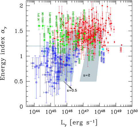
The energy spectral index αγ as a function of the γ-ray luminosity Lγ in the band 0.1–10 GeV for all blazars with known redshift present in the 1LAC sample. The filled circles (red in the electronic version) are FSRQs; empty (blue) squares are BL Lacs with αγ < 1.2 and filled (green) squares are sources classified as BL Lacs in the 1LAC sample with αγ > 1.2. In addition, the two larger (cyan) circles are 0235+164 and 0426−380, classified as BL Lacs, that have Lγ > 1048 erg s−1. The horizontal grey line marks αγ = 1.2. The two grey regions illustrate how the corresponding grey area shown in Fig. 2 would lie assuming a redshift of 0.5 or 2, as indicated.
The majority of BL Lac sources are characterized by a relatively flat αγ (αγ≲ 1.2), but there are several exceptions. Some of these BL Lacs, however, have been classified as such because the EW of their broad lines (that are indeed present) is less than 5 Å. We discussed in GMT09 the cases of PKS 0537−441, AO 0235+164 and PKS 0426−380, that do have broad lines visible in their low emission states (see Sbarufatti et al. 2005 for PKS 0426−380; Pian et al. 2002 for PKS 0537−441; Raiteri et al. 2007a for AO 0235+164). Another example is 0208−512: it was observed to have an Mg ii broad line with EW ∼ 5 Å (2.5 Å in the rest frame), but with a very large luminosity (∼1044 erg s−1; Scarpa & Falomo 1997). Therefore 0208−512 (and the other mentioned sources) are FSRQs whose non-thermal continuum is enhanced so much to make the very luminous broad lines almost disappear, and not BL Lac objects with genuinely weak lines. Not appreciating this point may cause some confusion when comparing FSRQs and BL Lacs.
With respect to the LBAS sample, the number of sources classified as BL Lacs but of unknown redshift increased: from the source list in A10 there are 159 sources classified as ‘BLL’ with no redshift (in the ‘clean’ sample), excluding the sources classified as of ‘unknown’ type.
In Fig. 2, we show the energy spectral index αγ versus the 0.1–100 GeV photon flux of these 159 ‘BLL’ sources. Of these 159 sources, 54 have αγ≥ 1.2 (80 if we include the sources with ‘uncertain’ classification). Fig. 2 shows in grey the area where most of the sources are. Exceptions at large photon fluxes are labelled, and we here briefly comment on these sources.

Energy index αγ versus γ-ray flux in the 0.1–100 GeV energy band for the sources classified in the clean 1LAC catalogue as ‘BLL’ (and excluding the ones classified as ‘unknown’). The plotted 0.1–100 GeV photon flux has been calculated from the 1–100 GeV flux listed in A10, using the corresponding spectral index. The grey region corresponds to the two grey areas in Fig. 1. The (green) squares are the 56 sources with αγ≥ 1.2 (this limit is shown by the horizontal line). See text for a brief comment about the labelled sources that are located outside the grey region.
PKS 1424+240 and PG 1553+113 have been detected at TeV energies [see Ong et al. (2009) and Teshima et al. (2009) for 1424+240, and Aharonian et al. (2006) and Albert et al. (2007) for PG 1553+113; see also Prandini et al. (2010)], and very likely also 3C 66A (Acciari et al. 2009), although there can be a contamination from the nearby 3C 66B radio-galaxy (see the discussion in Tavecchio & Ghisellini 2009). The redshift of 3C 66A is uncertain, even if a value of z = 0.444 is commonly used. Due to the TeV detection, these three sources cannot lie at very large redshift although z up to ∼0.7 would be possible (see Tavecchio et al. 2010 for PKS 1424+240 modelled assuming z = 0.67).
For B3 0814+425, the NED data base gives z = 0.53, quoting Sowards-Emmerd et al. (2005) from Sloan Digital Sky Survey (SDSS) data. However, the inspection of the SDSS spectrum does not confirm this redshift (nor the other quoted value, z = 1.07).
Finally, there is no information for the redshift of CRATES J1542+6129 = GB6 J1542+6129. It has been imaged by the SDSS, but no spectrum is available.
If we assign to all sources in the grey area of Fig. 2 a given redshift, we can see the corresponding region in Fig. 1. We show this for two redshifts: z = 0.5 and z = 2, as labelled. It can be seen that in the case of z∼ 0.5 the BLL sources of unknown redshift would lie in the region already occupied by the other BL Lacs, while they would be ‘outliers’ if the redshift is as large as 2 (see also the discussion in A10).
In other words, if the BLL sources in the 1LAC catalogue with unknown redshift turn out to be at z≲ 0.5–1, then they will fit in the phenomenological blazar sequence [i.e. they would be BL Lacs of low and moderate luminosity, with the majority having a flat γ-ray slope (i.e. αγ < 1–1.2); Fossati et al. 1998; Donato et al. 2001], while they would pose a problem if their redshift is larger. We will further discuss this point in Section 5.
2.1 The ‘intruder’ BL Lac sample
We consider all the sources classified as BL Lacs in the ‘clean’ 1LAC sample (defined as BL Lacs with |b| > 10°, detected with a TS significance larger than 25 (TS stands for Test Statistics; see Mattox et al. 1996 for the definition; TS = 25 approximately corresponds to 5σ), whose identification is secure and unique. We selected the sources of known redshift with a γ-ray energy spectral index αγ larger than 1.2, corresponding to a photon spectral index Γγ > 2.2. The resulting 28 BL Lac objects are listed in Table 1. At the end of the same table we add the two BL Lacs (0235+164 and 0426−380) that were ‘intruders’ because of their extremely large γ-ray luminosity (i.e. Lγ > 1048 erg s−1), even if their spectral index was somewhat flatter than αγ = 1.2. All these objects are shown and labelled in Fig. 1, and correspond to the filled squares.
Fγ in the LAT band (0.1–100 GeV) in units of 10−8 ph cm−2 s−1. Lγ, in the same band, is K-corrected and in units of erg s−1. *: no Swift observations. Sources whose name is in italics are present in Ghisellini et al. (2010a, hereafter G10), and some of them are present in Tavecchio et al. (2010).
| Fermi name | Coordinates (J2000.0) | Alias | z | Γγ | Fγ | log Lγ |
| 1FGL J0058.0+3314 | 00 58 32.07 +33 11 17.2 | GB6 0058+3311 | 1.371 | 2.33 ± 0.11 | 3.13 | 47.36 |
| 1FGL J0112.0+2247 | 01 12 05.82 +22 44 38.8 | TXS 0109+224 | 0.265 | 2.23 ± 0.05 | 7.81 | 45.99 |
| 1FGL J0210.6−5101 | 02 11 13.18 +10 51 34.8 | PKS 0208−512 | 1.003 | 2.37 ± 0.04 | 14.59 | 47.69 |
| 1FGL J0522.8−3632 | 05 22 57.98 −36 27 30.9 | PKS 0521−36 | 0.055 | 2.60 ± 0.06 | 11.54 | 44.45 |
| 1FGL J0538.8−4404 | 05 38 50.35 −44 05 08.7 | PKS 0537−441 | 0.892 | 2.27 ± 0.02 | 37.77 | 48.00 |
| 1FGL J0557.6−3831 | 05 58 06.47 −38 38 31.7 | PMN 0558−3839 | 0.302 | 2.32 ± 0.17 | 1.74 | 45.44 |
| 1FGL J0757.2+0956 | 07 57 06.64 +09 56 34.9 | PKS 0754+100 | 0.266 | 2.39 ± 0.08 | 4.86 | 45.73 |
| 1FGL J0811.2+0148 | 08 11 26.71 +01 46 52.2 | PKS 0808+019 | 1.148 | 2.45 ± 0.12 | 2.97 | 47.08 |
| 1FGL J0831.6+0429 | 08 31 48.88 +04 29 39.1 | PKS 0829+046 | 0.174 | 2.50 ± 0.07 | 7.35 | 45.39 |
| 1FGL J0854.8+2006 | 08 54 48.87 +20 06 30.6 | OJ 287 | 0.306 | 2.38 ± 0.07 | 7.03 | 45.18 |
| 1FGL J0910.7+3332 | 09 10 37.04 +33 29 24.4 | TON 1015 | 0.354 | 2.32 ± 0.14 | 2.00 | 45.66 |
| 1FGL J1000.1+6539 | 09 58 47.25 +65 33 54.8 | TXS 0954+658 | 0.367 | 2.51 ± 0.16 | 2.59 | 45.69 |
| 1FGL J1012.2+0634 | 10 12 13.35 +06 30 57.2 | PMN 1012+0630 | 0.727 | 2.30 ± 0.2 | 1.51 | 46.55 |
| 1FGL J1027.1−1747 | 10 26 58.52 −17 48 58.5 | BZB 1026−1748* | 0.114 | 2.32 ± 0.29 | 1.22 | 44.62 |
| 1FGL J1058.1−8006 | 10 58 43.40 −80 03 54.2 | PKS 1057−79 | 0.581 | 2.45 ± 0.1 | 6.26 | 46.66 |
| 1FGL J1150.2+2419 | 11 50 19.21 +24 17 53.9 | B2 1147+24* | 0.2? | 2.25 ± 0.12 | 2.08 | 45.17 |
| 1FGL J1204.3−0714 | 12 04 16.66 −07 10 09.0 | WGA 1204.2−0710* | 0.185 | 2.59 ± 0.23 | 2.07 | 44.99 |
| 1FGL J1341.3+3951 | 13 41 05.10 +39 59 45.4 | B2 1338+40 | 0.172 | 2.45 ± 0.21 | 1.29 | 44.94 |
| 1FGL J1522.6−2732 | 15 22 37.68 −27 30 10.8 | PKS 1519−273 | 1.294 | 2.25 ± 0.08 | 4.94 | 47.55 |
| 1FGL J1558.9+5627 | 15 58 48.29 +56 25 14.1 | TXS 1557+565* | 0.3 | 2.24 ± 0.13 | 2.91 | 45.73 |
| 1FGL J1751.5+0937 | 17 51 32.82 +09 39 00.7 | PKS 1749+096 | 0.322 | 2.29 ± 0.05 | 12.22 | 46.43 |
| 1FGL J1800.4+7827 | 18 00 45.68 +78 28 04.0 | S5 1803+78 | 0.68 | 2.35 ± 0.07 | 6.24 | 46.94 |
| 1FGL J1807.0+6945 | 18 06 50.68 +69 49 28.1 | 3C 371 | 0.05 | 2.60 ± 0.08 | 7.70 | 44.29 |
| 1FGL J2006.0+7751 | 20 05 31.00 +77 52 43.2 | S5 2007+77 | 0.342 | 2.42 ± 0.16 | 3.00 | 45.81 |
| 1FGL J2202.8+4216 | 22 02 43.29 +42 16 40.0 | BL LAC | 0.069 | 2.38 ± 0.04 | 16.81 | 44.97 |
| 1FGL J2217.1+2423 | 22 17 00.83 +24 21 46.0 | B2 2214+24 | 0.505 | 2.63 ± 0.12 | 4.97 | 46.36 |
| 1FGL J2243.1−2541 | 22 43 26.36 −25 44 27.0 | PKS 2240−260 | 0.774 | 2.32 ± 0.09 | 3.44 | 46.75 |
| 1FGL J2341.6+8015 | 23 40 54.28 +80 15 16.1 | FRBA J2340+8015 | 0.274 | 2.21 ± 0.08 | 4.21 | 45.83 |
| 1FGL J0238.6+1637 | 02 38 38.93 +16 36 59.3 | PKS 0235+164 | 0.94 | 2.14 ± 0.02 | 43.4 | 48.24 |
| 1FGL J0428.6−3756 | 04 28 40.42 −37 56 19.6 | PKS 0426−380 | 1.111 | 2.13 ± 0.02 | 31.5 | 48.18 |
We will characterize the SED of all the 30 BL Lacs of Table 1 and search for existing data on the luminosity of their broad lines, if present.
3 SWIFT OBSERVATIONS AND ANALYSIS
Several blazars studied in this paper were observed by the Swift satellite. These objects are listed in Table 2 (X-ray data) and Table 3 (optical/UV data). Even when they were performed during the 11 months of the 1LAC survey, they correspond to a ‘snapshot’ of the optical–X-ray state of the source, while the γ-ray data are an average over the 11 months. Given the very rapid blazar variability, the SEDs constructed in this way should be considered, in all cases, not simultaneous (even when the Swift Ultraviolet Optical Telescope (UVOT) and X-Ray Telescope (XRT) data are indeed simultaneous).
Summary of XRT observations. The observation date column indicates the date of a single snapshot or the years during which multiple snapshots were performed. The corresponding note reports the complete set of observations integrated. The column ‘Exp’ indicates the effective exposure in ks, while NH is the Galactic absorption column in units of 1020 cm−2 from Kalberla et al. (2005). Γ is the photon index of the power-law model [F(E) ∝E−Γ],  is the observed (absorbed) flux. The two last columns indicate the results of the statistical analysis: the last column contains the degrees of freedom, while the last but one column displays the reduced
  or the value of the likelihood (Cash 1979).
| Name | Obs. date (yyyy-mm-dd) | Exp (ks) | NH (1020 cm−2) | Γ |  (10−13 erg cm−2 s−1) (10−13 erg cm−2 s−1) |  /Cash /Cash | d.o.f. |
| 0058+3311 | 2009-08-21 | 8.7 | 4.89 | 1.1 ± 0.4 | 3.3 ± 0.5 | −/47 | 36 |
| 0521−36 | 2005–2010a | 32.4 | 3.32 | 1.61 ± 0.02 | 203 ± 2 | 1.2/– | 280 |
| 0754+100 | 2007–2010b | 20.3 | 2.21 | 1.63 ± 0.05 | 54 ± 1 | 0.95/– | 65 |
| 0808+019 | 2007–2009c | 19.6 | 3.84 | 2.2 ± 0.3 | 4.2 ± 0.3 | 0.2/– | 3 |
| 0829+046 | 2006–2010d | 27.9 | 2.41 | 1.56 ± 0.08 | 19.4 ± 0.6 | 0.65/– | 30 |
| 0954+658 | 2006–2010e | 57.6 | 5.47 | 1.89 ± 0.07f | 33.6 ± 0.5 | 1.0/– | 112 |
| 1012+0630 | 2010g | 4.8 | 1.97 | 2.0 ± 0.3 | 4.6 ± 0.6 | –/47 | 45 |
| 1026−1748 | 2010-07-24 | 0.01 | 6.42 | 2(fixed) | <30h | –/– | – |
| 1204−0710 | 2010-08-09 | 5.1 | 2.02 | 2.8 ± 0.3 | 10.0 ± 0.9 | 0.99/− | 4 |
| 1338+40 | 2008–2009i | 11.1 | 0.822 | 1.88 ± 0.04 | 89 ± 2 | 1.3/– | 65 |
| 1519−273 | 2010-01-20 | 2.2 | 9.11 | 1.4 ± 0.8 | 4.2 ± 1.2 | –/19 | 11 |
| 1807+698 | 2007–2009j | 36.3 | 4.11 | 1.84 ± 0.05 | 31.8 ± 0.6 | 0.96/– | 76 |
| 2007+77 | 2009-06-14 | 6.3 | 8.39 | 1.4 ± 0.2 | 22 ± 1 | 1.08/– | 9 |
| 2214+24B | 2010k | 8.0 | 5.75 | 1.9 ± 0.2 | 10.7 ± 0.8 | 0.67/– | 7 |
| 2240−260 | 2008–2009l | 5.5 | 1.35 | 1.9 ± 0.3 | 5.8 ± 0.8 | –/55 | 66 |
| 2340+8015 | 2009m | 10.8 | 14.2 | 2.5 ± 0.2 | 9.0 ± 0.6 | 0.76/– | 9 |
| Name | Obs. date (yyyy-mm-dd) | Exp (ks) | NH (1020 cm−2) | Γ | (10−13 erg cm−2 s−1) | /Cash | d.o.f. |
| 0058+3311 | 2009-08-21 | 8.7 | 4.89 | 1.1 ± 0.4 | 3.3 ± 0.5 | −/47 | 36 |
| 0521−36 | 2005–2010a | 32.4 | 3.32 | 1.61 ± 0.02 | 203 ± 2 | 1.2/– | 280 |
| 0754+100 | 2007–2010b | 20.3 | 2.21 | 1.63 ± 0.05 | 54 ± 1 | 0.95/– | 65 |
| 0808+019 | 2007–2009c | 19.6 | 3.84 | 2.2 ± 0.3 | 4.2 ± 0.3 | 0.2/– | 3 |
| 0829+046 | 2006–2010d | 27.9 | 2.41 | 1.56 ± 0.08 | 19.4 ± 0.6 | 0.65/– | 30 |
| 0954+658 | 2006–2010e | 57.6 | 5.47 | 1.89 ± 0.07f | 33.6 ± 0.5 | 1.0/– | 112 |
| 1012+0630 | 2010g | 4.8 | 1.97 | 2.0 ± 0.3 | 4.6 ± 0.6 | –/47 | 45 |
| 1026−1748 | 2010-07-24 | 0.01 | 6.42 | 2(fixed) | <30h | –/– | – |
| 1204−0710 | 2010-08-09 | 5.1 | 2.02 | 2.8 ± 0.3 | 10.0 ± 0.9 | 0.99/− | 4 |
| 1338+40 | 2008–2009i | 11.1 | 0.822 | 1.88 ± 0.04 | 89 ± 2 | 1.3/– | 65 |
| 1519−273 | 2010-01-20 | 2.2 | 9.11 | 1.4 ± 0.8 | 4.2 ± 1.2 | –/19 | 11 |
| 1807+698 | 2007–2009j | 36.3 | 4.11 | 1.84 ± 0.05 | 31.8 ± 0.6 | 0.96/– | 76 |
| 2007+77 | 2009-06-14 | 6.3 | 8.39 | 1.4 ± 0.2 | 22 ± 1 | 1.08/– | 9 |
| 2214+24B | 2010k | 8.0 | 5.75 | 1.9 ± 0.2 | 10.7 ± 0.8 | 0.67/– | 7 |
| 2240−260 | 2008–2009l | 5.5 | 1.35 | 1.9 ± 0.3 | 5.8 ± 0.8 | –/55 | 66 |
| 2340+8015 | 2009m | 10.8 | 14.2 | 2.5 ± 0.2 | 9.0 ± 0.6 | 0.76/– | 9 |
aData from different observations were integrated: 26-05-2005, 02-02-2008, 07-02-2008, 08-02-2008, 13-02-2008, 05-03-2010, 08-03-2010, 19-06-2010, 23-06-2010, 05-07-2010, 09-07-2010, 13-07-2010.
bData from different observations were integrated: 18-05-2007, 27-02-2010.
cData from different observations were integrated: 20-12-2007, 23-12-2007, 14-09-2008, 19-09-2009.
dData from different observations were integrated: 23-10-2006, 12-12-2007, 18-09-2009, 20-09-2009, 10-12-2009, 13-12-2009, 11-01-2010, 08-02-2010.
eData from different observations were integrated: 04-07-2006, 28-03-2007, 10-01-2008, 11-01-2008, 15-01-2008, 09-01-2009, 01-11-2009, 05-11-2009, 12-12-2009, 23-01-2010, 05-03-2010, 12-03-2010.
fBest fit with a broken-power-law model (F-test >99.99 per cent): Γ1 = 1.1 ± 0.1, Ebreak = 1.3 ± 0.1 keV, Γ2 = 1.89 ± 0.07. In the table is indicated Γ2 only.
gData from different observations were integrated: 24-05-2010 (two observations), 25-05-2010.
hUpper limit derived with PIMMS with fixed photon index equal to 2.
iData from different observations were integrated: 15-10-2008, 21-12-2009.
jData from different observations were integrated: 01-03-2007, 15-04-2007, 22-01-2009, 09-11-2009, 11-11-2009.
kData from different observations were integrated: 25-01-2010, 27-01-2010.
lData from different observations were integrated: 25-12-2008, 22-09-2009.
mData from different observations were integrated: 05-09-2009, 08-09-2009, 09-09-2009.
Summary of XRT observations. The observation date column indicates the date of a single snapshot or the years during which multiple snapshots were performed. The corresponding note reports the complete set of observations integrated. The column ‘Exp’ indicates the effective exposure in ks, while NH is the Galactic absorption column in units of 1020 cm−2 from Kalberla et al. (2005). Γ is the photon index of the power-law model [F(E) ∝E−Γ], is the observed (absorbed) flux. The two last columns indicate the results of the statistical analysis: the last column contains the degrees of freedom, while the last but one column displays the reduced or the value of the likelihood (Cash 1979).
| Name | Obs. date (yyyy-mm-dd) | Exp (ks) | NH (1020 cm−2) | Γ | (10−13 erg cm−2 s−1) | /Cash | d.o.f. |
| 0058+3311 | 2009-08-21 | 8.7 | 4.89 | 1.1 ± 0.4 | 3.3 ± 0.5 | −/47 | 36 |
| 0521−36 | 2005–2010a | 32.4 | 3.32 | 1.61 ± 0.02 | 203 ± 2 | 1.2/– | 280 |
| 0754+100 | 2007–2010b | 20.3 | 2.21 | 1.63 ± 0.05 | 54 ± 1 | 0.95/– | 65 |
| 0808+019 | 2007–2009c | 19.6 | 3.84 | 2.2 ± 0.3 | 4.2 ± 0.3 | 0.2/– | 3 |
| 0829+046 | 2006–2010d | 27.9 | 2.41 | 1.56 ± 0.08 | 19.4 ± 0.6 | 0.65/– | 30 |
| 0954+658 | 2006–2010e | 57.6 | 5.47 | 1.89 ± 0.07f | 33.6 ± 0.5 | 1.0/– | 112 |
| 1012+0630 | 2010g | 4.8 | 1.97 | 2.0 ± 0.3 | 4.6 ± 0.6 | –/47 | 45 |
| 1026−1748 | 2010-07-24 | 0.01 | 6.42 | 2(fixed) | <30h | –/– | – |
| 1204−0710 | 2010-08-09 | 5.1 | 2.02 | 2.8 ± 0.3 | 10.0 ± 0.9 | 0.99/− | 4 |
| 1338+40 | 2008–2009i | 11.1 | 0.822 | 1.88 ± 0.04 | 89 ± 2 | 1.3/– | 65 |
| 1519−273 | 2010-01-20 | 2.2 | 9.11 | 1.4 ± 0.8 | 4.2 ± 1.2 | –/19 | 11 |
| 1807+698 | 2007–2009j | 36.3 | 4.11 | 1.84 ± 0.05 | 31.8 ± 0.6 | 0.96/– | 76 |
| 2007+77 | 2009-06-14 | 6.3 | 8.39 | 1.4 ± 0.2 | 22 ± 1 | 1.08/– | 9 |
| 2214+24B | 2010k | 8.0 | 5.75 | 1.9 ± 0.2 | 10.7 ± 0.8 | 0.67/– | 7 |
| 2240−260 | 2008–2009l | 5.5 | 1.35 | 1.9 ± 0.3 | 5.8 ± 0.8 | –/55 | 66 |
| 2340+8015 | 2009m | 10.8 | 14.2 | 2.5 ± 0.2 | 9.0 ± 0.6 | 0.76/– | 9 |
aData from different observations were integrated: 26-05-2005, 02-02-2008, 07-02-2008, 08-02-2008, 13-02-2008, 05-03-2010, 08-03-2010, 19-06-2010, 23-06-2010, 05-07-2010, 09-07-2010, 13-07-2010.
bData from different observations were integrated: 18-05-2007, 27-02-2010.
cData from different observations were integrated: 20-12-2007, 23-12-2007, 14-09-2008, 19-09-2009.
dData from different observations were integrated: 23-10-2006, 12-12-2007, 18-09-2009, 20-09-2009, 10-12-2009, 13-12-2009, 11-01-2010, 08-02-2010.
eData from different observations were integrated: 04-07-2006, 28-03-2007, 10-01-2008, 11-01-2008, 15-01-2008, 09-01-2009, 01-11-2009, 05-11-2009, 12-12-2009, 23-01-2010, 05-03-2010, 12-03-2010.
fBest fit with a broken-power-law model (F-test >99.99 per cent): Γ1 = 1.1 ± 0.1, Ebreak = 1.3 ± 0.1 keV, Γ2 = 1.89 ± 0.07. In the table is indicated Γ2 only.
gData from different observations were integrated: 24-05-2010 (two observations), 25-05-2010.
hUpper limit derived with PIMMS with fixed photon index equal to 2.
iData from different observations were integrated: 15-10-2008, 21-12-2009.
jData from different observations were integrated: 01-03-2007, 15-04-2007, 22-01-2009, 09-11-2009, 11-11-2009.
kData from different observations were integrated: 25-01-2010, 27-01-2010.
lData from different observations were integrated: 25-12-2008, 22-09-2009.
mData from different observations were integrated: 05-09-2009, 08-09-2009, 09-09-2009.
Summary of Swift/UVOT observed magnitudes. Lower limits are at 3σ level.
| Source | Date | AV | v | b | u | uvw1 | uvm2 | uvw2 |
| 0058+3311 | 2009-08-21 | 0.195 | … | … | 21.57 ± 0.24 | … | … | … |
| 0521−36 | 2008-02-08 | 0.130 | 15.19 ± 0.03 | 15.90 ± 0.03 | 14.45 ± 0.03 | 15.66 ± 0.03 | 15.70 ± 0.05 | 15.81 ± 0.04 |
| 0754+100 | 2010-02-27 | 0.075 | 17.19 ± 0.05 | 17.72 ± 0.03 | 17.08 ± 0.03 | 17.32 ± 0.04 | 17.22 ± 0.04 | 17.45 ± 0.03 |
| 0808+019 | 2007-12-20/23 | 0.109 | … | … | … | … | 18.73 ± 0.04 | 18.98 ± 0.04 |
| 0829+046 | 2018-11-01 | 0.108 | 15.66 ± 0.03 | 16.15 ± 0.03 | 15.44 ± 0.03 | 15.60 ± 0.03 | 15.57 ± 0.04 | 15.74 ± 0.04 |
| 0954+658 | 2009-01-09 | 0.380 | 17.76 ± 0.07 | 18.41 ± 0.05 | 17.73 ± 0.05 | 18.11 ± 0.04 | 18.23 ± 0.06 | 18.37 ± 0.04 |
| 1012+0630 | 2010-05-18 | 0.074 | 18.73 ± 0.31 | 19.01 ± 0.18 | 18.53 ± 0.18 | 18.69 ± 0.16 | 18.46 ± 0.13 | 18.62 ± 0.10 |
| 1026−1748 | … | … | … | … | … | … | … | … |
| 1204−0710 | 2010-08-01 | 0.070 | 16.42 ± 0.05 | 17.05 ± 0.04 | 16.27 ± 0.04 | 16.17 ± 0.03 | 16.04 ± 0.03 | 16.15 ± 0.03 |
| 1338+40 | 2009-12-21 | 0.025 | >19.43 | >20.43 | 19.83 ± 0.29 | >20.72 | >20.90 | >21.30 |
| 1519−273 | 2010-01-20 | 0.788 | … | … | 19.30 ± 0.10 | … | … | >20.92 |
| 1807+698 | 2009-01-16 | 0.119 | 14.98 ± 0.02 | 15.66 ± 0.01 | 15.24 ± 0.02 | 15.46 ± 0.02 | 15.53 ± 0.02 | 15.66 ± 0.02 |
| 2007+77 | … | … | … | … | … | … | … | … |
| 2214+24 | 2010-01-21 | 0.205 | … | … | … | … | … | 17.85 ± 0.03 |
| 2240−260 | 2008-12-19 | 0.070 | 17.21 ± 0.08 | 17.89 ± 0.07 | 16.96 ± 0.05 | 17.14 ± 0.06 | 17.14 ± 0.06 | 17.28 ± 0.04 |
| 2340+8015 | 2009-09-03 | 0.871 | 17.44 ± 0.07 | 18.05 ± 0.05 | 17.47 ± 0.05 | 18.07 ± 0.05 | 18.46 ± 0.07 | 18.39 ± 0.05 |
The data were screened, cleaned and analysed with the software package heasoft v. 6.8, with the calibration data base updated to 2009 December 30. The XRT data were processed with the standard procedures (xrtpipeline v.0.12.4). All sources were observed in photon counting (PC) mode and grades 0–12 (single to quadruple pixel) were selected. The channels with energies below 0.2 keV and above 10 keV were excluded from the fit and the spectra were rebinned in energy so to have at least 20–30 counts per bin in order to apply the χ2 test. When there were no sufficient counts, then we applied the likelihood statistic in the form reported by Cash (1979). Each spectrum was analysed through xspec v. 12.5.1n with an absorbed power-law model with a fixed Galactic column density as measured by Kalberla et al. (2005). The computed errors represent the 90 per cent confidence interval on the spectral parameters. Table 2 reports the log of the observations and the best-fitting results of the X-ray data with a simple power-law model. The X-ray spectra displayed in the SED have been properly rebinned to ensure the best visualization.
UVOT (Roming et al. 2005) source counts were extracted from a circular region 5 arcsec in size centred on the source position, while the background was extracted from a larger circular nearby source-free region. Data were integrated with the uvotimsum task and then analysed by using the uvotsource task. The observed magnitudes have been dereddened according to the formulae by Cardelli, Clayton & Mathis (1989) and converted into fluxes by using standard formulae and zero-points from Poole et al. (2008). Table 3 lists the observed magnitudes.
4 MODELLING THE SEDs
To model the SEDs of the blazars in this sample we used the same model used in G10. It is a one-zone, leptonic model, fully discussed in Ghisellini & Tavecchio (2009). In that paper we emphasize the relative importance of the different sources of the seed photons for the inverse Compton scattering process, and how they change as a function of the distance of the emitting region from the black hole. Here, we briefly summarize the main characteristics of the model.
We calculate the energy distribution N(γ) [cm−3] of the emitting particles at the particular time R/c, when the injection process ends. Our numerical code solves the continuity equation which includes injection, radiative cooling and e± pair production and reprocessing. Ours is not a time-dependent code: we give a ‘snapshot’ of the predicted SED at the time R/c, when the particle distribution N(γ) and consequently the produced flux are at their maximum.
The accretion disc component is calculated assuming a standard optically thick geometrically thin Shakura & Sunyaev (1973) disc. The emission is locally a blackbody. The temperature profile of the disc is given e.g. in Frank, King & Raine (2002). In our sources, the optical–UV continuum is almost always dominated by the beamed non-thermal emission. On the other hand, when detected, the broad emission lines allow us to estimate the luminosity of the accretion disc Ld. In these cases we have assumed the value of Ld derived from the emission lines.
4.1 Constraints on the accretion luminosity and black hole mass
For calculating the luminosity of the broad lines, we have followed Celotti et al. (1997), namely we have assumed that if we set the Lyα line contribution equal to 100, the total LBLR is 555.76, and the relative weight of the Hα, Hβ, Mg ii and C iv lines is 77, 22, 34 and 63, respectively (e.g. Francis et al. 1991). The information found is summarized in Table 4, reporting also, when available, the estimate of the black hole mass. When only one emission line is seen (as in the majority of cases; see Table 4) the estimate of the entire BLR luminosity is uncertain. Furthermore, the detection of the most prominent line, the Lyα one, for relatively nearby objects is not possible from the ground, and requires ultraviolet observations from space. Pian et al. (2005) have studied a small sample of blazars spectroscopically observed with the Space Telescope, and compared the relative strength of the UV lines with the compilation of Francis et al. (1991). They found that the weights of Mg ii and C iv are 19 and 53 (setting the line Lyα = 100), somewhat less than in Francis et al. (1991). Therefore, the estimates given here for our blazars are uncertain by at least a factor of 2. Despite this uncertainty, the knowledge of the BLR luminosity gives an important constraint to the model, since it indicates the luminosity of the accretion disc, which we set to Ld∼ 10LBLR. This is especially valuable when we do not have any sign of thermal emission in the optical–UV, often dominated by the non-thermal continuum. In these cases we have also chosen a value for the black hole mass consistent with that found in the literature.
Emission lines, BLR total luminosities, black hole masses and BLR luminosities in units of Eddington ones. Column 3 reports the maximum observed EW in Å. In Column 8 the number in parentheses is the value of the black hole mass used. When the black hole mass is unknown, we have assumed log MBH/M⊙ = 8.5. For 0235+164 and 0426−380 we have used log MBH/M⊙ = 9 in agreement with our previous estimates (Ghisellini et al. 2009) derived from fitting the SED. The last column gives the classification according to the appearance of the SED shown in Figs A1–A8 and of the presence/absence of prominent broad lines. Question marks mean that the classification is uncertain. 17/30 (57 per cent) have broad lines; 6/30 (20 per cent) are ‘pure’ FS; 17/30 (57 per cent) are LBL; 3/30 (10 per cent) are IBL; 4/30 (13 per cent) are HBL. The last three entries are BL Lacs present in G10 for which we found data for the broad emission lines. All these three are HBL. References for emission lines: Ca03: Carangelo et al. (2003); CG97: Celotti, Padovani & Ghisellini (1997); La96: Lawrence et al. (1996); La01: Landt et al. (2001); Pi05: Pian, Falomo & Treves (2005); Ra07: Raiteri et al. (2007b); Re01: Rector & Stocke (2001); Sc97: Scarpa & Falomo (1997); Sb05: Sbarufatti et al. (2005); Sb06: Sbarufatti et al. (2006); Sb06: Sbarufatti et al. (2009); SDSS: http://cas.sdss.org; St89: Stickel, Fried & Kühr (1989); St93: Stickel, Fried & Kühr (1993); Ve95: Vermeulen et al. (1995); White et al. (1988). References for the black hole masses: Ba03: Barth, Ho & Sargent (2003); Fa03: Falomo et al. (2003a); Fa03b: Falomo, Carangelo & Treves (2003b); Fa04: Fan & Cao (2004); Li06: Liu, Jiang & Gu (2006); Wa04: Wang, Luo & Ho (2004); Wa08: Wagner (2008); Wo05: Woo et al. (2005); Wu02: Wu, Liu & Zhang (2002).
| Name | Emission lines [2] | EW [3] | Ref. [4] | LBLR[5] |  [6] [6] | Ref. [7] |  , ,  [8] [8] | SED [9] |
| 0058+3311 | … | … | … | … | … | … | … | FS |
| 0109+224 | … | … | … | … | … | … | … | IBL |
| 0208−512 | Mg ii | 5 ± 5 | Sc97 | 3.7e45 | 9.21 | Fa04 | 1.8e-2 [9.2] | FS |
| 0521−36 | Hα | 40.7 | Sb06 | 4.8e42 | 8.52, 8.68, 8.62 | Wo05, Fa03, Fa03b | 9.3e-5 [8.6] | LBL |
| 8.65, 8.33, 8.71 | Ba03, Li06, Fa04 | |||||||
| 0537−441 | Lyα, Si iv, C iv | 11.4 ± 0.7 | Pi05 | 6.9e44 | 8.74, 8.71 | Wa04, Fa04 | 1.0e-2 [8.8] | FS |
| 0558−3839 | … | … | … | … | … | … | … | HBL |
| 0754+100 | [O ii], [O iii] | 1.1 | Ca03 | … | … | … | … | LBL |
| 0808+019 | C ii], Mg ii, [O iii] | 5.1 | Sb05 | 4.2e43 | … | … | 1.0e-3 [8.5] | FS |
| 0829+046 | Hα | 3.2 ± 0.8 | SDSS | 3.7e42 | 8.46, 8.82 | Wo05, Fa03b | 4.5e-5 [8.8] | LBL |
| 0851+202 | Hβ | 1.1 | St89 | 6.8e42 | 8.79, 8.92 | Wa04, Fa04 | 8.3e-5 [8.8] | LBL |
| 0907+3341 | … | … | … | … | … | … | HBL? | |
| 0954+658 | Hα | 2.6 | La96 | 2.8e42 | 8.53 | Fa04 | 6.8e-5 [8.5] | LBL |
| 1012+0630 | Mg ii | 1.2 | Sb05 | 7.8e42 | … | … | 1.9e-4 [8.5] | LBL |
| 1026−1748 | … | … | … | … | … | … | LBL | |
| 1057−79 | Mg ii, [O iii], [Ne iii] | 4.24 | Sb09 | 5.8e43 | … | … | 7.0e-4 [8.8] | LBL |
| 1147+24 | … | … | … | … | … | … | IBL? | |
| 1204−071 | [O ii], [O iii] | … | La01 | <9.5e42 | … | … | <1.2e-4 [8.8] | HBL |
| 1338+40 | … | … | … | … | … | … | LBL | |
| 1519−273 | Mg ii | 1.4 | Sb05 | 3.4e43 | … | … | 4.2e-4 [8.8] | LBL |
| 1557+565 | … | … | … | … | … | … | IBL? | |
| 1749+096 | Hα Hβ, [O ii], [O iii] | 12.5 | Wh88 | 5e43 | 8.66 | Fa03b | 7.7e-3 [8.7] | LBL |
| 1803+78 | Mg ii, Hβ | 2.8 | Re01 | 7.1e44 | 7.92, 8.57 | Ba06, Wa04 | 1.4e-2 [8.6] | LBL |
| 1807+698 | Hα, [O iii] | 6.3 | La96 | 1.0e42 | 8.49, 8.82, 8.95 | Wo05, Fa03, Fa03b | 1.6e-5 [8.7] | LBL |
| 8.51, 8.52 | Ba03, Wa04 | |||||||
| 2007+77 | [O ii], [O iii] | 1.2 | St89 | … | 8.80 | Fa03b | … | LBL |
| 2200+420 | Hα, [O iii] | 7.3 | Ve95 | 3.3e42 | 8.77, 8.35 | Fa03b, Wa04 | 5.0e-5 [8.7] | LBL |
| 2214+24 | … | … | … | … | … | … | … | LBL |
| 2240−260 | Mg ii, [O ii] | 2.5 | St93 | 2.9e43 | … | … | 5.6e-4 [8.6] | LBL |
| 2340+8015 | … | … | … | … | … | … | … | HBL |
| 0235+164 | Mg ii, Hδ, Hγ | 15.7 ± 1.2 | Ra07 | 1.0e44 | >10.22 | Wa04 | 7.7e-4 [9.0] | FS |
| 0426−380 | Mg ii, C iii], [O ii] | 5.7 | Sb05 | 1.1e44 | … | … | 3.4e-3 [8.6] | FS |
| 1101+384 | Hα | … | CG97 | 4.9e41 | 8.29, 8.52, 8.61 8.97 | Ba03, Fa03, Wu02 | 1.2e-5 [8.5] | HBL |
| 1652+398 | Hα | 1.1 | St93 | 1.6e42 | 9.21, 8.78, 8.98 | Ba03, Fa03, Fa03b | 1.3e-5 [9.0] | HBL |
| 2005−589 | Hα | … | St93 | 1.5e41 | 8.89, 8.57 | Ca03, Wa08 | 2.7e-6 [8.5] | HBL |
| Name | Emission lines [2] | EW [3] | Ref. [4] | LBLR[5] | [6] | Ref. [7] | , [8] | SED [9] |
| 0058+3311 | … | … | … | … | … | … | … | FS |
| 0109+224 | … | … | … | … | … | … | … | IBL |
| 0208−512 | Mg ii | 5 ± 5 | Sc97 | 3.7e45 | 9.21 | Fa04 | 1.8e-2 [9.2] | FS |
| 0521−36 | Hα | 40.7 | Sb06 | 4.8e42 | 8.52, 8.68, 8.62 | Wo05, Fa03, Fa03b | 9.3e-5 [8.6] | LBL |
| 8.65, 8.33, 8.71 | Ba03, Li06, Fa04 | |||||||
| 0537−441 | Lyα, Si iv, C iv | 11.4 ± 0.7 | Pi05 | 6.9e44 | 8.74, 8.71 | Wa04, Fa04 | 1.0e-2 [8.8] | FS |
| 0558−3839 | … | … | … | … | … | … | … | HBL |
| 0754+100 | [O ii], [O iii] | 1.1 | Ca03 | … | … | … | … | LBL |
| 0808+019 | C ii], Mg ii, [O iii] | 5.1 | Sb05 | 4.2e43 | … | … | 1.0e-3 [8.5] | FS |
| 0829+046 | Hα | 3.2 ± 0.8 | SDSS | 3.7e42 | 8.46, 8.82 | Wo05, Fa03b | 4.5e-5 [8.8] | LBL |
| 0851+202 | Hβ | 1.1 | St89 | 6.8e42 | 8.79, 8.92 | Wa04, Fa04 | 8.3e-5 [8.8] | LBL |
| 0907+3341 | … | … | … | … | … | … | HBL? | |
| 0954+658 | Hα | 2.6 | La96 | 2.8e42 | 8.53 | Fa04 | 6.8e-5 [8.5] | LBL |
| 1012+0630 | Mg ii | 1.2 | Sb05 | 7.8e42 | … | … | 1.9e-4 [8.5] | LBL |
| 1026−1748 | … | … | … | … | … | … | LBL | |
| 1057−79 | Mg ii, [O iii], [Ne iii] | 4.24 | Sb09 | 5.8e43 | … | … | 7.0e-4 [8.8] | LBL |
| 1147+24 | … | … | … | … | … | … | IBL? | |
| 1204−071 | [O ii], [O iii] | … | La01 | <9.5e42 | … | … | <1.2e-4 [8.8] | HBL |
| 1338+40 | … | … | … | … | … | … | LBL | |
| 1519−273 | Mg ii | 1.4 | Sb05 | 3.4e43 | … | … | 4.2e-4 [8.8] | LBL |
| 1557+565 | … | … | … | … | … | … | IBL? | |
| 1749+096 | Hα Hβ, [O ii], [O iii] | 12.5 | Wh88 | 5e43 | 8.66 | Fa03b | 7.7e-3 [8.7] | LBL |
| 1803+78 | Mg ii, Hβ | 2.8 | Re01 | 7.1e44 | 7.92, 8.57 | Ba06, Wa04 | 1.4e-2 [8.6] | LBL |
| 1807+698 | Hα, [O iii] | 6.3 | La96 | 1.0e42 | 8.49, 8.82, 8.95 | Wo05, Fa03, Fa03b | 1.6e-5 [8.7] | LBL |
| 8.51, 8.52 | Ba03, Wa04 | |||||||
| 2007+77 | [O ii], [O iii] | 1.2 | St89 | … | 8.80 | Fa03b | … | LBL |
| 2200+420 | Hα, [O iii] | 7.3 | Ve95 | 3.3e42 | 8.77, 8.35 | Fa03b, Wa04 | 5.0e-5 [8.7] | LBL |
| 2214+24 | … | … | … | … | … | … | … | LBL |
| 2240−260 | Mg ii, [O ii] | 2.5 | St93 | 2.9e43 | … | … | 5.6e-4 [8.6] | LBL |
| 2340+8015 | … | … | … | … | … | … | … | HBL |
| 0235+164 | Mg ii, Hδ, Hγ | 15.7 ± 1.2 | Ra07 | 1.0e44 | >10.22 | Wa04 | 7.7e-4 [9.0] | FS |
| 0426−380 | Mg ii, C iii], [O ii] | 5.7 | Sb05 | 1.1e44 | … | … | 3.4e-3 [8.6] | FS |
| 1101+384 | Hα | … | CG97 | 4.9e41 | 8.29, 8.52, 8.61 8.97 | Ba03, Fa03, Wu02 | 1.2e-5 [8.5] | HBL |
| 1652+398 | Hα | 1.1 | St93 | 1.6e42 | 9.21, 8.78, 8.98 | Ba03, Fa03, Fa03b | 1.3e-5 [9.0] | HBL |
| 2005−589 | Hα | … | St93 | 1.5e41 | 8.89, 8.57 | Ca03, Wa08 | 2.7e-6 [8.5] | HBL |
Emission lines, BLR total luminosities, black hole masses and BLR luminosities in units of Eddington ones. Column 3 reports the maximum observed EW in Å. In Column 8 the number in parentheses is the value of the black hole mass used. When the black hole mass is unknown, we have assumed log MBH/M⊙ = 8.5. For 0235+164 and 0426−380 we have used log MBH/M⊙ = 9 in agreement with our previous estimates (Ghisellini et al. 2009) derived from fitting the SED. The last column gives the classification according to the appearance of the SED shown in Figs A1–A8 and of the presence/absence of prominent broad lines. Question marks mean that the classification is uncertain. 17/30 (57 per cent) have broad lines; 6/30 (20 per cent) are ‘pure’ FS; 17/30 (57 per cent) are LBL; 3/30 (10 per cent) are IBL; 4/30 (13 per cent) are HBL. The last three entries are BL Lacs present in G10 for which we found data for the broad emission lines. All these three are HBL. References for emission lines: Ca03: Carangelo et al. (2003); CG97: Celotti, Padovani & Ghisellini (1997); La96: Lawrence et al. (1996); La01: Landt et al. (2001); Pi05: Pian, Falomo & Treves (2005); Ra07: Raiteri et al. (2007b); Re01: Rector & Stocke (2001); Sc97: Scarpa & Falomo (1997); Sb05: Sbarufatti et al. (2005); Sb06: Sbarufatti et al. (2006); Sb06: Sbarufatti et al. (2009); SDSS: http://cas.sdss.org; St89: Stickel, Fried & Kühr (1989); St93: Stickel, Fried & Kühr (1993); Ve95: Vermeulen et al. (1995); White et al. (1988). References for the black hole masses: Ba03: Barth, Ho & Sargent (2003); Fa03: Falomo et al. (2003a); Fa03b: Falomo, Carangelo & Treves (2003b); Fa04: Fan & Cao (2004); Li06: Liu, Jiang & Gu (2006); Wa04: Wang, Luo & Ho (2004); Wa08: Wagner (2008); Wo05: Woo et al. (2005); Wu02: Wu, Liu & Zhang (2002).
| Name | Emission lines [2] | EW [3] | Ref. [4] | LBLR[5] | [6] | Ref. [7] | , [8] | SED [9] |
| 0058+3311 | … | … | … | … | … | … | … | FS |
| 0109+224 | … | … | … | … | … | … | … | IBL |
| 0208−512 | Mg ii | 5 ± 5 | Sc97 | 3.7e45 | 9.21 | Fa04 | 1.8e-2 [9.2] | FS |
| 0521−36 | Hα | 40.7 | Sb06 | 4.8e42 | 8.52, 8.68, 8.62 | Wo05, Fa03, Fa03b | 9.3e-5 [8.6] | LBL |
| 8.65, 8.33, 8.71 | Ba03, Li06, Fa04 | |||||||
| 0537−441 | Lyα, Si iv, C iv | 11.4 ± 0.7 | Pi05 | 6.9e44 | 8.74, 8.71 | Wa04, Fa04 | 1.0e-2 [8.8] | FS |
| 0558−3839 | … | … | … | … | … | … | … | HBL |
| 0754+100 | [O ii], [O iii] | 1.1 | Ca03 | … | … | … | … | LBL |
| 0808+019 | C ii], Mg ii, [O iii] | 5.1 | Sb05 | 4.2e43 | … | … | 1.0e-3 [8.5] | FS |
| 0829+046 | Hα | 3.2 ± 0.8 | SDSS | 3.7e42 | 8.46, 8.82 | Wo05, Fa03b | 4.5e-5 [8.8] | LBL |
| 0851+202 | Hβ | 1.1 | St89 | 6.8e42 | 8.79, 8.92 | Wa04, Fa04 | 8.3e-5 [8.8] | LBL |
| 0907+3341 | … | … | … | … | … | … | HBL? | |
| 0954+658 | Hα | 2.6 | La96 | 2.8e42 | 8.53 | Fa04 | 6.8e-5 [8.5] | LBL |
| 1012+0630 | Mg ii | 1.2 | Sb05 | 7.8e42 | … | … | 1.9e-4 [8.5] | LBL |
| 1026−1748 | … | … | … | … | … | … | LBL | |
| 1057−79 | Mg ii, [O iii], [Ne iii] | 4.24 | Sb09 | 5.8e43 | … | … | 7.0e-4 [8.8] | LBL |
| 1147+24 | … | … | … | … | … | … | IBL? | |
| 1204−071 | [O ii], [O iii] | … | La01 | <9.5e42 | … | … | <1.2e-4 [8.8] | HBL |
| 1338+40 | … | … | … | … | … | … | LBL | |
| 1519−273 | Mg ii | 1.4 | Sb05 | 3.4e43 | … | … | 4.2e-4 [8.8] | LBL |
| 1557+565 | … | … | … | … | … | … | IBL? | |
| 1749+096 | Hα Hβ, [O ii], [O iii] | 12.5 | Wh88 | 5e43 | 8.66 | Fa03b | 7.7e-3 [8.7] | LBL |
| 1803+78 | Mg ii, Hβ | 2.8 | Re01 | 7.1e44 | 7.92, 8.57 | Ba06, Wa04 | 1.4e-2 [8.6] | LBL |
| 1807+698 | Hα, [O iii] | 6.3 | La96 | 1.0e42 | 8.49, 8.82, 8.95 | Wo05, Fa03, Fa03b | 1.6e-5 [8.7] | LBL |
| 8.51, 8.52 | Ba03, Wa04 | |||||||
| 2007+77 | [O ii], [O iii] | 1.2 | St89 | … | 8.80 | Fa03b | … | LBL |
| 2200+420 | Hα, [O iii] | 7.3 | Ve95 | 3.3e42 | 8.77, 8.35 | Fa03b, Wa04 | 5.0e-5 [8.7] | LBL |
| 2214+24 | … | … | … | … | … | … | … | LBL |
| 2240−260 | Mg ii, [O ii] | 2.5 | St93 | 2.9e43 | … | … | 5.6e-4 [8.6] | LBL |
| 2340+8015 | … | … | … | … | … | … | … | HBL |
| 0235+164 | Mg ii, Hδ, Hγ | 15.7 ± 1.2 | Ra07 | 1.0e44 | >10.22 | Wa04 | 7.7e-4 [9.0] | FS |
| 0426−380 | Mg ii, C iii], [O ii] | 5.7 | Sb05 | 1.1e44 | … | … | 3.4e-3 [8.6] | FS |
| 1101+384 | Hα | … | CG97 | 4.9e41 | 8.29, 8.52, 8.61 8.97 | Ba03, Fa03, Wu02 | 1.2e-5 [8.5] | HBL |
| 1652+398 | Hα | 1.1 | St93 | 1.6e42 | 9.21, 8.78, 8.98 | Ba03, Fa03, Fa03b | 1.3e-5 [9.0] | HBL |
| 2005−589 | Hα | … | St93 | 1.5e41 | 8.89, 8.57 | Ca03, Wa08 | 2.7e-6 [8.5] | HBL |
4.2 Results of the modelling
In Figs A1–A8, we show the SED of the considered BL Lacs and the fitting model. The parameters for the modelling are listed in Table 5 and the derived jet powers in Table 6. One key property of the majority of our sources is to have a relatively low luminosity accretion disc. If the size of the BLR is connected with Ld (we assume RBLR∝L1/2d) then this implies very compact sizes of the BLR, both in absolute terms and in units of the Schwarzschild radius. On the contrary, the dissipation region is always at a few or several hundreds of Schwarzschild radii, and in 24/30 cases we have Rdiss > RBLR. This is in agreement with that found in G10, but here this issue can be treated in more detail thanks to the knowledge, for some of the sources, of the luminosity of some broad lines and the black hole mass. In Figs A1–A8 we show, separately, the contribution of the synchrotron self-Compton (SSC; long dashed line) and of the external Compton (EC; dot–dashed line) components. We find a variety of cases, from sources whose high-energy bump is completely dominated by the EC component (see e.g. 0058+3311; 0208−512; 1803+784), or by a pure SSC (e.g. 0521−365; 0558−3838; 0851+202; 0907+3341; 1026−174; 1057−79; 1147+24; 1204−71; 1557+565; 2340+801), or by the SSC at softer X-ray energies and by the EC at higher energies. Rarely (see 0954+658 and 2200+420) there is an important contribution by the second-order Compton scattering in the SSC spectrum, competing with the EC component in the GeV band. We alert the reader that in some cases (e.g. 0558−3838 and 1028−174) the paucity of the data points makes the resulting ‘fit’ very uncertain.
List of parameters used to construct the theoretical SED. Not all of them are ‘input parameters’ for the model, because RBLR is uniquely determined from Ld, and the cooling energy γc is a derived parameter. Col. [1]: name; Col. [2]: redshift; Col. [3]: dissipation radius in units of 1015 cm and (in parentheses) in units of Schwarzschild radii; Col. [4]: black hole mass in solar masses; Col. [5]: size of the BLR in units of 1015 cm; Col. [6]: power injected in the blob calculated in the comoving frame, in units of 1045 erg s−1; Col. [7]: accretion disc luminosity in units of 1045 erg s−1 and (in parentheses) in units of LEdd; Col. [8]: magnetic field in gauss; Col. [9]: bulk Lorentz factor at Rdiss; Col. [10]: viewing angle in degrees; Col. [11] and [13]: minimum, break and maximum random Lorentz factors of the injected electrons; Col. [14]: and [15]: slopes of the injected electron distribution [Q(γ)] below and above γb; Col. [16]: values of the minimum random Lorentz factor of those electrons cooling in one light crossing time. The total X-ray corona luminosity is assumed to be in the range 10–30 per cent of Ld. Its spectral shape is assumed to be always ∝ν−1exp (−hν/150 keV).
| Name [1] | z[2] | Rdiss[3] | M[4] | RBLR[5] | P′i[6] | Ld[7] | B[8] | Γ[9] | θv[10] |  [11] [11] | γb[12] | γmax[13] | s1[14] | s2[15] | γc[16] |
| 0058+3311 | 1.371 | 66 (550) | 4e8 | 77 | 0.015 | 0.6 (0.01) | 1 | 13 | 3 | 1 | 20 | 5e3 | 0 | 2.5 | 23 |
| 0109+224 | 0.265 | 95 (450) | 7e8 | 46 | 1.3e–3 | 0.21 (2e–3) | 1.1 | 12.2 | 3 | 1 | 1.5e3 | 4e4 | 1.1 | 2.5 | 802 |
| 0208−512 | 1.003 | 180 (600) | 1e9 | 424 | 1.7e–2 | 18 (0.12) | 3 | 13 | 3 | 1 | 200 | 8e3 | 1 | 2.9 | 8 |
| 0521−36 | 0.055 | 45 (500) | 3e8 | 19 | 8e–3 | 0.036 (8e–4) | 2 | 5 | 12 | 1 | 8e3 | 9e3 | 1 | 2.5 | 229 |
| 0537−441 | 0.892 | 99 (550) | 6e8 | 251 | 0.03 | 6.3 (0.07) | 3.8 | 13 | 3 | 1 | 80 | 3e3 | 1 | 2.2 | 13 |
| 0558−3839 | 0.302 | 120 (800) | 5e8 | 27 | 8e–4 | 0.075 (1e–3) | 2.5 | 10 | 3 | 1 | 4e3 | 9e5 | –1 | 2.8 | 217 |
| 0754+100 | 0.266 | 72 (400) | 6e8 | 46 | 7.5e–3 | 0.2 (2.3e–3) | 1.3 | 15 | 5 | 1 | 150 | 7e3 | 1.7 | 2.5 | 451 |
| 0808+019 | 1.148 | 54 (600) | 3e8 | 67 | 4.5e–3 | 0.45 (0.01) | 7.0 | 13 | 3 | 1 | 250 | 4e3 | 1 | 2.8 | 19 |
| 0829+046 | 0.174 | 75 (500) | 5e8 | 19 | 1.2e–3 | 0.038 (5e–4) | 0.55 | 14 | 3 | 1 | 350 | 2e4 | 0.75 | 2.8 | 241 |
| 0851+202 | 0.306 | 90 (600) | 5e8 | 26 | 4.5e–3 | 0.067 (9.e–4) | 1 | 10 | 3 | 70 | 5e3 | 2e4 | 1.7 | 3.4 | 779 |
| 0907+3341 | 0.354 | 90 (600) | 5e8 | 2.7 | 9e–4 | 7.5e–4 (1e–5) | 1.5 | 10 | 3 | 1 | 4e3 | 5e4 | 1 | 2.6 | 647 |
| 0954+658 | 0.367 | 50 (550) | 3e8 | 17 | 5e–3 | 0.029 (6.5e–4) | 0.7 | 14 | 3.3 | 1 | 450 | 1.5e4 | 1.3 | 3.2 | 2.2e3 |
| 1012+0630 | 0.727 | 36 (400) | 3e8 | 28 | 1e–3 | 0.08 (1.8e–3) | 2.7 | 12 | 3 | 1 | 500 | 7e3 | 0.75 | 2.7 | 241 |
| 1026−1748 | 0.114 | 75 (500) | 5e8 | 8.7 | 5.5e–4 | 7.5e–3 (1e–4) | 0.5 | 15 | 7 | 1 | 7e3 | 4e4 | 1.2 | 2.5 | 4.2e3 |
| 1057−79 | 0.569 | 180 (1e3) | 6e8 | 67 | 0.01 | 0.45 (5e–3) | 0.4 | 12 | 3 | 1 | 4e3 | 4e5 | 1.3 | 3.6 | 1.7e3 |
| 1147+24 | 0.2? | 68 (450) | 5e8 | 25 | 1e–3 | 0.06 (8e–4) | 1.0 | 11 | 4 | 1 | 100 | 5e4 | 1 | 2.3 | 1.6e3 |
| 1204−071 | 0.185 | 90 (600) | 5e8 | 8.7 | 1.2e–3 | 7.5e–3 (1e–4) | 0.8 | 14 | 5 | 100 | 100 | 6e4 | 0 | 2.35 | 1.9e3 |
| 1338+40 | 0.172 | 120 (800) | 5e8 | 27 | 0.014 | 0.075 (1e–3) | 0.85 | 13 | 6.5 | 30 | 50 | 5e3 | 0 | 2.8 | 951 |
| 1519−273 | 1.294 | 68 (450) | 5e8 | 58 | 1.8e–3 | 0.34 (4.5e-3) | 4.0 | 18 | 2 | 1 | 200 | 3.5e3 | 0 | 2.4 | 38 |
| 1557+565 | 0.3 | 90 (600) | 5e8 | 8.7 | 3.3e–3 | 7.5e–3 (1e–4) | 0.5 | 15 | 4 | 1 | 100 | 6e4 | 0 | 2.4 | 3.5e3 |
| 1749+096 | 0.322 | 105 (700) | 5e8 | 77 | 2.5e–3 | 0.6 (8e–3) | 1.5 | 10 | 3 | 1 | 100 | 4e3 | 0.9 | 2.2 | 257 |
| 1803+784 | 0.680 | 60 (500) | 4e8 | 268 | 4.5e–3 | 7.2 (0.12) | 8.7 | 12 | 3 | 1 | 80 | 2.5e3 | 0 | 2.2 | 16 |
| 1807+698 | 0.051 | 120 (800) | 5e8 | 11 | 1.4e–3 | 0.011 (1.5e–4) | 0.25 | 16 | 5 | 15 | 550 | 9e3 | 1.7 | 2.4 | 9e3 |
| 2007+77 | 0.342 | 54 (450) | 4e8 | 36 | 1.5e–3 | 0.132 (2.2e–3) | 1.6 | 10 | 3 | 1 | 250 | 3e3 | 1 | 2.5 | 651 |
| 2200+420 | 0.069 | 75 (500) | 5e8 | 18 | 3e–3 | 0.034 (4.5e–4) | 0.6 | 17 | 3 | 80 | 500 | 1e6 | 2.2 | 3.5 | 4.1e3 |
| 2214+24 | 0.505 | 45 (500) | 3e8 | 37 | 1e–3 | 0.14 (3e–3) | 5.0 | 15 | 3 | 1 | 300 | 7e3 | 1 | 2.9 | 81 |
| 2240−260 | 0.774 | 108 (900) | 4e8 | 55 | 2e–3 | 0.3 (5e–3) | 0.8 | 17 | 3 | 100 | 100 | 1.2e4 | 0.5 | 2.2 | 780 |
| 2340+8015 | 0.274 | 105 (700) | 5e8 | 8.7 | 2.3e–3 | 7.5e–3 (1.e–4) | 0.4 | 12 | 4 | 1 | 600 | 1.7e5 | 0 | 2.6 | 4.3e3 |
| 0235+164 | 0.94 | 150 (500) | 1e9 | 122 | 0.018 | 1.5 (0.01) | 1.7 | 15 | 3 | 1 | 800 | 4e3 | 0 | 2.5 | 45 |
| 0426−380 | 1.112 | 60 (500) | 4e8 | 134 | 8.5e–3 | 1.8 (0.03) | 4.3 | 17 | 2.3 | 1 | 250 | 5e3 | 0 | 2.3 | 13 |
| Name [1] | z[2] | Rdiss[3] | M[4] | RBLR[5] | P′i[6] | Ld[7] | B[8] | Γ[9] | θv[10] | [11] | γb[12] | γmax[13] | s1[14] | s2[15] | γc[16] |
| 0058+3311 | 1.371 | 66 (550) | 4e8 | 77 | 0.015 | 0.6 (0.01) | 1 | 13 | 3 | 1 | 20 | 5e3 | 0 | 2.5 | 23 |
| 0109+224 | 0.265 | 95 (450) | 7e8 | 46 | 1.3e–3 | 0.21 (2e–3) | 1.1 | 12.2 | 3 | 1 | 1.5e3 | 4e4 | 1.1 | 2.5 | 802 |
| 0208−512 | 1.003 | 180 (600) | 1e9 | 424 | 1.7e–2 | 18 (0.12) | 3 | 13 | 3 | 1 | 200 | 8e3 | 1 | 2.9 | 8 |
| 0521−36 | 0.055 | 45 (500) | 3e8 | 19 | 8e–3 | 0.036 (8e–4) | 2 | 5 | 12 | 1 | 8e3 | 9e3 | 1 | 2.5 | 229 |
| 0537−441 | 0.892 | 99 (550) | 6e8 | 251 | 0.03 | 6.3 (0.07) | 3.8 | 13 | 3 | 1 | 80 | 3e3 | 1 | 2.2 | 13 |
| 0558−3839 | 0.302 | 120 (800) | 5e8 | 27 | 8e–4 | 0.075 (1e–3) | 2.5 | 10 | 3 | 1 | 4e3 | 9e5 | –1 | 2.8 | 217 |
| 0754+100 | 0.266 | 72 (400) | 6e8 | 46 | 7.5e–3 | 0.2 (2.3e–3) | 1.3 | 15 | 5 | 1 | 150 | 7e3 | 1.7 | 2.5 | 451 |
| 0808+019 | 1.148 | 54 (600) | 3e8 | 67 | 4.5e–3 | 0.45 (0.01) | 7.0 | 13 | 3 | 1 | 250 | 4e3 | 1 | 2.8 | 19 |
| 0829+046 | 0.174 | 75 (500) | 5e8 | 19 | 1.2e–3 | 0.038 (5e–4) | 0.55 | 14 | 3 | 1 | 350 | 2e4 | 0.75 | 2.8 | 241 |
| 0851+202 | 0.306 | 90 (600) | 5e8 | 26 | 4.5e–3 | 0.067 (9.e–4) | 1 | 10 | 3 | 70 | 5e3 | 2e4 | 1.7 | 3.4 | 779 |
| 0907+3341 | 0.354 | 90 (600) | 5e8 | 2.7 | 9e–4 | 7.5e–4 (1e–5) | 1.5 | 10 | 3 | 1 | 4e3 | 5e4 | 1 | 2.6 | 647 |
| 0954+658 | 0.367 | 50 (550) | 3e8 | 17 | 5e–3 | 0.029 (6.5e–4) | 0.7 | 14 | 3.3 | 1 | 450 | 1.5e4 | 1.3 | 3.2 | 2.2e3 |
| 1012+0630 | 0.727 | 36 (400) | 3e8 | 28 | 1e–3 | 0.08 (1.8e–3) | 2.7 | 12 | 3 | 1 | 500 | 7e3 | 0.75 | 2.7 | 241 |
| 1026−1748 | 0.114 | 75 (500) | 5e8 | 8.7 | 5.5e–4 | 7.5e–3 (1e–4) | 0.5 | 15 | 7 | 1 | 7e3 | 4e4 | 1.2 | 2.5 | 4.2e3 |
| 1057−79 | 0.569 | 180 (1e3) | 6e8 | 67 | 0.01 | 0.45 (5e–3) | 0.4 | 12 | 3 | 1 | 4e3 | 4e5 | 1.3 | 3.6 | 1.7e3 |
| 1147+24 | 0.2? | 68 (450) | 5e8 | 25 | 1e–3 | 0.06 (8e–4) | 1.0 | 11 | 4 | 1 | 100 | 5e4 | 1 | 2.3 | 1.6e3 |
| 1204−071 | 0.185 | 90 (600) | 5e8 | 8.7 | 1.2e–3 | 7.5e–3 (1e–4) | 0.8 | 14 | 5 | 100 | 100 | 6e4 | 0 | 2.35 | 1.9e3 |
| 1338+40 | 0.172 | 120 (800) | 5e8 | 27 | 0.014 | 0.075 (1e–3) | 0.85 | 13 | 6.5 | 30 | 50 | 5e3 | 0 | 2.8 | 951 |
| 1519−273 | 1.294 | 68 (450) | 5e8 | 58 | 1.8e–3 | 0.34 (4.5e-3) | 4.0 | 18 | 2 | 1 | 200 | 3.5e3 | 0 | 2.4 | 38 |
| 1557+565 | 0.3 | 90 (600) | 5e8 | 8.7 | 3.3e–3 | 7.5e–3 (1e–4) | 0.5 | 15 | 4 | 1 | 100 | 6e4 | 0 | 2.4 | 3.5e3 |
| 1749+096 | 0.322 | 105 (700) | 5e8 | 77 | 2.5e–3 | 0.6 (8e–3) | 1.5 | 10 | 3 | 1 | 100 | 4e3 | 0.9 | 2.2 | 257 |
| 1803+784 | 0.680 | 60 (500) | 4e8 | 268 | 4.5e–3 | 7.2 (0.12) | 8.7 | 12 | 3 | 1 | 80 | 2.5e3 | 0 | 2.2 | 16 |
| 1807+698 | 0.051 | 120 (800) | 5e8 | 11 | 1.4e–3 | 0.011 (1.5e–4) | 0.25 | 16 | 5 | 15 | 550 | 9e3 | 1.7 | 2.4 | 9e3 |
| 2007+77 | 0.342 | 54 (450) | 4e8 | 36 | 1.5e–3 | 0.132 (2.2e–3) | 1.6 | 10 | 3 | 1 | 250 | 3e3 | 1 | 2.5 | 651 |
| 2200+420 | 0.069 | 75 (500) | 5e8 | 18 | 3e–3 | 0.034 (4.5e–4) | 0.6 | 17 | 3 | 80 | 500 | 1e6 | 2.2 | 3.5 | 4.1e3 |
| 2214+24 | 0.505 | 45 (500) | 3e8 | 37 | 1e–3 | 0.14 (3e–3) | 5.0 | 15 | 3 | 1 | 300 | 7e3 | 1 | 2.9 | 81 |
| 2240−260 | 0.774 | 108 (900) | 4e8 | 55 | 2e–3 | 0.3 (5e–3) | 0.8 | 17 | 3 | 100 | 100 | 1.2e4 | 0.5 | 2.2 | 780 |
| 2340+8015 | 0.274 | 105 (700) | 5e8 | 8.7 | 2.3e–3 | 7.5e–3 (1.e–4) | 0.4 | 12 | 4 | 1 | 600 | 1.7e5 | 0 | 2.6 | 4.3e3 |
| 0235+164 | 0.94 | 150 (500) | 1e9 | 122 | 0.018 | 1.5 (0.01) | 1.7 | 15 | 3 | 1 | 800 | 4e3 | 0 | 2.5 | 45 |
| 0426−380 | 1.112 | 60 (500) | 4e8 | 134 | 8.5e–3 | 1.8 (0.03) | 4.3 | 17 | 2.3 | 1 | 250 | 5e3 | 0 | 2.3 | 13 |
List of parameters used to construct the theoretical SED. Not all of them are ‘input parameters’ for the model, because RBLR is uniquely determined from Ld, and the cooling energy γc is a derived parameter. Col. [1]: name; Col. [2]: redshift; Col. [3]: dissipation radius in units of 1015 cm and (in parentheses) in units of Schwarzschild radii; Col. [4]: black hole mass in solar masses; Col. [5]: size of the BLR in units of 1015 cm; Col. [6]: power injected in the blob calculated in the comoving frame, in units of 1045 erg s−1; Col. [7]: accretion disc luminosity in units of 1045 erg s−1 and (in parentheses) in units of LEdd; Col. [8]: magnetic field in gauss; Col. [9]: bulk Lorentz factor at Rdiss; Col. [10]: viewing angle in degrees; Col. [11] and [13]: minimum, break and maximum random Lorentz factors of the injected electrons; Col. [14]: and [15]: slopes of the injected electron distribution [Q(γ)] below and above γb; Col. [16]: values of the minimum random Lorentz factor of those electrons cooling in one light crossing time. The total X-ray corona luminosity is assumed to be in the range 10–30 per cent of Ld. Its spectral shape is assumed to be always ∝ν−1exp (−hν/150 keV).
| Name [1] | z[2] | Rdiss[3] | M[4] | RBLR[5] | P′i[6] | Ld[7] | B[8] | Γ[9] | θv[10] | [11] | γb[12] | γmax[13] | s1[14] | s2[15] | γc[16] |
| 0058+3311 | 1.371 | 66 (550) | 4e8 | 77 | 0.015 | 0.6 (0.01) | 1 | 13 | 3 | 1 | 20 | 5e3 | 0 | 2.5 | 23 |
| 0109+224 | 0.265 | 95 (450) | 7e8 | 46 | 1.3e–3 | 0.21 (2e–3) | 1.1 | 12.2 | 3 | 1 | 1.5e3 | 4e4 | 1.1 | 2.5 | 802 |
| 0208−512 | 1.003 | 180 (600) | 1e9 | 424 | 1.7e–2 | 18 (0.12) | 3 | 13 | 3 | 1 | 200 | 8e3 | 1 | 2.9 | 8 |
| 0521−36 | 0.055 | 45 (500) | 3e8 | 19 | 8e–3 | 0.036 (8e–4) | 2 | 5 | 12 | 1 | 8e3 | 9e3 | 1 | 2.5 | 229 |
| 0537−441 | 0.892 | 99 (550) | 6e8 | 251 | 0.03 | 6.3 (0.07) | 3.8 | 13 | 3 | 1 | 80 | 3e3 | 1 | 2.2 | 13 |
| 0558−3839 | 0.302 | 120 (800) | 5e8 | 27 | 8e–4 | 0.075 (1e–3) | 2.5 | 10 | 3 | 1 | 4e3 | 9e5 | –1 | 2.8 | 217 |
| 0754+100 | 0.266 | 72 (400) | 6e8 | 46 | 7.5e–3 | 0.2 (2.3e–3) | 1.3 | 15 | 5 | 1 | 150 | 7e3 | 1.7 | 2.5 | 451 |
| 0808+019 | 1.148 | 54 (600) | 3e8 | 67 | 4.5e–3 | 0.45 (0.01) | 7.0 | 13 | 3 | 1 | 250 | 4e3 | 1 | 2.8 | 19 |
| 0829+046 | 0.174 | 75 (500) | 5e8 | 19 | 1.2e–3 | 0.038 (5e–4) | 0.55 | 14 | 3 | 1 | 350 | 2e4 | 0.75 | 2.8 | 241 |
| 0851+202 | 0.306 | 90 (600) | 5e8 | 26 | 4.5e–3 | 0.067 (9.e–4) | 1 | 10 | 3 | 70 | 5e3 | 2e4 | 1.7 | 3.4 | 779 |
| 0907+3341 | 0.354 | 90 (600) | 5e8 | 2.7 | 9e–4 | 7.5e–4 (1e–5) | 1.5 | 10 | 3 | 1 | 4e3 | 5e4 | 1 | 2.6 | 647 |
| 0954+658 | 0.367 | 50 (550) | 3e8 | 17 | 5e–3 | 0.029 (6.5e–4) | 0.7 | 14 | 3.3 | 1 | 450 | 1.5e4 | 1.3 | 3.2 | 2.2e3 |
| 1012+0630 | 0.727 | 36 (400) | 3e8 | 28 | 1e–3 | 0.08 (1.8e–3) | 2.7 | 12 | 3 | 1 | 500 | 7e3 | 0.75 | 2.7 | 241 |
| 1026−1748 | 0.114 | 75 (500) | 5e8 | 8.7 | 5.5e–4 | 7.5e–3 (1e–4) | 0.5 | 15 | 7 | 1 | 7e3 | 4e4 | 1.2 | 2.5 | 4.2e3 |
| 1057−79 | 0.569 | 180 (1e3) | 6e8 | 67 | 0.01 | 0.45 (5e–3) | 0.4 | 12 | 3 | 1 | 4e3 | 4e5 | 1.3 | 3.6 | 1.7e3 |
| 1147+24 | 0.2? | 68 (450) | 5e8 | 25 | 1e–3 | 0.06 (8e–4) | 1.0 | 11 | 4 | 1 | 100 | 5e4 | 1 | 2.3 | 1.6e3 |
| 1204−071 | 0.185 | 90 (600) | 5e8 | 8.7 | 1.2e–3 | 7.5e–3 (1e–4) | 0.8 | 14 | 5 | 100 | 100 | 6e4 | 0 | 2.35 | 1.9e3 |
| 1338+40 | 0.172 | 120 (800) | 5e8 | 27 | 0.014 | 0.075 (1e–3) | 0.85 | 13 | 6.5 | 30 | 50 | 5e3 | 0 | 2.8 | 951 |
| 1519−273 | 1.294 | 68 (450) | 5e8 | 58 | 1.8e–3 | 0.34 (4.5e-3) | 4.0 | 18 | 2 | 1 | 200 | 3.5e3 | 0 | 2.4 | 38 |
| 1557+565 | 0.3 | 90 (600) | 5e8 | 8.7 | 3.3e–3 | 7.5e–3 (1e–4) | 0.5 | 15 | 4 | 1 | 100 | 6e4 | 0 | 2.4 | 3.5e3 |
| 1749+096 | 0.322 | 105 (700) | 5e8 | 77 | 2.5e–3 | 0.6 (8e–3) | 1.5 | 10 | 3 | 1 | 100 | 4e3 | 0.9 | 2.2 | 257 |
| 1803+784 | 0.680 | 60 (500) | 4e8 | 268 | 4.5e–3 | 7.2 (0.12) | 8.7 | 12 | 3 | 1 | 80 | 2.5e3 | 0 | 2.2 | 16 |
| 1807+698 | 0.051 | 120 (800) | 5e8 | 11 | 1.4e–3 | 0.011 (1.5e–4) | 0.25 | 16 | 5 | 15 | 550 | 9e3 | 1.7 | 2.4 | 9e3 |
| 2007+77 | 0.342 | 54 (450) | 4e8 | 36 | 1.5e–3 | 0.132 (2.2e–3) | 1.6 | 10 | 3 | 1 | 250 | 3e3 | 1 | 2.5 | 651 |
| 2200+420 | 0.069 | 75 (500) | 5e8 | 18 | 3e–3 | 0.034 (4.5e–4) | 0.6 | 17 | 3 | 80 | 500 | 1e6 | 2.2 | 3.5 | 4.1e3 |
| 2214+24 | 0.505 | 45 (500) | 3e8 | 37 | 1e–3 | 0.14 (3e–3) | 5.0 | 15 | 3 | 1 | 300 | 7e3 | 1 | 2.9 | 81 |
| 2240−260 | 0.774 | 108 (900) | 4e8 | 55 | 2e–3 | 0.3 (5e–3) | 0.8 | 17 | 3 | 100 | 100 | 1.2e4 | 0.5 | 2.2 | 780 |
| 2340+8015 | 0.274 | 105 (700) | 5e8 | 8.7 | 2.3e–3 | 7.5e–3 (1.e–4) | 0.4 | 12 | 4 | 1 | 600 | 1.7e5 | 0 | 2.6 | 4.3e3 |
| 0235+164 | 0.94 | 150 (500) | 1e9 | 122 | 0.018 | 1.5 (0.01) | 1.7 | 15 | 3 | 1 | 800 | 4e3 | 0 | 2.5 | 45 |
| 0426−380 | 1.112 | 60 (500) | 4e8 | 134 | 8.5e–3 | 1.8 (0.03) | 4.3 | 17 | 2.3 | 1 | 250 | 5e3 | 0 | 2.3 | 13 |
Logarithm of the jet power in the form of radiation (Pr), Poynting flux (PB), bulk motion of electrons (Pe) and protons (Pp; assuming one proton per emitting electron). Powers are in erg s−1.
| Name | log Pr | log PB | log Pe | log Pp |
| 0058+3311 | 45.18 | 43.41 | 44.89 | 46.93 |
| 0109+224 | 44.05 | 43.91 | 43.86 | 44.99 |
| 0208−512 | 45.40 | 45.27 | 44.68 | 47.06 |
| 0521−36 | 44.23 | 42.88 | 43.70 | 44.93 |
| 0537−441 | 45.62 | 44.95 | 45.03 | 47.31 |
| 0558−3839 | 43.88 | 44.53 | 42.89 | 43.43 |
| 0754+100 | 44.52 | 43.87 | 44.91 | 47.18 |
| 0808+019 | 44.76 | 44.96 | 44.26 | 46.39 |
| 0829+046 | 43.93 | 43.71 | 43.72 | 44.95 |
| 0851+202 | 44.34 | 43.48 | 44.29 | 45.09 |
| 0907+3341 | 43.84 | 43.83 | 43.44 | 44.38 |
| 0954+658 | 43.91 | 42.95 | 44.52 | 46.13 |
| 1012+0630 | 43.93 | 43.71 | 43.72 | 44.95 |
| 1026−1748 | 43.61 | 43.07 | 43.60 | 44.38 |
| 1057−79 | 44.75 | 43.38 | 44.78 | 45.96 |
| 1147+24 | 43.56 | 43.32 | 43.74 | 44.65 |
| 1204−071 | 43.84 | 43.64 | 44.03 | 44.78 |
| 1338+40 | 44.33 | 43.82 | 44.96 | 46.27 |
| 1519−273 | 44.68 | 44.95 | 44.10 | 45.66 |
| 1557+565 | 44.05 | 43.14 | 44.50 | 45.55 |
| 1749+096 | 44.04 | 43.97 | 44.03 | 45.61 |
| 1803+78 | 44.70 | 45.16 | 44.06 | 45.98 |
| 1807+698 | 43.45 | 42.94 | 44.43 | 45.67 |
| 2007+77 | 43.57 | 43.43 | 43.79 | 45.21 |
| 2200+420 | 43.46 | 43.34 | 44.43 | 45.42 |
| 2214+24 | 43.12 | 44.63 | 43.91 | 45.67 |
| 2240−260 | 44.41 | 43.99 | 44.40 | 45.16 |
| 2340+8015 | 43.92 | 42.91 | 44.13 | 44.54 |
| 0235+164 | 45.57 | 44.72 | 44.76 | 46.14 |
| 0426−380 | 45.37 | 44.86 | 44.38 | 46.25 |
There are eight sources in common with the sample studied by G10 (i.e. all blazars with redshift in the LBAS catalogue). These sources are indicated in italics both in Table 1 and in Table 5. With respect to the model parameters adopted in G10, we here have taken into account the luminosity of the BLR and the existing estimates of the black hole mass.
For 0208−512, the black hole mass adopted here is M = 109 M⊙ (it was 7 × 10⁸ M⊙ in G10), Γ = 13 (it was Γ = 10), P′ is nearly half that in G10, Ld is similar, B = 3 G (it was 2.05).
Also for 0537−441 we have changed the adopted black hole mass (now M = 6 × 10⁸ M⊙; it was 2 × 10⁹ M⊙ in G10), halving the accretion disc luminosity. Note that these changes in black hole mass, which are rather large, are possible in sources whose IR–UV continuum is dominated by the non-thermal beamed emission. Instead, when the accretion disc emission dominates, the estimate of the black hole mass is much less uncertain (see the discussion in G10 and Ghisellini et al. 2010b).
For 0426−380, the estimated BLR luminosity implied a much reduced accretion disc luminosity with respect to that assumed in G10, and this in turn implied a smaller Rdiss, larger magnetic field and larger Γ. Instead, for 1057−79, the smaller value for Ld resulted in Rdiss slightly larger than in G10 and in a smaller magnetic field.
For 0851+202 (= OJ 287), 1749+096 and 2200+420 (= BL Lac) we can now fix the value of Ld (only an upper limit was used in G10, consistent with the values used now). For these sources the model parameters are quite similar to the ones used in G10.
For the sources analysed in this paper and not present in LBAS the parameters are similar to the ones derived in G10 for the blazars of similar γ-ray luminosity. The location of the dissipation region Rdiss is at several hundred Schwarzschild radii, the bulk Lorentz factor is in the range 10–15 (with the exception of 0521−365, with Γ = 5), magnetic field B∼ 0.25–7 G, black hole masses M∼ (3–10) × 108 M⊙. The possible, expected, difference with respect to the blazars in G10 is that sometimes the viewing angle θv is larger than the typical value of 3° (see 0521−365 with θv = 12°). This is expected because with the smaller limiting flux of the 1LAC catalogue (with respect to LBAS) we start to see not only the sources maximally Doppler enhanced (i.e. pointing almost exactly at us), but also the blazars that are slightly misaligned.
The main point that the modelling should help to clarify is why these intruder BL Lacs have a relatively steep spectrum, more similar to the slopes of FSRQs than to the rest of the BL Lacs. To answer this issue, consider first those intruder BL Lacs that are instead FSRQs, with luminous accretion disc, dissipation regions within the BLR, and therefore characterized by γ-ray slopes similar to ‘pure’ FSRQs. In these sources radiative cooling is very severe (see the last column of Table 5 reporting the values of γc), and the γ-ray flux is always produced by the steep part of the electron distribution.
The remaining objects, instead, have low-luminosity accretion discs, small RBLR, and dissipation locations beyond the BLR (i.e. Rdiss > RBLR). Nevertheless, contrary to BL Lacs showing a flat spectrum (i.e. αγ < 1), they also are characterized by a relatively strong radiative cooling, in this case mainly due to the synchrotron and the SSC processes. As a result the electron population producing the γ-ray flux is steep (i.e. αγ∼s2/2 above γc). Finally, in a few cases (see e.g. 1807+698 = 3C 371), the cooling is weak, with γc becoming equal to γmax, and the γ-ray spectrum is steep because it is produced by most energetic electrons (near the end of the electron energy distribution).
We would like to stress that, apart from finding the reason of the steep γ-ray spectrum, the aim of the present paper is not the outcomes of the model fitting, being instead the finding of a new classifying scheme for the sub-classes of blazars. However, knowing the intrinsic physical quantities characterizing the emitting region of the jet is certainly helpful for our goal, as is the determination of the black hole mass and accretion rate of those blazars with IR–UV continuum dominated by the accretion luminosity.
5 A NEW CLASSIFICATION FOR FLAT SPECTRUM RADIO QUASARS AND BL LAC OBJECTS
Table 4 lists the luminosities and EWs of the broad lines of our intruder BL Lacs. For several of these objects, there are estimates of the mass of their black holes and therefore we have the luminosity of the BLR in Eddington units. For the sources with no black hole mass estimate, we use a fiducial, average, black hole mass M = 3 × 10⁸ M⊙.
The last column of Table 4 reports a tentative classification of the object on the bases of its SED, independent of the presence of the broad emission lines and of their strength. For this SED-based classification we follow the following criteria.
‘FSs’ are those sources, currently classified as BL Lacs, whose high energy peak dominates the bolometric output and the X-ray spectrum belongs to the high-energy peak.
‘LBLs’ (i.e. low peak BL Lacs; according to the definition of Padovani & Giommi 1995) have the synchrotron peak and high-energy peak of comparable luminosities, and the X-ray emission belongs to the high-energy peak.
‘IBLs’ (i.e. intermediate BL Lacs) are defined according to the shape of the X-ray spectrum, steep (i.e. due to the tail of the synchrotron emission) at low frequencies and hardening at higher frequencies.
‘HBLs’ (high peak BL Lacs) have the X-ray emission dominated by the synchrotron process. These objects have usually a steep X-ray spectrum, but sometimes, as in the famous case of the flaring state of Mkn 501 (Pian et al. 1998), the synchrotron spectrum peaks at such large frequencies as to make the X-ray spectrum flat.
The above distinctions build on the classification proposed by Padovani & Giommi (1995, 1996) (see also the recent extension in Abdo et al. 2010b) on the basis of the position of the synchrotron peak energy, and it is consistent with the typical SEDs we have studied in G10 and in Tavecchio et al. (2010). Of the 30 objects that we considered, 17/30 (57 per cent) have detected broad lines; 6/30 (20 per cent) are FSs; 17/30 (57 per cent) are LBLs; 3/30 (10 per cent) are IBLs; 4/30 (13 per cent) are HBLs.
The relation between LBLR/LEdd and the γ-ray luminosity (measured in Eddington units as well) is shown in Fig. 3, where we plot the objects with detected broad lines, divided according to the classification from the SED. To these sources we have also added all the blazars detected in the 3-month all-sky survey of Fermi/LAT (LBAS; see A09 and G10) for which there are estimates of the mass of their black holes and flux measurements of at least one broad emission line. These are three HBLs (i.e. Mkn 421, Mkn 501 and 2005−489; data in Table 4) and 18 FSRQs (data in Table 7).
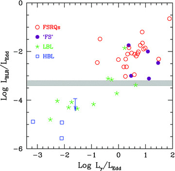
Luminosity of the BLR (in units of the Eddington one for sources with at least one broad line in their spectrum and with an estimate of the black hole mass) as a function of the γ-ray luminosity in units of the Eddington one. Empty (red) circles: FSRQs studied in G10 with estimates of the black hole mass and broad emission line luminosity; full (violet) circles: ‘FS’ sources (i.e. BL Lacs reclassified as FSRQs in this paper); (green) stars: LBLs; empty (blue) squares and upper limit: HBLs. The three data points for HBLs (Mkn 421, Mkn 510 and 2005−489) do not belong to the sample studied in this paper (i.e. they have αγ < 1/2), but are included for comparison.
The luminosity of the BLR in Eddington units for the γ-ray FSRQs studied in G10, for which there is an estimate of the black hole mass M. The specific value used for log M is indicated in square brackets in the last column. a: the SDSS associates the Mg ii line with the A iii+ C iii line, so the SDSS redshift is wrong. References: Be02: Bechtold et al. (2002); Ce97: Celotti et al. (1997); Li06: Liu et al. (2006); Os94: Osmer, Porter & Green (1994); Pi05: Pian et al. (2005); SDSS: Schneider et al. (2010), Shen et al. (2010) (https://www.cfa.harvard.edu/~yshen/BH_mass/dr7.htm); St93: Stickel et al. (1993).
| Name | z | Line | Ref | LBLR/LEdd |
| 0820+560 | 1.417 | Mg ii, C iii | SDSS | 7.7e-3 [9.3] |
| 0917+449 | 2.189 | C iv | SDSS | 8.7e-3 [9.8] |
| 0954+556 | 0.895 | Lyα | Be02 | 2.3e-3 [9.1] |
| 1013+054 | 1.714 | C iv | SDSS | 1.1e-3 [9.5] |
| 1030+61 | 1.401 | Mg ii | SDSS | 9.5e-4 [9.5] |
| 1055+01 | 0.89 | Mg iia | SDSS | 4.7e-3 [9.0] |
| 1144−379 | 1.048 | Mg ii | St93 | 9.7e-3 [8.5] |
| 1156+295 | 0.729 | Mg ii | SDSS, Pi05 | 7.8e-3 [8.7] |
| 1226+023 | 0.158 | Lyα, C iv | Pi05 | 3.3e-2 [8.9] |
| 1253−055 | 0.536 | Lyα, C iv | Pi05 | 2.3e-3 [8.9] |
| 1308+32 | 0.996 | Mg ii | SDSS | 8.1e-3 [8.9] |
| 1502+106 | 1.839 | C iv | SDSS | 8.2e-3 [9.5] |
| 1510−089 | 0.36 | Lyα, Mg ii | Ce97 | 4.9e-3 [8.6] |
| 1633+382 | 1.813 | Mg ii | St93 | 1.4e-2 [9.5] |
| 2141+175 | 0.211 | C iv | Os94, Li06 | 3.5e-3 [8.6] |
| 2227−088 | 1.559 | C iv | SDSS | 2.2e-2 [9.2] |
| 2230+114 | 1.037 | Lyα, C iv | Pi05 | 6.4e-2 [8.7] |
| 2251+158 | 0.859 | Lyα, C iv | Pi05 | 2.3e-1 [8.7] |
A clear trend is visible: objects with stronger emission lines are more luminous in the γ-ray band (normalizing both luminosities to the Eddington one). In this figure we have drawn a dividing line at LBLR/LEdd = 5 × 10⁻⁴, which separates ‘pure FSRQs’ and ‘FSs’ from the rest. The considered sources are still limited in number, but this division is in agreement with the idea that the blazars’ divide occurs for a change in the accretion regime. If we consider a disc luminosity roughly 10 times greater than LBLR, the separation from pure FSRQs to BL Lacs occurs at Ld∼ 5 × 10⁻³LEdd, approximately where the disc goes from a radiatively efficient to inefficient regime. This is in remarkable good agreement with what we suggested earlier (see GMT09 for Fermi blazars and Ghisellini & Celotti 2001 for FRI and FRII radio-galaxies).
BL Lac objects that we have reclassified as ‘FS’ indeed occupy the same region of FSRQs, confirming that the EW-based classification scheme sometimes hides the real nature of the source. ‘LBLs’ are intermediate sources, where the line luminosity (in Eddington units) decreases (but it does not disappear) as well as the γ-ray luminosity. ‘HBLs’ are at the extreme of the distribution, with very weak lines and weak Lγ. Consider furthermore that Fig. 3 shows only the sources with measured broad lines (there is only one exception, 1204−071, for which we have found an upper limit), and therefore we should not give too much weight to the apparent correlation between LBLR/LEdd and Lγ/LEdd. Consider also that luminosity variations exceeding even two orders of magnitude are not uncommon for these objects. Bearing these caveats in mind, we nevertheless believe that this figure indeed suggests that the sequence HBL → IBL (hopefully, no IBL is included, yet) → LBL → FSRQ can be explained as a sequence of strength of the broad lines.
The location of the points seems to suggest a continuity of LBLR/LEdd values, rather than a bimodal distribution, but the number of sources is really too small for a strong claim. We then leave this issue to future studies: these will give some insight on the properties of the ionizing flux: is it changing dramatically when the disc emits less than a few thousandths of the Eddington luminosity, or smoothly?
An important caveat is in order: we considered only the sources of known redshift, and as discussed in Section 2 there are many sources classified as BL Lacs in the 1LAC sample of unknown redshift. In order to discuss how these sources can affect the proposed classification scheme, consider the possibility that they all are at z = 0.5 or else at z = 2. In the first case, as Fig. 1 shows, they would have a low or moderate γ-ray luminosity. The fact that their spectrum is featureless implies that their emission lines are intrinsically weak, and if their black hole mass is similar to the other BL Lacs their LBLR/LEdd and Lγ/LEdd ratios locate these objects in the bottom-left region of Fig. 3, together with the shown sources.
Instead, if z∼ 2, these sources would have a γ-ray luminosity as large as the powerful FSRQs (the subset of these sources having αγ > 1.2 indeed occupies the same region occupied by FSRQs in Fig. 1). We have two possibilities.
They have powerful lines and an even more powerful continuum, swamping the emission lines. In this case, and for average black hole masses, their LBLR/LEdd is large, as it is Lγ/LEdd. They would then occupy the top-right part of Fig. 3, together with the other FSRQs. They would be sources similar to 0208−512, but with an even stronger continuum.
They have intrinsically weak lines, and average black hole masses. In this case LBLR/LEdd would be small, but Lγ/LEdd is large. They would then occupy the bottom-right part of Fig. 3, now devoid of sources. In this case there would be no correlation between LBLR/LEdd and Lγ/LEdd. These sources would have a powerful non-thermal emission, possibly extremely beamed (suggesting a very powerful jet), even if their accretion disc is weak.
We conclude that the new classification scheme we are proposing is not affected by the possible redshift values of the BL Lacs with unknown z. On the contrary, our physically based scheme could strengthen possible problems concerning the blazar sequence. In fact, in the latter mentioned case (i.e. z∼ 2 for the sources of unknown z) we could demonstrate the existence of very powerful sources that are classified as BL Lacs not only according to the ‘old’ definition (based on the EW), but also according to the one we are proposing.
The suggested new classification scheme can have important consequences and ramifications, which we discuss below.
6 DISCUSSION
The most important result of this study is the suggestion of a new classification criterion distinguishing BL Lac objects from FSRQs, based on the luminosity of the broad emission lines measured in Eddington units. The critical value we propose is around LBLR/LEdd∼ 5 × 10⁻⁴. We base this suggestion on the measurements of the emission line luminosities, on the estimates of the black hole mass and on the conversion of the luminosity of a few lines (often, only one line) into the luminosity of the ensemble of the broad emission lines. We find that the LBLR/LEdd ratio is proportional (with some scatter) to the γ-ray luminosity measured in Eddington units. If we furthermore divide the blazars into sub-categories according to the properties of their SED, then again we find a trend: low values of the LBLR/LEdd ratio correspond to low-power, high-energy emitting (i.e. ‘blue’) BL Lacs. Vice versa, high values of LBLR/LEdd correspond to powerful ‘red’ FSRQs. This is in total agreement with the blazar sequence, and also with the blazars’ divide we have proposed earlier.
We would like to stress that the distinction between FSRQs and BL Lacs we are proposing here does not imply a dichotomy. This could be present if the entire accretion disc suddenly changes regime below and above a given threshold in  , but more likely there should be a gradual change (namely, some parts of the accretion discs might be radiatively efficient and others not). Then the transition between BL Lacs and FSRQs might be gradual as well.
The first example of how this new classification might be useful concerns our starting sample of ‘intruder’ BL Lacs. Fig. 4 shows how the different types of intruder BL Lacs are located in the αγ−Lγ plane. Blazars re-classified as ‘FS’ all have large γ-ray luminosities (filled magenta circles) and fall in the same region of luminous FSRQs. LBLs span a large range of Lγ, but not the very high end, and can be thought as intermediate objects. HBLs are at significantly lower γ-ray luminosities. Of course one is left curious to see what happens for the remaining BL Lacs of this plot. To satisfy this curiosity we plan to systematically study them (Sbarrato et al., in preparation).

The other obvious advantage of our proposed classification is that it is physically based, and will help to construct cleaner samples of objects aiming to study possible different properties between BL Lacs and FSRQs, or, rather, between weak and strong line objects. For instance, this might help to clarify why some BL Lac objects, observed and imaged in the radio band, appear to be FR II radio-galaxies (see e.g. Kharb, Lister & Cooper 2010) contrary to the accepted scenario of the parent population of blazars, assigning FR I to BL Lacs and FR II to FSRQs. A particularly interesting issue that the new classification scheme will help to clarify is the evolution of blazars. Hints of no or slightly negative evolution of BL Lacs (or subcategories of them) and of positive evolution of FSRQs could be associated with the evolution of the accretion rate in cosmic time. It is possible that a better understanding may come from considering the entire blazar population as a whole, characterized by larger rates of accretion in the past (and therefore by a prevalence of FSRQs over BL Lacs) and a decreased rate of accretion now (with BL Lacs becoming more numerous). We believe that this idea, put forward, among others, by Maraschi & Rovetti (1994) and by Cavaliere & D’Elia (2002), is worth pursuing.
By linking the BLR luminosity to the underlying accretion luminosity we suggest that the different ‘look’ of blazars reflects primarily their accretion rate in units of the Eddington one. The  ratio controls the radiative efficiency of the accretion disc, and thus the absolute luminosity of the broad lines, and (through the BLR size–disc luminosity relation), their distance from the black hole. This in turn regulates the importance of the EC process for the formation of the high-energy bump of the SED. Powerful blazars do have powerful discs; luminous broad lines emitted at large distances. If jet dissipation occurs within the BLR, the EC process is dominant and the cooling severe, resulting in γ-ray-dominated sources. Weaker blazars have weak disc and weaker lines emitted closer to the black hole. Dissipation in the jet occurs outside the BLR; the main processes become synchrotron and SSC, resulting in more equally shared luminosity between the synchrotron and the SSC components.
The other strong evidence we have found in our earlier works (e.g. Celotti & Ghisellini 2008; G10; Ghisellini et al. 2010b) is that the total jet power Pjet is proportional to  , and indeed very close to
  independently of the accretion regime. The claim that
  depends somewhat on the assumption to have one proton per emitting electron. Although we do have limits to the possible amount of pairs (that cannot be energetically important; see Sikora & Madejski 2000, Celotti & Ghisellini 2008; Ghisellini & Tavecchio 2010) some uncertainty remains on the exact amount of pairs in jets. An almost model-independent lower limit on the jet power is the power spent by the jet to produce the non-thermal radiation, Pr. It is a lower limit because if Pr were comparable to the total jet power, Pjet, then the jet would strongly decelerate, and no superluminal motion would be seen. Assuming that Pr is proportional to Pjet implies a constant efficiency in converting part of the bulk relativistic motion into relativistic electrons and then radiation. Pr can be derived by equation (2) substituting, for Ui, the energy density of the radiation produced by the jet, evaluated in the comoving frame. The only free parameter entering in the estimate of Pr is the bulk Lorentz factor (Pr∝L/Γ2, where L is the bolometric luminosity of the jet, calculated assuming isotropy).
In Fig. 5, we show Pr as a function of the accretion luminosity Ld. It shows the blazars analysed in this paper together with the ones studied in G10 and Ghisellini et al. (2010b). For large values of Ld and Pr, the two quantities are proportional. Instead, below Ld∼ 1045 erg s−1, the data points and the shown upper limits are consistent with Pr∝L1/2d.
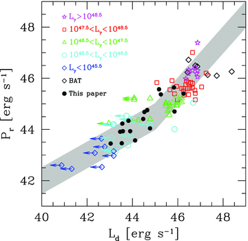
Power of the jet spent for the radiation Pr as a function of the accretion luminosity Ld. Black symbols are the estimates in this paper, BAT points (grey diamonds) come from the high-redshift blazars present in the 3-year all-sky survey of BAT (and studied in Ghisellini et al. 2010b), the other points and upper limits come from G10, and are divided according to their γ-ray luminosities, as labelled. The grey stripe indicates what is expected if  for all luminosities, while
  and
and  at low and high values of
  , respectively.
We interpret this behaviour (see also G10 and Ghisellini & Tavecchio 2008) as follows.
 . Instead, assume that
  , with η being constant only above a critical luminosity (in Eddington units), while below this critical value
  (Narayan, Garcia & McClintock 1997). This means that
  above some critical value Lc, and
  below. Assuming
  thus implies
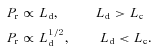
If the jet power is always proportional to  , its intrinsic properties should not change according to
  being smaller or greater than any critical value. In other words the jet properties should not depend on
  . Therefore, the jet power traces
  better than the accretion luminosity, which strongly depends upon
  . On the other hand, the ‘look’ of the jet (i.e. the produced non-thermal SED) is strongly influenced by
  because it is the latter ratio that rules the strength of the external radiation used as seed for the formation of the high-energy bump of the SED.
To reiterate, the jet power does depend on  linearly, but there is no dependence of the formation, collimation and acceleration mechanisms of the relativistic jet in blazars on
  . Relativistic jets are present for all values of
  .
.
7 SUMMARY AND CONCLUSIONS
In this work we have analysed a sample of blazars detected by Fermi/LAT that have been classified as BL Lac objects and that have an energy γ-ray spectral index αγ > 1.2. They therefore occupy a region, in the αγ−Lγ plane, preferentially occupied by FSRQs. Our intent was to investigate the properties of these objects, to see if they could be considered as intermediate objects between ‘pure’ BL Lacs and ‘pure’ FSRQs.
Doing so, we collected from the literature the broad emission line data for a sizeable number of these sources, as well as estimates of their black hole mass. At the same time, we model their SED with a one-zone leptonic model, to find out their intrinsic properties and especially to investigate why their γ-ray spectrum is rather steep. Our main results are the following.
From the model fitting, we explain the relatively steep αγ of these blazars as due to a relatively severe cooling of the electron population. The cooling is particularly severe in sources that have strong discs and emission lines, but also in the remaining sources it is fast enough to make the emitting electron distribution steep.
Some of the considered blazars, classified as BL Lacs, have broad emission lines as strong as in FSRQs, both in absolute terms and in Eddington units.
There is a trend associating the BLR luminosity in Eddington units with the γ-ray luminosity. Due to the paucity of points, we cannot claim that there is a strict correlation, yet the indication is that LBLR/LEdd, Lγ/LEdd and the type of the SED (i.e. LBL or HBL) are strongly linked.
From this evidence, we suggest a new classification scheme for dividing BL Lacs from FSRQs, based on the BLR luminosity in Eddington units: we propose to set the dividing value at LBLR/LEdd∼ 5 × 10⁻⁴.
Since the BLR is thought to intercept and reprocess about 10 per cent of the disc luminosity, the dividing value corresponds to a disc emitting at the ∼0.5 per cent of the Eddington limit. This is, approximately, also the value dividing the radiatively efficient from the radiatively inefficient accretion regimes.
This work, together with the previous studies we have done on Fermi (and EGRET) blazars, confirms that jets are powerful, and that they are born and launched for all values of the accretion rate (in Eddington units).
We thank the referee, P. Giommi, for useful criticism. This work was partly financially supported by an ASI (I/088/06/0) grant. This research made use of the NASA/IPAC Extragalactic Data base (NED) which is operated by the Jet Propulsion Laboratory, Caltech, under contract with NASA, and of the Swift public data made available by the HEASARC archive system.
REFERENCES
Appendix
APPENDIX A
[ SED of 0058+3311 and 0109+22. Darker points (red in the electronic version) refer to the Fermi/LAT and Swift (UVOT and XRT) observations. The lines are the result of the modelling. We label the synchrotron component (green solid line), the disc, torus and X-ray corona emission (dotted black), the SSC flux (grey long dashed) and EC flux (grey dot–dashed). The thick (blue) line is the sum of all components. ] [ SED of PKS 0208−512, PKS 0235+164, PKS 0426−380 and PKS 0521−365. Symbols and lines as in Fig. A1. ] [ SED of PKS 0537−441, PMN 0558−3839, PKS 0754+100 and PKS 0808+019. Symbols and lines are as in Fig. A1. ] [ SED of PKS 0829+046, 0851+202 (= OJ 287), 0907+3341 (= TON 1015) and 0954+658. Symbols and lines are as in Fig. A1. ] [ SED of 1012+0630, 1026−1748, PKS 1057−79 and B2 1147+24. Symbols and lines are as in Fig. A1. ] [ SED of 1204−071, B2 1338+40, PKS 1519−273 and 1557+565. Symbols and lines are as in Fig. A1. ] [ SED of PKS 1749+096, S5 1803+78, 1897+698 (= 3C 371) and S5 2007+77. Symbols and lines are as in Fig. A1. ] [ SED of 2200+420 (= BL Lac), B2 2214+24, PKS 2240−260 and 2340+8015. Symbols and lines are as in Fig. A1. ]


